Absolute quantitation of intracellular metabolite concentrations by an isotope ratio-based approach

Abstract

This protocol provides a method for quantitating the intracellular concentrations of endogenous metabolites in cultured cells. The cells are grown in stable isotope-labeled media to near-complete isotopic enrichment and then extracted in organic solvent containing unlabeled internal standards in known concentrations. The ratio of endogenous metabolite to internal standard in the extract is determined using mass spectrometry (MS). The product of this ratio and the unlabeled standard amount equals the amount of endogenous metabolite present in the cells. The cellular concentration of the metabolite can then be calculated on the basis of intracellular volume of the extracted cells. The protocol is exemplified using Escherichia coli and primary human fibroblasts fed uniformly with ¹³C-labeled carbon sources, with detection of ¹³C-assimilation by liquid chromatography–tandem MS. It enables absolute quantitation of several dozen metabolites over ~1 week of work.

INTRODUCTION

This protocol describes methodology for quantitating the concentrations of endogenous metabolites in cultured cells using MS, with the example described herein using liquid chromatography (LC)–tandem MS on a triple quadrupole mass spectrometer. Implementation of the protocol involves growing cells in a medium containing nutrients labeled with stable isotopes and then quenching metabolism and extracting metabolites in a solution spiked with unlabeled standards. Concentrations of metabolites in the cells are then calculated using the ratio of the labeled extracted metabolite to the unlabeled internal standard (see Fig. 1). This method has been used to investigate metabolites including glycolytic and tricarboxylic acid cycle intermediates, amino acids, nucleotides and folates from cells including E. coli, Salmonella enterica, yeast and human fibroblasts^1-6 (see also B.D.B. and J.D.R., unpublished data).

Figure 1.

Overview of workflow, illustrated for the case of nonadherent cells such as E. coli.

Cell culture, metabolism quenching and metabolite extraction

Many metabolites turn over very rapidly; thus, correctly measuring intracellular metabolite concentrations requires the ability to sample cells quickly. Otherwise, the measured levels will reflect the metabolic state induced by the handling steps leading up to quenching of metabolism, rather than normal cellular physiology. For adherent cells such as human fibroblasts, metabolism can be quenched with minimal perturbation of the culture simply via quick aspiration of medium and addition of cold organic solvent. The solvent addition stops metabolism (initially due to the temperature drop and subsequently by denaturing enzymes) and simultaneously initiates the extraction process by disrupting the cell membrane.

For nonadherent cells, such as E. coli or Saccharomyces cerevisiae, filter culture⁷ allows similarly rapid and nondisruptive metabolic quenching. In this method, cells are grown on a membrane filter sitting on top of an agarose plate loaded with media (Fig. 1). The cells are fed by nutrient diffusion from the underlying media up through the filter. For a given medium composition, the growth rate of the cells is comparable with those grown in standard batch culture³. In addition, the cells show comparable responses to nutrient deprivation^7,8. To quench metabolism and extract the intracellular metabolites, the membrane is simply moved from the agarose plate to a dish containing cold organic solvent. The move from plate to extraction solution can be done in ~1 s, during which there is little perturbation, as there are still extracellular nutrients contained in the liquid absorbed in the filter. Nevertheless, the cells are efficiently separated from the vast majority of their surrounding media without the delays and disruptions associated with filtering or pelleting a liquid culture.

Alternatives to filter culture include growing cells in standard liquid culture and separating them from their surrounding media by filtration or centrifugation. These approaches are generally acceptable for metabolites that turn over less rapidly. For example, we find that fast filtration (time scale approximately 5–10 s) gives adequate results for metabolites in steady-state cultures of yeast, but not for high flux metabolites like ATP or glutamine in E. coli. Other alternative approaches are described elsewhere^9,10. Approaches that involve washing of cells (e.g., with water or PBS) before quenching metabolism, despite facilitating subsequent analytical steps, generally result in unacceptable alterations of cellular metabolite composition and should be avoided^9,11.

A spectrum of solvent mixtures for metabolism quenching and metabolite extraction have been tested^1,12,13, and one may select an appropriate extraction solvent mix according to experimental needs. For extraction of filter cultures, we recommend a ratio of 40:40:20 acetonitrile/methanol/water in general, and this system with the addition of formic acid to a final concentration of 0.1 M for studies involving nucleotide triphosphates in E. coli. This recommendation is based on experiments showing that, for E. coli, there is a marked decrease in nucleotide triphosphate extraction (and increased conversion to less phosphorylated species) unless both acetonitrile and formic acid are added to the extraction mixture^1,14. Methanol extraction is recommended for extracting amino acids in E. coli (100% methanol for the first extraction and 80:20 methanol/water for the subsequent two extractions) and for extracting human fibroblasts (80:20 methanol/water for all three extractions). Extraction using these methods captures a mixture of free and (perhaps with lesser efficiency) macromolecule-bound intracellular metabolites. Accordingly, the present method is insufficient to differentiate free from bound metabolite pools.

Chromatography–MS

Once an extract is obtained, it can be analyzed using a wide variety of chromatography-MS procedures. For example, separation may be achieved by gas chromatography¹⁵, capillary electrophoresis¹⁶ or LC¹⁷, including variants of LC such as capillary monolithic chromatography^18-20 and ultra performance LC^21-24. In conjunction with capillary electrophoresis or LC, ionization may be achieved using electrospray ionization (ESI), atmospheric pressure chemical ionization or atmospheric pressure photoionization²⁵. We typically use LC coupled to ESI. An advantage of LC is its applicability to a broad diversity of analytes without the need for derivatization. A key advantage of ESI is its efficiency in converting charged compounds into gas phase ions. An important limitation of ESI is that it is a competitive process. Thus, an abundant ion can suppress the signals of less prevalent components (‘ion suppression’). Accordingly, the quality of LC separation is critical to the sensitivity of MS detection. Ion suppression can also lead to quantitative artifacts, as the signal of a compound in a complex mixture will be less than the signal of the same concentration of a pure standard. Such quantitative artifacts are corrected for by mass ratio-based analysis of the type described here, as both the labeled and unlabeled forms of the compound will be subject to quantitatively identical ion suppression.

There are a number of mass spectrometer options for analysis of the gas phase ions produced by LC-ESI or other chromatography–ionization approaches. These include quadrupole (most useful when arranged in series in a triple quadrupole instrument), ion trap, time-of-flight (TOF), Fourier transform ion cyclotron resonance and Orbitrap²⁶. Different types of analyzer can also be combined to form a hybrid mass spectrometer, such as a quadrupole-TOF instrument. Any of these mass spectrometer types can in concept be used to conduct the experiments described herein, with triple quadrupole MS the approach used by us to date and TOF representing an economical alternative.

For the present purposes, a triple quadrupole instrument is run in multiple reaction monitoring (MRM) mode. Instrumentally, three quadrupoles are arranged in series. The first selects a parent ion m/z of interest, the second fragments the parent ion and the third isolates a product ion m/z predetermined on the basis of preliminary experiments using purified standard of the metabolite of interest. To analyze multiple metabolites and isotope-labeling states, this process is repeated in a cyclic manner, with a dwell time of ~50 ms for each compound. The MRM approach benefits from excellent sensitivity and broad linear dynamic range. Its main disadvantages are the need to prespecify each compound of interest and a limit to the number of metabolites/labeling states that can be reliably analyzed in a given chromatography interval. It is most readily used to measure only fully labeled and fully unlabeled compounds. Partially labeled forms can also be measured, but it takes a longer scan time, as different locations of isotope label may result in different product ion masses (i.e., the labeled carbon may or may not end up in the product ion, depending on its position in the parent). An ion-trap instrument can be used to conduct MRM, but with less sensitivity and dynamic range.

TOF involves a conceptually simpler MS approach: every ~1 s, a readout is taken of whatever ions are present. Selectivity, which is obtained in the MRM approach via the MS/MS, is obtained in TOF by mass accuracy (i.e., separation of compounds of the same nominal m/z by their exact mass). Full-scan methods like TOF enable monitoring of all isotopic forms of a metabolite. The main disadvantages of TOF relative to MRM are somewhat reduced sensitivity and dynamic range. In addition, information about the location of the isotope label within a partially labeled species is not available. Orbitrap and Fourier transform ion cyclotron resonance and provide similar data to TOF but are currently more expensive.

Irrespective of the LC-MS approach that is used, it is ultimately necessary to quantify the intensities of mass-specific chromatographic peaks. Software for peak intensity quantitation is included in most commercial LC-MS packages and generally allows quantitation on the basis of peak area or peak height at the user’s discretion. Both give equivalent results for Gaussian peaks. Typically, we quantify on the basis of peak height, as it is somewhat less sensitive than peak area to baseline fluctuations. Alternative metrics, such as the mean height of the top few points in an MRM peak, are also equally valid and may offer subtle improvements in reproducibility.

Workflow and data interpretation

A detailed flowchart of the experimental workflow is illustrated in Figure 2. Cells are grown in isotopically labeled medium to the desired density, at which point the cells are quickly transferred to cold organic solvent spiked with standards. The presence of the internal standards in the quenching/extraction solution is critical, as the internal standards experience similar conditions to the cellular metabolites, especially to the free intracellular metabolites, thereby controlling for degradation and adsorption during the extraction process. Standards are spiked into the extraction solution only during the first step, with unspiked solvent used for subsequent steps. The isotopic standards in the resulting final extract control for ion suppression and other sources of LC-MS variability. Best results are obtained if standard concentrations are close to the concentration of the metabolite in the extract. Intracellular concentrations are then determined by the ratio of the peak sizes of the cellular metabolite to the standard, as originally described by J.J. Heijnen⁶ and colleagues.

Figure 2.

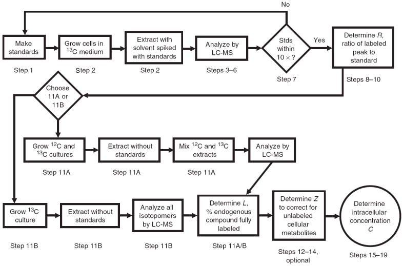
Flowchart of protocol steps.

If labeling of the cellular compound of interest is substantially complete, then analysis is straightforward. Figure 3 shows a hypothetical example involving a 4-carbon compound, such as malate or aspartate, and labeling with uniformly ¹³C-glucose. For simplicity, the example assumes that the quantity of spiked unlabeled compound (blue) exactly equals that of endogenous compound (yellow). Figure 3a exemplifies the ideal case of complete labeling. The fully labeled and fully unlabeled peaks are almost equal, except that a small amount (~4%) of the spiked unlabeled compound has a single ¹³C atom due to the natural abundance of ¹³C. The ratio R, defined as the intensity of the fully labeled peak divided by the fully unlabeled peak (corrected for losses of the fully unlabeled form due to the natural abundance of ¹³C), is 1 (see Step 8).

Figure 3.

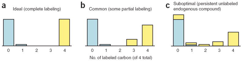
Schematic of potential mass spectrometry peak intensities obtained via Steps 2–6 for a 4 carbon compound after ¹³C labeling. Blue indicates signal arising from the spiked unlabeled internal standard. Yellow indicates signal arising from endogenous cellular compound after feeding the cells with uniformly ¹³C-labeled carbon source. The total amounts of spiked and endogenous compounds are shown as being equal for simplicity. (a) Case A involves complete labeling of the cellular compound, in which L = 1, Z = 0 and Steps 11–16 could be omitted. (b) Case B involves some of the cellular compounds being only partially labeled. In this case, L < 1 and Steps 11–13 provide an important quantitative correction; however, Z = 0 and Steps 14–16 could be omitted. (c) Case C involves some of the cellular compound remaining fully unlabeled. In this case, Z > 0 and all steps are required.

We find that extended growth in uniformly ¹³C-labeled glucose will lead to complete labeling of many metabolites in E. coli or yeast (as shown in Fig. 3a)^4,5,17. For many other metabolites, however, partially labeled forms are also found, primarily due to assimilation of unlabeled carbonate (e.g., by the reactions generating oxaloacetate from pyruvate or phosphoenolpyruvate)⁵. This results in labeling patterns like the one shown schematically in Figure 3b. In this case, even though the spiked standard (blue) and endogenous compound (yellow) are equally abundant, the ratio R is less than 1. This necessitates a correction factor (termed L) reflecting that fraction of the endogenous compound in the fully labeled form. If data on partially labeled forms are available, this factor can be determined as the fraction of the labeled form that is fully labeled (see Step 11A). If MRMs that provide information solely on the fully labeled and fully unlabeled forms are being used, then L can be calculated by comparing the peak of the fully labeled form (in cells grown on labeled nutrient) with the fully unlabeled form (in cells grown on unlabeled nutrient) (see Step 11B).

For mammalian cells, calculations are further complicated by persistence of fully unlabeled endogenous forms of certain compounds. For example, feeding with both U-¹³C-glucose and U-¹³C-glutamine over ~5 d and 2+ doublings leads to incorporation of ¹³C into most metabolites in cultured mammalian fibroblasts, but a nontrivial amount of certain metabolites persist in the fully unlabeled form. This results in labeling patterns like the one shown schematically in Figure 3c, in which the peak of the spiked, unlabeled compound is ‘contaminated’ with unlabeled endogenous compound. The extent of contamination can be estimated by measuring the relative peak intensities of the fully unlabeled and fully labeled forms in cells fed with labeled nutrient and extracted in the absence of any spiked standard. We term this ratio Z. The product R × Z represents the fraction of the unlabeled signal observed in the experiment for determining R, which arose from unlabeled endogenous compound (i.e., the fraction of the peak with zero labeled carbons in Fig. 3 that is ‘yellow’). A large value of R × Z potentially leads to large error in the calculation of the metabolite concentration, and as such, we suggest repeating any measurement for which R × Z > 0.25. If Z is small, this correction will generally not be necessary, as the error caused by this small amount of unlabeled metabolite will not be significant when compared with the overall error. For example, in Figure 3a and b, and in general in experiments with microbes, Z is ~0.

All calculations in the procedure are done using geometric means, as is appropriate when dealing with ratios. In the protocol, error is calculated as the variance of the logarithm until the final determination of a concentration confidence interval (which is nonsymmetrical, being larger in the upward than downward direction). A step-by-step guide for calculating the errors of the determined concentrations is provided. Typically, we recommend conducting ~4 replicates of each measurement, which generally results in 95% confidence intervals on metabolite concentrations spanning an ~2- to 4-fold range. Tighter confidence intervals are generally found for stable, abundant compounds and broader ranges for less stable or low-abundance compounds. For compounds present in cells in concentrations <100 μM, quantitation is often difficult, unless the compound ionizes well. Similarly, quantitation of compounds with intrinsic decay half-times of <6 h is difficult, unless suitable preservatives can be identified (e.g., ascorbate for folates²⁷).

In the initial application of this protocol, it may be useful to begin by replicating literature results (e.g., if working with E. coli, regarding glutamate, glutamine and adenosine nucleotide concentrations^1,8). Once the protocol is up and running, it can be a useful tool for addressing basic questions such as the following: which are the most abundant metabolite species in cells? Along specific pathways? How do intracellular substrate concentrations compare to the Michaelis constants (K_m) of enzymes; that is, which enzymes are saturated or not saturated with substrates in live cells? Answers to these questions are essential for the quantitative analysis of metabolism and its regulation, and ultimately for the rational manipulation of metabolism to meet medical and bioengineering objectives.

MATERIALS

REAGENTS

• HPLC-grade water (EMD, cat. no. WX0004-1)

• HPLC-grade acetonitrile (OmniSolv, cat. no. AX0142) ! CAUTION Wear gloves and safety glasses when handling acetonitrile.

• HPLC-grade methanol (OmniSolv, cat. no. Mx0488P-1) ! CAUTION Wear gloves and safety glasses when handling methanol.

• Ammonium hydroxide, 29%, for HPLC buffer (Fisher Scientific, cat. no. A669) ! CAUTION Wear gloves and safety glasses when handling ammonium hydroxide.

• Ammonium acetate for HPLC buffer (Mallinckrodt Chemicals, cat. no. 3272-02) ! CAUTION Wear gloves and safety glasses when handling ammonium hydroxide.

• Formic acid, 88% (optional), depending upon extraction solution (Fisher Scientific, cat. no. A118P-500) ! CAUTION Wear gloves and safety glasses when handling formic acid.

• Ammonium bicarbonate (optional) depending upon extraction solution; use to neutralize extract if initially extracting in presence of formic acid (Fluka, cat. no. 09830)

• Standards of any metabolites you wish to quantify

• U-¹³C glucose (Cambridge Isotope Laboratories, cat. no. CLM-1396)

• U-¹³C glutamine for mammalian cell culture (Cambridge Isotope Laboratories, cat. no. CLM-1822)

• Minimal medium components for microbial culture:

  • Potassium phosphate, monobasic (Sigma-Aldrich, cat. no. P0662)
  • Potassium phosphate, dibasic (Sigma-Aldrich, cat. no. P8281)
  • Potassium sulfate (Sigma-Aldrich, cat. no. P9458)
  • Magnesium sulfate heptahydrate (Sigma-Aldrich, cat. no. M1880)
  • Ammonium chloride (Fisher Scientific, cat. no. A661)
  • ¹²C-glucose (Fisher Scientific, cat. no. D16)

• Ultrapure agarose (Invitrogen, cat. no. 15510-027) (for microbial filter culture)

• DMEM without glucose or glutamine, for mammalian cell culture (Mediatech Inc., cat. no. 10-017)

• HEPES buffer, for mammalian cell culture (Acros Organics, cat. no. AC17257-0010)

• 100 mm × 15 mm sterile Petri dishes (Fisher Scientific, cat. no. 08-757-12) for making agarose plates for filter cultures; for culturing of adherent mammalian cells, select instead the Petri dish surface chemistry most appropriate for growth of your specific cell line

• 15-ml sterile polypropylene conical tubes, for growing 5 ml of overnight cultures, for microbes (BD Falcon, cat. no. 14-959-70C)

• Sterilized flask for growing liquid cultures of the microbes, in preparation for subsequent filter culture

• 82-mm nylon membrane filters for microbial filter cultures (GE Water & Process Technologies, cat. no. N00HY08250)

• 1.7-ml microcentrifuge tubes (Bioexpress, cat. no. C-3269-1)

• Dry ice if using methanol extraction

• Cell scraper for adherent cells (Fisher Scientific, cat. no. 08-773-1)

EQUIPMENT

• Pipette filler/dispener (a motorized one is recommended) and 5-ml pipettes

• Vortex mixer (Fisher Scientific, cat. no. 02-215-365)

• HPLC-ESI-MS/MS (see EQUIPMENT SETUP)

• HPLC vials and caps (Fisher Scientific, cat. no. 033778D)

• Tweezers for manipulating the membrane filters, for filter cultures (Fisher Scientific, cat. no. 02-215-365)

• Shaker table, for growing liquid cultures; this is typically placed in a 37 °C warm room or incubator (for microbial cultures)

• Spectrophotometer (Thermo Electron Corp, Genesys 10 uv) used at 650 nm for measuring optical density

• Plastic cuvettes (Fisher Scientific, cat. no. 14-955-127) (for microbial cultures)

• Microcentrifuge, for pelleting cell debris after extraction (Eppendorf, cat. no. 5415D). If a microcentrifuge is not available, a normal centrifuge may be used

• −20 °C freezer (when using 40:40:20 acetonitrile/methanol/water extraction mixture)

• Metal pan, and icepacks to fill, precooled to −20 °C (when using 40:40:20 acetonitrile/methanol/water extraction mixture)

• N-evap evaporation system (Organomation Associates Inc., cat. no. 11155-0). Optional, use only if sample concentration is required to get adequate signal

REAGENT SETUP

Cells

Before initiation of an experiment, cells should be handled as per typical laboratory protocols tailored to the cell type of interest. To initiate this protocol, a starter culture is required for microbes and 10⁶–10⁷ cells in culture for mammalian cells.

Washed agarose for microbial filter cultures

Wash the Ultrapure agarose three times with HPLC-grade water to remove trace impurities. For 30 g agarose, use 1 liter of water for each wash. For each wash, stir the agarose–water mixture for 10 min and allow to settle for ~1 h. Aspirate the water with care to avoid loss of agarose. The resulting washed agarose can be used to make minimal media plates with 1.5% agarose.

Minimal liquid medium with and without isotopically labeled nutrient (for microbial cultures)

Combine sterile salts, U-¹³C glucose, water and agarose according to your media recipe. (The exact composition of the complete minimal media we use is as follows: KH₂PO₄ 4.7 g liter⁻¹, K₂HPO₄ 13.5 g liter⁻¹, K₂SO₄ 1 g liter⁻¹, MgSO₄ · 7 H₂O 0.1 g liter⁻¹, NH₄Cl 10 mM, glucose 0.4%; make the media with U-¹³C-glucose and separately with unlabeled glucose.)

Minimal medium plates with and without isotopically labeled nutrient (for filter cultures)

Combine minimal liquid medium (with U-¹³C-labeled glucose when appropriate) with 1.5% agarose. Autoclave and pour into the sterile Petri dishes to make plates. Use 15–25 ml of agarose-medium mixture per 10-cm plate.

Liquid DMEM with and without isotopically labeled nutrient (for mammalian cell cultures)

Add U-¹³C-labeled glucose and glutamine (and, separately, unlabeled glucose and glutamine) to the DMEM media without glucose and glutamine, to obtain complete labeled and unlabeled DMEM media. Final glucose and glutamine concentrations should be 4.5 g liter⁻¹ and 584 mg liter⁻¹, respectively.

Extraction solutions

Different groups of metabolites are extracted with different efficiency depending upon the extraction solution mixture¹. Choice of extraction solution should be made according to which metabolites are of the greatest interest. Among the solution systems that we have tested for extracting filter cultures, 40:40:20 acetonitrile/methanol/water solvent system works the best for extracting filter cultures in general; addition of formic acid to a final concentration of 0.1 M provides additional protection of nucleotide triphosphates against degradation¹. Methanol (100% methanol on dry ice for the first round, 80:20 methanol/water at 4 °C for the two subsequent rounds) extracts amino acids efficiently while extracting fewer other components than acetonitrile/methanol/water; it is accordingly preferred for studies focused solely on amino acids. For extracting human fibroblasts, we have obtained adequate results with 80:20 methanol/water for all three extractions. Pending more definitive studies, we recommend this solvent mixture for them.

Stock solutions of standards

Standards of each metabolite for which quantification is desired should be made to a high concentration (typically 0.1–1.0 mg ml⁻¹) in the solvent to be used for extraction. If you are using an acidic extraction solution, omit the use of the acid while making up the standard solutions. Stock solutions should be stored at −80 °C after preparation.

HPLC mobile phase

Solvent A: 20 mM ammonium acetate + 20 mM ammonium hydroxide in 95:5 water/acetonitrile, pH 9.45; Solvent B: acetonitrile. Note that this is our mobile phase of choice when working with aminopropyl column in hydrophilic interaction chromatography mode¹⁷; there are many other chromatography choices available^28-30. Many of these have important advantages relative to the aminopropyl approach for certain classes of compounds.

EQUIPMENT SETUP

Glass vacuum filtration apparatus

The components are listed below (for filter cultures), as shown in Figure 4:

Figure 4.

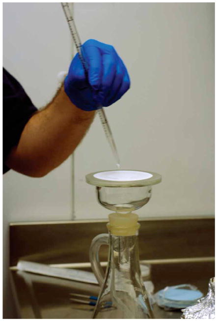
Creating filter culture from batch culture (Step 2A(vi)). Batch culture is slowly and evenly dripped onto a filter membrane, which sits on a sintered support base residing on top of a vacuum flask.

• Microanalysis vacuum filter holders, stopper, perforated, No. 8 (Fisher Scientific Ltd, cat. no. 09-753-32A)

• Microanalysis vacuum filter holders, sintered support base, diameter: 90 mm (Fisher Scientific Ltd, cat. no. 09-753-27B)

• Vacuum filtering flask, 1 liter

HPLC system

Hydrophilic interaction chromatography is performed on a 2-mm inner diameter column packed with 5-μm aminopropyl resin to 250 mm in length, using an LC-10A HPLC system (Shimadzu). The column is maintained at 15 °C with a solvent flow rate of 0.15 ml min⁻¹, and the gradients are as follows: t = 0, 85% B; t = 15 min, 0% B; t = 28 min, 0% B; t = 30 min, 85% B; t = 40 min, 85% B. Other chromatographic approaches and/or HPLC systems can be used depending on their availability and the metabolites of interest.

Mass spectrometer

A Finnigan TSQ Quantum Ultra triple quadrupole mass spectrometer (Thermo Electron Corporation) is run in MRM mode and coupled to the HPLC via ESI. ESI spray voltage is 3,200 V in positive ionization mode and 3,000 V in negative ionization mode. Nitrogen is used as sheath gas at 30 psi and as the auxiliary gas at 10 psi, and argon as the collision gas at 1.5 mTorr, with a capillary temperature of 325 °C. The mass spectrometer and LC system with autosampler are shown in Figure 5.

Figure 5.

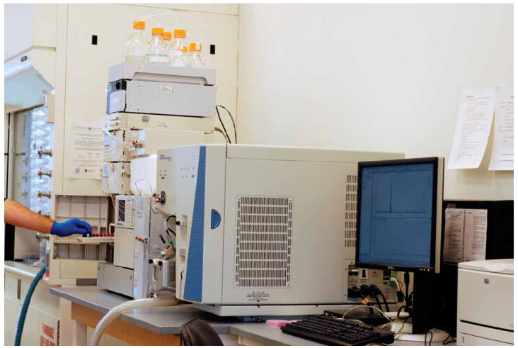
Triple quadrupole LC–MS/MS system.

MRM scans

Reactions should be optimized for metabolites of interest using standards before the quantification experiment. A list of reactions used in our experiments has been published previously¹⁷. Optimization of the product ion and collision energy for a given unlabeled metabolite is achieved by infusing purified compound standard into a triple quadrupole mass spectrometer. Collision energy should be identical for labeled and unlabeled forms. For ¹³C labeling, the parent ion mass should be increased by the number of carbon atoms in the metabolite, and the product ion mass by the number of carbon atoms in the product ion (product ion structures can be obtained from the literature for common metabolites, or otherwise estimated on the basis of common routes of fragmentation and confirmed experimentally by MS/MS of the labeled forms). For partially labeled forms, more than one product ion mass may be possible for each parent ion mass. The different product ion masses arise from labeling at different positions within the parent. As an example, consider the possibilities for a 4 carbon compound that gives a 3 carbon product ion (e.g., aspartate): with 0 × ¹³C in the parent, there cannot be ¹³C in the product ion; with 1 × ¹³C in the parent, there can be 0 or 1 × ¹³C in the product ion; with 2 × ¹³C in the parent, there can be 1 or 2 × ¹³C in the product ion; with 3 × ¹³C in the parent, there can be 2 or 3 × ¹³C in the product ion; with 4 × ¹³C, there must be 3 × ¹³C in the product ion.

PROCEDURE

1. Prepare a mixture of metabolite standards by dissolving the corresponding chemicals separately in the extraction solution of choice (see the INTRODUCTION and REAGENT SETUP). Mix appropriate amounts of the standard solutions together and dilute with the extraction solvent of choice. The final concentration of each metabolite standard in the extraction solution should be similar to the anticipated concentration of intracellular metabolite in the solution after extraction of the cells (i.e., the peak of the standard should approximate the intracellular metabolite peak within ~10-fold). In many cases, achieving this will require a preliminary experiment to estimate the appropriate standard amount. When no other information is available, we recommend a target concentration of 25 ng ml⁻¹ for each metabolite standard; however, required amounts may vary by orders of magnitude depending upon the metabolite. Store individual standard solutions at a cold temperature, with care to limit the duration of storage of less stable compounds after their dissolution (e.g., for ATP, we typically discard the standard solution after 7 d). To minimize errors caused by degradation of standards, use the standard mixture within 24 h of preparation and store at −20 °C or less. It is generally feasible to work with 10–20 different compounds at once. If studying a large number of compounds, try to group related compounds together (e.g., amino acids, nucleotides, etc.) and to avoid mixtures that contain metabolites that may chemically react (e.g., amines and aldehyde-containing metabolites).

2. Prepare isotope-labeled cell extracts. Option A is designed for nonadherent microbes and option B is designed for adherent mammalian cells.

   1. Grow, quench and extract U-¹³C-labeled non-adherent microbes

      1. Prepare agarose plates. You will need plates equal to the number of extracts you wish to generate (we recommend four) and two or three additional plates to determine optical density at 650 nm (OD₆₅₀) before extraction. Allow agarose plates to cool to room temperature (~25 °C).
      2. Inoculate your microbial strain into 5 ml of minimal medium with U-¹³C-glucose and grow overnight.
      3. Before use, warm all the plates to the temperature at which the cells are grown (i.e., 37 °C for E. coli) by placing them in a warm room or incubator.
      4. Add ~1 ml of the overnight culture to a flask containing 50 ml of fresh minimal medium with U-¹³C-glucose to OD₆₅₀ ~0.03 and allow to grow in batch to early exponential phase (OD₆₅₀ of ~0.1). Determine the total volume of batch culture according to the number of plates you will need for the experiment; 5 ml of the batch culture will be needed for each plate and ~5 ml extra for OD measurements, before creating the filter cultures. OD can be measured by pipetting 1 ml of your liquid culture into a spectrophotometer cuvette and measuring absorbance at 650 nm, using fresh media as blank.
      5. Assemble the vacuum filter support, stopper and vacuum filter flask as shown in Figure 4. Connect the side arm of the filter flask to a vacuum valve or pump (get the assembly ready before your batch culture reaches an OD₆₅₀ value of 0.1). If possible, place the whole assembly in a warm room to avoid temperature perturbation while preparing your filter cultures.
      6. Open the vacuum to a moderate level. Lay a membrane filter on the filter support with a pair of tweezers. As shown in Figure 4, pass 5 ml of your liquid culture (OD₆₅₀ ~0.1) through the membrane filter carefully using a pipette and dispenser. Slowly drip your culture in drops as evenly as possible onto the filter, leaving a small area near the edges uncovered. Remove the membrane filter from the filter support once the 5 ml of culture is loaded. Place it on an agarose plate with the cell side facing up, being careful to ensure that the filter makes good contact with the agarose over the entire cell-containing area. This step usually takes 30–60 s per filter.
      7. Repeat until loading all plates with the filter cultures has been completed.
         ▲CRITICAL STEP Be consistent when loading cells on to the filter to minimize variations between your filter cultures. Pay attention to the vacuum level, the speed at which you drip the liquid onto the filter and so on.
      8. Allow your filter cultures to grow to mid-log phase. Determine OD₆₅₀ by thoroughly washing a filter with 5 ml of water and measure the OD of the wash using the spectrophotometer. To wash the cells off the filter completely, one effective approach is to tilt the filter slightly and pipette the water onto the filter with mild pressure strong enough to produce a steady stream but not to cause a splash. E. coli typically take 2–2.5 h to grow to an OD₆₅₀ of 0.4 after completion of Step A(vi). We recommend checking OD₆₅₀ 2 h after preparing the filter cultures, then checking again at a later time point, if the target OD₆₅₀ has not yet been reached.
      9. Label a Petri dish for each filter culture to be extracted, add 2.5 ml of extraction solution (containing internal standards) to each dish and cool the dishes to the appropriate extraction temperature (−80 °C freezer or dry ice for methanol extraction; −20 °C freezer for 40:40:20 methanol/acetonitrile/water) for at least 10 min prior to filter culture extraction.
      10. After the filter cultures have been grown to the desired OD, peel each filter off the agarose plate with tweezers and immerse it in the extraction solution contained in a Petri dish, with the cell side down, as shown in Figure 6. Tilt the dish to ensure that the filter is completely covered by the extraction solution. Allow it to remain for 15 min at the extraction temperature (e.g., at −20 °C for 40:40:20 methanol/acetonitrile/water extraction). If working with a −80 °C extraction solution, do all work on dry ice, leaving the dish in contact with the dry ice as much as possible. If working with a −20 °C extraction solution, keeping the dishes on a surface precooled to −20 °C (such as a metal pan filled with ice packs) will help maintain the low temperature. Return dishes to the −20 °C freezer as soon as possible.
          ▲CRITICAL STEP Move the cells from the agarose plate to the cold organic solvent as quickly as possible to avoid metabolic perturbations.
      11. Rinse the filter with the extraction solution in the dish, as shown in Figure 7, and transfer the resulting solution, together with cell remnants suspended in it, into two microcentrifuge tubes. Add 1 ml of fresh extraction solution (without internal standards) to the dish and use it to re-rinse the filter. Add the resulting solution, together with any remaining cell remnants, to the 2.5 ml of initial cell extract in the microcentrifuge tubes.
      12. Centrifuge in a microcentrifuge at full speed (16,000g) at 4 °C for 5 min to pellet the insoluble materials. (Microcentrifuge and matching tubes are used here for easier pelleting of the cellular debris; they can be substituted with a regular tabletop centrifuge and use of a single larger tube, rather than two microcentrifuge tubes, if desired).
      13. Transfer the supernatant from the two microcentrifuge tubes into one clean conical tube and set aside at appropriate temperature (e.g., at −20 °C for 40:40:20 acetonitrile/methanol/water extraction).
      14. Resuspend the pellets in 100 μl (i.e., 50 μl per pellet) of extraction solution (without internal standards) and combine into one tube. Allow it to remain for 15 min at the appropriate temperature (e.g., −20 °C for 40:40:20 acetonitrile/methanol/ water extraction). If using 40:40:20 methanol/acetonitrile/water as extraction solution, little pellets will form here. Depending upon the size of the pellet, you may choose to skip either Steps 2A(xiv–xvii) or only Step 2A(xvii).
      15. Pellet in a microcentrifuge at full speed (16,000g) at 4 °C for 5 min.
      16. Mix the supernatant with the original supernatant from Step 2A(xiii).
      17. Repeat Steps 2A(xiv–xvi) to generate the complete cell extract of one filter culture.
      18. Neutralize the extract in each tube with 300 μl of 15% NH₄HCO₃ if using acidic acetonitrile/methanol/water extraction. Centrifuge at 16,000g at 4 °C one more time after neutralization to remove precipitates.
      19. Repeat Steps 2A(x–xviii) above for each filter culture.
   2. Grow, quench and extract U-¹³C-labeled adherent fibroblasts

      1. Prepare 24 ml of media with U-¹³C glucose and U-¹³C glutamine for each sample you plan to generate (we recommend N = 4). The medium should be buffered with HEPES to a final concentration of 10 mM to keep the pH relatively constant during media changes.
      2. Culture cells in a 10 cm Petri dish with 8 ml of labeled media for each sample. We recommend that this step be done over at least two cell doublings to get a high percentage of metabolites labeled.
         ■PAUSE POINT 2–7 d, depending upon cell culture growth rate.
      3. Twenty-four hours before extraction, aspirate the media in the Petri dishes and replace with 8 ml of fresh labeled media. The fresh media used in this step should be equilibrated in the incubator overnight before the media change.
      4. Repeat Step 2B(iii) 1 h before extraction.
      5. Aspirate the media completely and add 4 ml of the extraction solution (containing internal standards) prechilled to the appropriate temperature (−80 °C for methanol extraction). Let sit for 15 min at the extraction temperature (−80 °C for methanol extraction). Scrape the cells off the dish with a cell scraper. Transfer the cell suspension into a 15-ml conical tube. Centrifuge for 5 min at 2,000g and 4 °C to pellet the cellular debris. Transfer the supernatant into a new 15-ml tube and set aside.
      6. Resuspend the pellet in 500 μl of extraction solution (without internal standards) by vortexing and allow to remain at 4 °C for 15 min. Centrifuge for 5 min at 2,000g and combine the supernatant with the supernatant from Step 2B(v).
      7. Repeat Step 2B(vi) for a third round of extraction.
      8. Repeat Steps 2B(v–vii) for all remaining dishes.

3. (Optional) For each sample, evaporate the cell extract under N₂ gas flow (using an N-Evap system) until dry. Resuspend in 200 μl of 1:1 methanol/water solution. Be aware that, although this step will increase the metabolite concentration in the sample, it could also potentially cause increased ion suppression and loss of less stable metabolites. This step is generally unnecessary for microbial cell cultures, but it may be of value in some mammalian cultures.

4. Transfer the cell extract into HPLC vials and load the vials into the LC-MS autosampler.

5. Analyze the samples by LC-MS, using 10 μl injection volume (more if necessary; be aware that this may result in increased ion suppression), preprogrammed LC gradient and (for triple quadrupole mass spectrometry) preprogrammed MRM scan events.

   ■PAUSE POINT LC-MS runs can be done overnight.

6. For individual metabolites, quantify peaks of unlabeled and isotopically labeled forms using predefined MRM channels and appropriate program (or alternative MS-based approach).

7. Assess whether the magnitudes of the unlabeled standard and ¹³C-labeled cellular metabolite peaks are adequately similar. If peaks differ in size by more than roughly 10-fold, repeat Steps 1–6 using a new concentration of standard (S_new). The concentration to use is as follows:

   $$S_{\mathrm{new}}=S_{\mathrm{old}}\times \exp \left(\frac{1}{N}\sum _1^N\ln \left(\frac{P_{\mathrm{labeled}}}{P_{\mathrm{unlabeled}}}\right)\right)$$

   where P is the peak height of the corresponding form, S_old is the original concentration of the standard in the extraction solution used in Step 1 and N is the number of experimental replicates. If the magnitudes of the unlabeled and labeled peaks are adequately similar, proceed to Step 8.

8. For each sample, calculate the ratio of the labeled and unlabeled peaks, correcting for the decreased size of the unlabeled peak due to the naturally occurring heavy isotopes of carbon in the standards. The corrected ratio R is as follows:

   $$R_i=I\times \left(\frac{P_i^{\mathrm{labeled}}}{P_i^{\mathrm{unlabeled}}}\right)$$

   where P_i^labeled and P_i^unlabeled are the peak heights of the fully labeled and fully unlabeled forms, respectively, of the metabolite in the ith sample, and I = (0.9893)^{no. of carbons}. The value 0.9893 is the natural abundance of the carbon-12. The number of carbon atoms in the metabolite should be substituted appropriately.

9. Calculate the ratio of the labeled peak to the standard (R_avg) as follows:

   $$R_{\mathrm{avg}}=\exp \left(\frac{1}{N}\sum _{i=1}^N\ln R_i\right)$$

   where N is the number of replicates and R_i is as determined in Step 8.

10. Calculate the variance of R_avg in logarithmic space as follows:

    $${\sigma }_{\ln R}^2=\frac{1}{N-1}\sum _{i=1}^N{\left(\ln \frac{R_i}{R_{\mathrm{avg}}}\right)}^2$$

    where N is the number of replicate cultures studied and R_i and R_avg are calculated as described in Steps 8 and 9, respectively.

11. Determine the fraction of compound fully labeled (L, which potentially ranges from zero to one). This step is important in cases where incomplete labeling of the endogenous metabolites has occurred (as shown schematically in Fig. 3b and c). Common causes of this are the assimilation of unlabeled bicarbonate or incomplete turnover of endogenous metabolites or their precursors. Option A involves calculating L by quantifying both partially and fully labeled forms from labeled cellular extracts. Ideally, this requires examining peaks for all possible labeling patterns of the metabolite, although a reasonable approximation in many situations is to examine only the fully labeled forms and the forms that have unlabeled carbons from reactions known to incorporate carbonate into metabolites. Option B involves calculating L by comparing peaks from separate labeled and unlabeled cellular extracts. Option A is generally preferred when using TOF MS, but can be inconvenient when using triple quadrupole MS due to the need to include MRM scans for a large number of partially labeled forms. In such a case, option B provides an alternative.

    1. Determine the peak height of the fully labeled form, compared to all other forms

       1. If using a triple quadrupole mass spectrometer in MRM mode, create a mass spectrometry method that detects all carbon labeling patterns of the metabolites of interest (see MRM scans section under EQUIPMENT SETUP).
       2. Carry out Steps 2–6, growing cultures in ¹³C-labeled media, and extract using solvent without internal standards throughout. Typically, we recommend growing four cultures.
       3. For each sample, calculate L as follows:
          $$L_i=\frac{P_i^{\mathrm{labeled}}}{P_i^{\mathrm{tot}}}$$
          where P_i^labeled is the peak height of the fully labeled form of the metabolite, and P_i^tot is the sum of the peak heights of all forms of the metabolite.
    2. Compare ¹³C-labeled cultures to unlabeled cultures

       1. Carry out Step 2, but grow an equal number of cultures in unlabeled and ¹³C-labeled media throughout, and extract using solvent without internal standards throughout. Typically, we recommend growing four cultures in unlabeled and a separate four cultures in ¹³C-labeled media.
       2. Combine the extract from the ¹³C-labeled cultures to create one large pool of labeled extract.
       3. Combine each unlabeled filter extract from Step 11B(i) in a 1:1 ratio with the labeled pool created in Step 11B(ii), creating four separate samples for HPLC/MS analysis.
       4. Follow Steps 4–6.
       5. Calculate L as follows:
          $$L_i=I\times \left(\frac{P_i^{\mathrm{labeled}}}{P_i^{\mathrm{unlabeled}}}\right)$$
          where I is calculated as described in Step 8, and P_i^labeled and P_i^unlabeled are the peak heights of the fully labeled and fully unlabeled forms, respectively, of the metabolite in the ith sample.

12. Calculate the fraction of each metabolite labeled in the culture (L_avg):

    $$L_{\mathrm{avg}}=\exp \left(\frac{1}{N}\sum _{i=1}^N\ln L_i\right)$$

    where N is the number of replicates of the measurement, and L_i is calculated as described in Step 11A or 11B.

13. Calculate the variance of L_avg in logarithmic space as follows:

    $${\sigma }_{\ln L}^2=\frac{1}{N-1}{\sum _{i=1}^N\left(\ln \frac{L_i}{L_{\mathrm{avg}}}\right)}^2$$

    where N is the number of replicates and L_i is the ith determination of L, which is calculated as described in Step 11A or 11 B and L_avg is calculated as described in Step 12.

14. (Optional) Steps 14–16 aim to correct for the potential problem exemplified in Figure 3c, wherein fully unlabeled endogenous metabolite confounds determination of R in Steps 2–9 by mimicking unlabeled standard. Steps 14–16 may be skipped if there is evidence from previous work or Step 11 that there is an insignificant amount (e.g., <5%) of fully unlabeled endogenous metabolite remaining in the cells fed with isotopically labeled nutrient(s). Otherwise, repeat Steps 2–6, growing cultures in ¹³C-labeled media, and extract using solvent without internal standards throughout. Typically, we recommend growing four cultures. It is possible to do this step in parallel with Step 11.

15. For each sample, calculate Z:

    $$Z_i=\frac{P_i^{\mathrm{unlabeled}}}{P_i^{\mathrm{labeled}}}$$

    where P_i^labeled and P_i^unlabeled are the peak heights of the fully labeled and fully unlabeled forms, respectively, of the metabolite in the ith sample.

16. Calculate the correction factor Z to account for fully unlabeled endogenous compound:

    $$Z_{\mathrm{avg}}=\exp \left(\frac{1}{N}\sum _{i=1}^N\ln Z_i\right)$$

    where N is the number of replicates of the measurement and Z_i is the ith determination of the Z from Step 15. Z is used below as a correction factor. The above equation is defined only for Z > 0. If Z is close to zero, the correction is not required and Z_avg should be treated as zero. The product R × Z reflects the fraction of unlabeled compound measured in Step 6 that arises from unlabeled endogenous compound rather than spiked unlabeled standard.

17. Calculate F, the total intracellular volume of the extracted cells:

    $$F=\frac{\mathrm{total\; dry\; weight}\times \mathrm{volume}/\mathrm{cell}}{\mathrm{dry\; weight}/\mathrm{cell}}$$

    This may be calculated on the basis of the dry weight of the extracted cells (measured using cultures that are treated identically to those used for metabolite extraction) multiplied by the ratio of aqueous volume to cellular dry weight. This ratio of aqueous volume to cellular dry weight is 0.0023 liter g⁻¹ for E. coli. Alternatively, F may be determined by counting the cells and simultaneously measuring the average cell volume, for example, by light scattering as in a Coulter Counter or using other optical approaches³¹. Although F is required for converting to concentration units (which is convenient for relating the present measurements to biochemical parameters such as those of enzyme K_m), without a reliable estimate of F, results can be reported on a per cell or per dry weight basis, which is also common in the literature.

18. For each sample, calculate the intracellular concentration of each metabolite (C_avg) as follows:

    $$C_{\mathrm{avg}}=\frac{R_{\mathrm{avg}}}{L_{\mathrm{avg}}\left(1-R_{\mathrm{avg}}{Z}_{\mathrm{avg}}\right)}\times \frac{S\times V_1}{F}$$

    where R_avg is calculated as described in Step 9, L_avg is calculated as described in Step 12, Z is the ratio of the fully unlabeled to the fully labeled endogenous metabolite, calculated as described in Step 16, S is the concentration of the internal standard in the first extraction step, V₁ is the volume of the solution into which the standard was spiked (2.5 ml for E. coli, 4 ml for adherent cells) and F is the total cellular volume, calculated as described in Step 17. The calculated concentration will be in mol liter⁻¹ if S is in mol liter⁻¹, V₁ is in liters and F is in liters.

19. For each metabolite, calculate the variance of the determined concentration, C_avg, in logarithmic space:

    $${\sigma }_{\ln C}^2={\sigma }_{\ln R}^2+{\sigma }_{\ln L}^2$$

    where ${\sigma }_{\ln L}^2$ is calculated as described in Step 13 and ${\sigma }_{\ln R}^2$ is calculated as described in Step 10. We neglect the error in the calculation of the term (1 − R_avgZ_avg), assuming its contribution to the total error will be small, given the constraint that R_avgZ_avg < 0.25. Similarly, we have neglected errors for S, V₁ and F, presuming they are small relative to the errors of Z and R.

20. Calculate the standard error of C_avg in logarithmic space:

    $${\mathit{SE}}_{\ln C}=\sqrt{\frac{{\sigma }_{\ln C}^2}{N}}$$

    where ${\sigma }_{\ln C}^2$ is calculated as described in Step 19 and N is the same value as used for Steps 9 and 13.

21. Determine the 95% confidence interval of the determined concentration:

    $$\begin{array}{cc}{C}_{\mathrm{upper\; bound}}& =\exp \left(\ln \left(C_{\mathrm{avg}}\right)+1.96\times {\mathit{SE}}_{\ln C}\right)\\ C_{\mathrm{lower\; bound}}& =\exp \left(\ln \left(C_{\mathrm{avg}}\right)-1.96\times {\mathit{SE}}_{\ln C}\right)\end{array}$$

    where C_avg is calculated as described in Step 18 and SE_{ln C} is calculated as described in Step 20. Note that the error is nonsymmetrical (it is larger in the positive direction than the negative) due to the use of geometric means.

22. Report final concentrations determined in Step 18 along with the lower and upper bound of the 95% confidence interval determined in Step 21.

Figure 6.

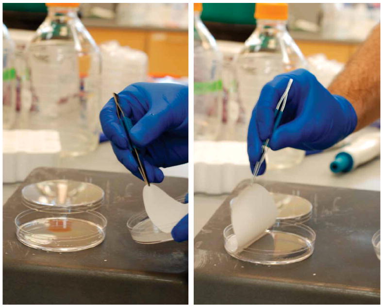
Quenching and extraction of a filter culture (Step 2A(x)). Removal of the filter culture from the agarose plate (left panel) and placement of the filter culture, cell side down, into the extraction solution (right panel).

Figure 7.

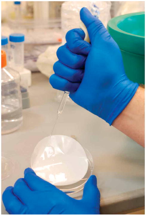
Rinsing the filter with extraction solution (Step 2A(xi)).

? TROUBLESHOOTING

● TIMING

It is important to note than many of these steps have times dependent upon the growth rate of the cell culture. As such, these times may vary substantially with your cultures.

• Step 1, making standards: 10–15 min per compound.

• Step 2A for E. coli:

  • Step (i): 15 min + 2 h to cool
  • Step (ii): overnight, 12–16 h
  • Steps (iii–iv): ~2 h
  • Steps (v–vii): ~2 min per culture
  • Step (viii): 2–3 h
  • Step (ix): 5 min + 15 min to cool
  • Steps (x–xix): ~1–2 h
• Step 2B for human fibroblasts:

  • Step (i): 15 min
  • Step (ii): 2–7 d
  • Step (iii): 10 min + 23 h
  • Step (iv): 10 min + 1 h
  • Steps (v–viii): 1 h

• Step 3: (optional) 3 h

• Steps 4–5: 15 min + LC-MS running time

• Steps 6–7: ~10 min per metabolite

• Steps 8–10: 10 min

• Step 11: 24 h for E. coli, 2–7 d for human fibroblasts

• Steps 12–13: 15 min

• Steps 14–16: (optional) 24 h for E. coli, 2–7 d for human fibroblasts

• Step 17–22: 1–2 h

? TROUBLESHOOTING

Lack of LC-MS signal

Check the LC-MS method to determine that settings are correct to detect compounds of interest. Concentrate sample to increase concentration.

Only a small fraction of metabolites are isotopically labeled

Allow cells to grow for more time in the labeled medium. Some cell lines may require additional labeled nutrients in addition to glucose and glutamine. If it is not possible to get near-complete isotopic labeling of a metabolite, the error may be reduced by increasing the concentration of standards used in determining R. This will decrease the value of R (by increasing its denominator), leading to smaller value of R_avgZ_avg, decreasing the contribution of the error from (1 − R_avgZ_avg) to the total error. We recommend keeping the value of R_avgZ_avg below 0.25.

Determination of L is cumbersome for some metabolites

In cases where unlabeled carbon can enter metabolism via only limited routes (e.g., bicarbonate), it is not necessary to determine L for every metabolite independently, as L must be equal for metabolites with the same carbon skeleton (e.g., glutamine, glutamate; NAD⁺, NADH; ADP, ATP) or containing the same carbon atoms (e.g., carbamoyl aspartate, dihydroorotate). For metabolites produced by unidirectional condensation of two substrates, L_product = L_substrate1 × L_substrate2 (e.g., L_{orotidine-5′-phosphate} = L_PRPP × L_orotate). These relationships eliminate the need to determine L for each species individually. They can also be used to reduce error in estimating L, by averaging across compounds for which L must be equal (e.g., NAD⁺, NADH).

ANTICIPATED RESULTS

Here, we go through one example of the calculation of the intracellular concentration of uridine-5′-triphosphate (UTP) in E. coli. Following Steps 1–7, the following peak heights for the ¹³C-labeled endogenous UTP and the ¹²C UTP standard were determined for four replicates:

	Sample no. 1	Sample no. 2	Sample no. 3	Sample no. 4
Plabeled	19,088	26,853	31,423	29,989
Punlabeled	8,895	12,590	21,218	22,778

Representative chromatograms (from Sample no. 2) are shown in Figure 8.

Figure 8.

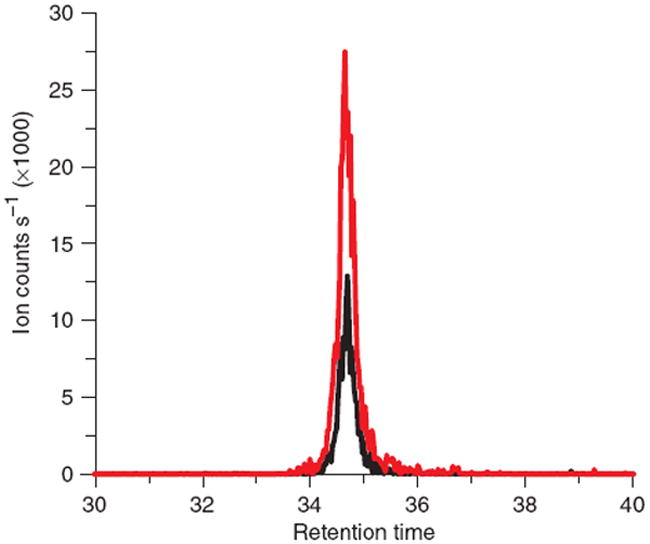
Representative extracted ion chromatograms of UTP. Signal is shown for unlabeled UTP arising from spiked standard (black) and for fully ¹³C-labeled UTP arising from endogenous E. coli metabolism (red). The observed signal intensities are used for the calculation of R in Step 8.

R_i is determined for each sample, with no. of carbons = 9, as described in Step 8:

	Sample no. 1	Sample no. 2	Sample no. 3	Sample no. 4
Ri	1.948	1.936	1.344	1.195

R_avg is calculated from the four values above, according to Step 9:

$$R_{\mathrm{avg}}=\exp \left(\frac{1}{4}\left(\ln 1.948+\ln 1.936+\ln 1.344+\ln 1.195\right)\right)=1.569$$

${\sigma }_{\ln R}^2$, the variance of R, is calculated according to Step 10:

$${\sigma }_{\ln R}^2=\frac{1}{3}\left({\left(\ln \frac{1.948}{1.569}\right)}^2+{\left(\ln \frac{1.936}{1.569}\right)}^2+{\left(\ln \frac{1.344}{1.569}\right)}^2+{\left(\ln \frac{1.195}{1.569}\right)}^2\right)=0.0630$$

For the calculation of L, the ratio of UTP peak sizes of ¹²C-glucose- to ¹³C-glucose-grown cultures was determined, as described in Step 11B:

	Sample no. 1	Sample no. 2	Sample no. 3	Sample no. 4
Punlabeled	23,800	22,200	27,700	19,100
Plabeled	12,200	14,700	14,100	12,800

L is determined for each sample, according to Step 11B, with no. of carbons = 9:

	Sample no. 1	Sample no. 2	Sample no. 3	Sample no. 4
Li	0.465	0.601	0.462	0.608

L_avg is calculated, according to Step 12:

$$L_{\mathrm{avg}}=\exp \left(\frac{1}{4}\left(\ln 0.465+\ln 0.601+\ln 0.462+\ln 0.608\right)\right)=0.530$$

This relatively small value of L is reasonable, as there are two separate reactions that can incorporate unlabeled carbonate into UTP: those catalyzed by carbamoyl-phosphate synthetase and phosphoenolpyruvate (PEP) carboxylase (which yields oxaloacetate, which forms aspartate and then condenses with carbamoyl phosphate to form carbamoyl aspartate, the committed compound of de novo pyrimidine biosynthesis).

${\sigma }_{\ln L}^2$ is calculated according to Step 13:

$${\sigma }_{\ln L}^2=\frac{1}{3}\left({\left(\ln \frac{0.465}{0.529}\right)}^2+{\left(\ln \frac{0.601}{0.529}\right)}^2+{\left(\ln \frac{0.462}{0.529}\right)}^2+{\left(\ln \frac{0.608}{0.529}\right)}^2\right)=0.0235$$

The total cellular volume of the culture, F, is calculated according to Step 17, based on the measured culture dry weight of 0.8 mg:

$$F=0.0008\mathrm{g}\times 0.0023L{\mathrm{g}}^{-1}=1.84\times {10}^{-6}L$$

C_avg is calculated from the above values according to Step 18, with Z determined to be zero in previous experiments¹⁷ and with S, the concentration of the internal standard in the first extraction step, equal to 8.28 × 10⁻⁷ M:

$$C_{\mathrm{avg}}=\frac{1.569}{0.530}\times \frac{\left(8.2\times {10}^{-7}\right)\times \left(2.5\times {10}^{-3}\right)}{1.84\times {10}^{-6}}=3.3\times {10}^{-3}\mathrm{M}$$

The variance of C_avg in logarithmic space, on the basis of variances of L and R, is calculated according to Step 18:

$${\sigma }_{\ln C}^2=0.0630+0.0235=0.0865$$

The standard error of C_avg, in logarithmic space, is calculated according to Step 20:

$${\mathit{SE}}_{\ln C}=\sqrt{\frac{0.0865}{4}}=0.147$$

The upper and lower bounds of the determined concentration are determined, according to Step 21:

$$\begin{array}{ll}{C}_{\mathrm{upper\; bound}}& =\exp \left(\ln \left(3.3\times {10}^{-3}\right)+1.96\times 0.147\right)\\ & =4.4\times {10}^{-3}\mathrm{M}\\ C_{\mathrm{lower\; bound}}& =\exp \left(\ln \left(3.3\times {10}^{-3}\right)-1.96\times 0.147\right)\\ & =2.5\times {10}^{-3}\mathrm{M}\end{array}$$

A final concentration of 3.3 mM UTP, with a 95% confidence interval of 2.5–4.4 mM, is reported.

References

- 1.Rabinowitz JD, Kimball E. Acidic acetonitrile for cellular metabolome extraction from Escherichia coli. Anal Chem. 2007;79:6167–6173. doi: 10.1021/ac070470c. [DOI] [PubMed] [Google Scholar]
- 2.Lu W, Kwon YK, Rabinowitz JD. Isotope ratio-based profiling of microbial folates. J Am Soc Mass Spectrom. 2007;18:898–909. doi: 10.1016/j.jasms.2007.01.017. [DOI] [PMC free article] [PubMed] [Google Scholar]
- 3.Yuan J, Fowler WU, Kimball E, Lu W, Rabinowitz JD. Kinetic flux profiling of nitrogen assimilation in Escherichia coli. Nat Chem Biol. 2006;2:529–530. doi: 10.1038/nchembio816. [DOI] [PubMed] [Google Scholar]
- 4.Lu W, Kimball E, Rabinowitz JD. A high-performance liquid chromatography-tandem mass spectrometry method for quantitation of nitrogen-containing intracellular metabolites. J Am Soc Mass Spectrom. 2006;17:37–50. doi: 10.1016/j.jasms.2005.09.001. [DOI] [PubMed] [Google Scholar]
- 5.Wu L, et al. Quantitative analysis of the microbial metabolome by isotope dilution mass spectrometry using uniformly 13C-labeled cell extracts as internal standards. Anal Biochem. 2005;336:164–171. doi: 10.1016/j.ab.2004.09.001. [DOI] [PubMed] [Google Scholar]
- 6.Mashego MR, et al. MIRACLE: mass isotopomer ratio analysis of U-C-13-labeled extracts. A new method for accurate quantification of changes in concentrations of intracellular metabolites. Biotechnol Bioeng. 2004;85:620–628. doi: 10.1002/bit.10907. [DOI] [PubMed] [Google Scholar]
- 7.Brauer MJ, et al. Conservation of the metabolomic response to starvation across two divergent microbes. Proc Natl Acad Sci USA. 2006;103:19302–19307. doi: 10.1073/pnas.0609508103. [DOI] [PMC free article] [PubMed] [Google Scholar]
- 8.Ikeda TP, Shauger AE, Kustu S. Salmonella typhimurium apparently perceives external nitrogen limitation as internal glutamine limitation. J Mol Biol. 1996;259:589–607. doi: 10.1006/jmbi.1996.0342. [DOI] [PubMed] [Google Scholar]
- 9.Rabinowitz JD. Cellular metabolomics of Escherchia coli. Expert Rev Proteomics. 2007;4:187–198. doi: 10.1586/14789450.4.2.187. [DOI] [PubMed] [Google Scholar]
- 10.Villas-Boas S, Bruheim P. Cold glycerol-saline: the promising quenching solution for accurate intracellular metabolite analysis of microbial cells. Anal Biochem. 2007;370:87–97. doi: 10.1016/j.ab.2007.06.028. [DOI] [PubMed] [Google Scholar]
- 11.Wittmann C, Kromer JO, Kiefer P, Binz T, Heinzle E. Impact of the cold shock phenomenon on quantification of intracellular metabolites in bacteria. Anal Biochem. 2004;327:135–139. doi: 10.1016/j.ab.2004.01.002. [DOI] [PubMed] [Google Scholar]
- 12.Villas-Boas SG, Hojer-Pedersen J, Akesson M, Smedsgaard J, Nielsen J. Global metabolite analysis of yeast: evaluation of sample preparation methods. Yeast. 2005;22:1155–1169. doi: 10.1002/yea.1308. [DOI] [PubMed] [Google Scholar]
- 13.Maharjan RP, Ferenci T. Global metabolite analysis: the influence of extraction methodology on metabolome profiles of Escherichia coli. Anal Biochem. 2003;313:145–154. doi: 10.1016/s0003-2697(02)00536-5. [DOI] [PubMed] [Google Scholar]
- 14.Kimball E, Rabinowitz JD. Identifying decomposition products in extracts of cellular metabolites. Anal Biochem. 2006;358:273–280. doi: 10.1016/j.ab.2006.07.038. [DOI] [PMC free article] [PubMed] [Google Scholar]
- 15.Meyer RC, et al. The metabolic signature related to high plant growth rate in Arabidopsis thaliana. Proc Natl Acad Sci USA. 2007;104:4759–4764. doi: 10.1073/pnas.0609709104. [DOI] [PMC free article] [PubMed] [Google Scholar]
- 16.Monton MR, Soga T. Metabolome analysis by capillary electrophoresis-mass spectrometry. J Chromatogr A. 2007;1168:237–246. doi: 10.1016/j.chroma.2007.02.065. discussion 236. [DOI] [PubMed] [Google Scholar]
- 17.Bajad SU, et al. Separation and quantitation of water soluble cellular metabolites by hydrophilic interaction chromatography-tandem mass spectrometry. J Chromatogr A. 2006;1125:76–88. doi: 10.1016/j.chroma.2006.05.019. [DOI] [PubMed] [Google Scholar]
- 18.Tolstikov VV, Lommen A, Nakanishi K, Tanaka N, Fiehn O. Monolithic silica-based capillary reversed-phase liquid chromatography/electrospray mass spectrometry for plant metabolomics. Anal Chem. 2003;75:6737–6740. doi: 10.1021/ac034716z. [DOI] [PubMed] [Google Scholar]
- 19.Maruska A, Rocco A, Kornysova O, Fanali S. Synthesis and evaluation of polymeric continuous bed (monolithic) reversed-phase gradient stationary phases for capillary liquid chromatography and capillary electrochromatography. J Biochem Biophys Methods. 2007;70:47–55. doi: 10.1016/j.jbbm.2006.10.011. [DOI] [PubMed] [Google Scholar]
- 20.Horie K, et al. Highly efficient monolithic silica capillary columns modified with poly(acrylic acid) for hydrophilic interaction chromatography. J Chromatogr A. 2007;1164:198–205. doi: 10.1016/j.chroma.2007.07.012. [DOI] [PubMed] [Google Scholar]
- 21.Wilson ID, et al. HPLC-MS-based methods for the study of metabonomics. J Chromatogr B Analyt Technol Biomed Life Sci. 2005;817:67–76. doi: 10.1016/j.jchromb.2004.07.045. [DOI] [PubMed] [Google Scholar]
- 22.Nguyen DT, et al. High throughput liquid chromatography with sub-2 microm particles at high pressure and high temperature. J Chromatogr A. 2007;1167:76–84. doi: 10.1016/j.chroma.2007.08.032. [DOI] [PubMed] [Google Scholar]
- 23.Guillarme D, Nguyen DT, Rudaz S, Veuthey JL. Method transfer for fast liquid chromatography in pharmaceutical analysis: application to short columns packed with small particle. Part I: isocratic separation. Eur J Pharm Biopharm. 2007;66:475–482. doi: 10.1016/j.ejpb.2006.11.027. [DOI] [PubMed] [Google Scholar]
- 24.Yu K, Little D, Plumb R, Smith B. High-throughput quantification for a drug mixture in rat plasma—a comparison of ultra performance liquid chromatography/tandem mass spectrometry with high-performance liquid chromatography/tandem mass spectrometry. Rapid Commun Mass Spectrom. 2006;20:544–552. doi: 10.1002/rcm.2336. [DOI] [PubMed] [Google Scholar]
- 25.Cai SS, Hanold KA, Syage JA. Comparison of atmospheric pressure photoionization and atmospheric pressure chemical ionization for normal-phase LC/MS chiral analysis of pharmaceuticals. Anal Chem. 2007;79:2491–2498. doi: 10.1021/ac0620009. [DOI] [PubMed] [Google Scholar]
- 26.Hu Q, et al. The Orbitrap: a new mass spectrometer. J Mass Spectrom. 2005;40:430–443. doi: 10.1002/jms.856. [DOI] [PubMed] [Google Scholar]
- 27.Wilson SD, Horne DW. Evaluation of ascorbic acid in protecting labile folic acid derivatives. Proc Natl Acad Sci USA. 1983;80:6500–6504. doi: 10.1073/pnas.80.21.6500. [DOI] [PMC free article] [PubMed] [Google Scholar]
- 28.Luo B, Groenke K, Takors R, Wandrey C, Oldiges M. Simultaneous determination of multiple intracellular metabolites in glycolysis, pentose phosphate pathway and tricarboxylic acid cycle by liquid chromatography-mass spectrometry. J Chromatogr A. 2007;1147:153–164. doi: 10.1016/j.chroma.2007.02.034. [DOI] [PubMed] [Google Scholar]
- 29.van Winden WA, et al. Metabolic-flux analysis of Saccharomyces cerevisiae CEN.PK113-7D based on mass isotopomer measurements of 13C-labeled primary metabolites. FEMS Yeast Res. 2005;5:559–568. doi: 10.1016/j.femsyr.2004.10.007. [DOI] [PubMed] [Google Scholar]
- 30.Coulier L, et al. Simultaneous quantitative analysis of metabolites using ion-pair liquid chromatography-electrospray ionization mass spectrometry. Anal Chem. 2006;78:6573–6582. doi: 10.1021/ac0607616. [DOI] [PubMed] [Google Scholar]
- 31.Brown AF, Dunn GA. Microinterferometry of the movement of dry matter in fibroblasts. J Cell Sci. 1989;92(Part 3):379–389. doi: 10.1242/jcs.92.3.379. [DOI] [PubMed] [Google Scholar]