Cue-Invariant Networks for Figure and Background Processing in Human Visual Cortex

Abstract

Lateral occipital cortical areas are involved in the perception of objects, but it is not clear how these areas interact with first tier visual areas. Using synthetic images portraying a simple texture-defined figure and an electrophysiological paradigm that allows us to monitor cortical responses to figure and background regions separately, we found distinct neuronal networks responsible for the processing of each region. The figure region of our displays was tagged with one temporal frequency (3.0 Hz) and the background region with another (3.6 Hz). Spectral analysis was used to separate the responses to the two regions during their simultaneous presentation. Distributed source reconstructions were made by using the minimum norm method, and cortical current density was measured in a set of visual areas defined on retinotopic and functional criteria with the use of functional magnetic resonance imaging. The results of the main experiments, combined with a set of control experiments, indicate that the figure region, but not the background, was routed preferentially to lateral cortex. A separate network extending from first tier through more dorsal areas responded preferentially to the background region. The figure-related responses were mostly invariant with respect to the texture types used to define the figure, did not depend on its spatial location or size, and mostly were unaffected by attentional instructions. Because of the emergent nature of a segmented figure in our displays, feedback from higher cortical areas is a likely candidate for the selection mechanism by which the figure region is routed to lateral occipital cortex.

Introduction

Object recognition mechanisms must be able to extract shape independently of the surface cues that are present. Local estimates of surface cues such as texture grain or orientation, although necessary as inputs to the recognition process, convey little sense of object shape. Rather it is the pattern of cue similarity across regions and cue discontinuity across borders that must be integrated to recover object shape.

The process of cue-invariant shape processing begins at an early stage of visual cortex and extends deep into extrastriate cortex and the temporal lobe. Cue invariance first is seen as early as V2, where some cells have a similar orientation or direction tuning for borders defined by different feature discontinuities (Leventhal et al., 1998; Marcar et al., 2000; Ramsden et al., 2001; Zhan and Baker, 2006). At higher levels of the visual system, such as inferotemporal cortex (Sary et al., 1993) and medial superior temporal area (Geesaman and Andersen, 1996), cells show shape selectivity that is mostly independent of the defining cues and spatial position. Functional magnetic resonance imaging (fMRI) studies in humans have implicated homologous extrastriate regions, in particular the lateral occipital complex (LOC), as sites of category-specific, cue-invariant object processing (Grill-Spector et al., 1998; Vuilleumier et al., 2002; Marcar et al., 2004).

Beyond cue-independent border processing in V2, late responses in V1 have been reported to be larger when the receptive field is covered by the figure region of figure/ground displays, defined by differences in the orientation or direction of motion of textures in the figure versus background regions (Zipser et al., 1996; Lee et al., 1998; Lamme et al., 1999) or by the borders of an illusory figure (Lee and Nguyen, 2001). Response modulations by figure/background displays seen in early areas may not, however, represent a fully elaborated figure/background mechanism, because they depend on stimulus size and position (Zipser et al., 1996; Rossi et al., 2001) and occur for stimuli that do not represent closed regions and therefore do not segregate perceptually (Rossi et al., 2001). Modulation is also weak with a cue (discontinuity of iso-oriented textures) that does support segmentation (Marcus and Van Essen, 2002). Processing in V1 (and V2) therefore may represent a precursor stage of full figure/background.

Although the available evidence suggests that object segmentation involves multiple levels of processing, existing single unit studies have, with one exception (Lee et al., 2002), recorded in only a single area in any one study, and fMRI studies either have focused on early visual areas (Schira et al., 2004; Scholte et al., 2006) or have found activation only in higher cortical areas such as LOC (Grill-Spector et al., 1998; Kastner et al., 2000). To address which areas are involved in figure/ground processing and the timing of responses in the network, we have developed an EEG source-imaging procedure that separately tracks figure and background responses on the cortical surface. Using this approach, we found that the LOC preferentially represents the figure rather than the background region in a manner that is mostly invariant with respect to cue type, size, and position.

Materials and Methods

Participants

A total of 13 observers participated in these experiments (mean age 36). All participants had visual acuity of better than 6/6 in each eye, with correction if needed, and stereoacuity of 40 arc s or better on the Titmus and Randot stereoacuity tests. Acuity was measured with the Bailey–Loeve chart, which has five letters per line and equal log increments in the letter sizes across lines. Informed consent was obtained before experimentation under a protocol that was approved by the Institutional Review Board of the California Pacific Medical Center. All 13 observers participated in the main experiment, whereas five observers participated in the spatial and attention control experiments.

Stimulus construction and frequency-tagging procedure

Main experiment. Stimulus generation and signal analysis were performed by in-house software, running on the Power Macintosh platform. Stimuli were presented on a Sony (Tokyo, Japan) multi-synch video monitor (GDP-400) at a resolution of 800 × 600 pixels, with a 72 Hz vertical refresh rate. The nonlinear voltage versus luminance response of the monitor was corrected in software after calibration of the display with an in-house linear positive-intrinsic-negative (PIN) diode photometer equipped with a photopic filter. Participants were instructed to fixate on a fixation mark at the center of the display and to distribute attention evenly over the entire display. The monitor was positioned 59 cm from the observer, and stimuli were viewed in a dark and quiet room. Individual trials lasted 16.7 s, and conditions were randomized within a block. A typical session lasted ∼1 h and consisted of 10–15 blocks of randomized trials in which the observer paced the presentation and was given opportunity to rest between blocks.

In our displays “figure” and “background” regions were tagged with different temporal frequencies to study surface segmentation based on similarities and differences in elementary features. The textures comprising both figure and background regions consisted of one-dimensional random luminance bars or single pixel elements. The minimum bar or pixel width was 6 arc min, and the maximum contrast between elements was 80%, based on the Michelson definition as follows:

where L_max and L_min are the maximum and minimum bar luminance in the stimulus. The mean luminance was 56.3 cd/m², and the full display subtended 21 by 21° of visual angle.

The stimuli were designed such that the textures composing the figure and background regions modulated at different temporal frequencies. Evoked responses thus were forced to occur at exact integer multiples of these modulation frequencies, which are referred to as “frequency tags.” Figure 1A–C illustrates three types of texture cues that were used in the main experiment. Four stimulus frames constituting the different stimulus configurations that occur within a single presentation cycle are displayed for each cue type. Although the individual components modulate periodically, the alternation between segmentation states does not follow a simple time course and is periodic only on the scale of the full 1.67 s stimulus cycle (Fig. 1D). The top line in Figure 1D represents the background modulation occurring at 3.6 Hz (f2). The bottom line represents the figure modulation occurring at 3.0 Hz (f1). Intervals in which the figure and background regions are segmented from each other are shaded gray and labeled with an “S.” Occurrences of the four frames illustrated in Figure 1A–C are indicated with arrows.

Figure 1.

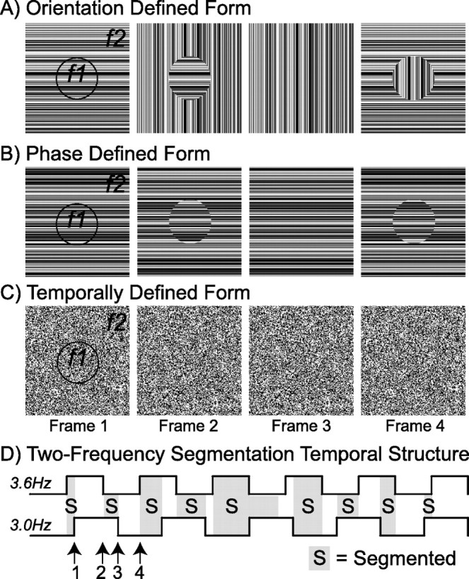
Schematic illustration of three segmentation cues. Texture-defined stimuli composed of a central 5° figure region and a 21 ×21° background region were defined on the basis of periodic frequency tags applied to each region. In all conditions, the figure region was tagged at 3.0 Hz (f1) and the background region at 3.6 Hz (f2). Four characteristic frames are shown for each of three cues used to define figure/background segmentation in this experiment. A, Orientation-defined form in which the figure and background textures each changed orientation by 90°. B, Phase-defined form in which the textures alternated phase (180° rotation, flipping about the midline). C, Temporally defined form (TDF) in which random luminance square elements containing no orientation information were updated at the figure and background frequency tags. Additional control conditions (data not shown) consisted of an orientation modulating figure presented in isolation on a mean gray background (3.0 Hz) and a full field texture rotating by 90° at 3.6 Hz. D, A schematic representation of the temporal structure of figure segmentation over one full stimulus cycle (1.67 s). In this illustration, the states of the background (top square wave) and the figure (bottom square wave) are depicted by the solid lines. The sequence of figure segmentation resulting from these modulations is indicated by the shaded gray (segmented) and white (unsegmented) areas, with numbered arrows indicating the onset of individual frames (1–4), shown above.

The alternation between segmented and uniform states is depicted by the four frame types of the orientation-defined form condition in Figure 1A. In this stimulus a circular 5° diameter region, centered on fixation, changed orientation by 90° at 3.0 Hz. The background texture changed orientation by 90° at 3.6 Hz. Because the figure and background regions change at different rates, the texture cycles through four states; the display begins with the figure and background both aligned horizontally. After 138 ms the background switches orientation, and the figure region (horizontal texture) segments from the vertical background. When the figure region subsequently switches to the vertical orientation, the figure disappears; finally, when the background region switches from vertical to horizontal, the segmentation is reestablished. The figure exists only when the two regions are of dissimilar orientation, and the segmentation disappears when they are both in alignment. Thus the figure region is cued by both a difference in orientation and by a difference in the frequencies of the tags imposed on the two regions.

Using the same frequency tagging design, we created a second stimulus in which the figure was defined by local contrast discontinuities at the border of horizontally oriented figure and background textures (Fig. 1B). We will refer to this stimulus as the phase-defined form for brevity. In practice, these stimuli were generated by rotating the figure and background regions by 180° (flipping about the midline). Because the orientation of the figure and background regions was always horizontal, the segmentation was defined by spatiotemporal luminance discontinuities along the length of the bars that occurred at the figure/background border.

Finally, by using random luminance square elements (6 arc min on a side), we removed orientation information altogether, forcing the segmentation process to rely solely on the two different temporal tags. Despite the lack of orientation information, this stimulus supports the appearance of a segmented disk on a uniform background. Four frames of the temporally defined form condition are shown in Figure 1C. Unlike the case of the orientation- and phase-defined stimuli in which any single frame of the display can be classified as either segmented or not, single frames of the temporally defined form are always spatially uniform, and the segmentation information presumably is carried by the detection of temporal asynchrony between the two regions. Because the segmentation is based purely on temporal asynchrony of the two regions, the figure region does not segment from the background in these static depictions. The temporally defined form also was generated by image rotation, with the figure region rotating at 3.0 Hz and the background at 3.6 Hz. Animations of the stimuli are provided in the supplemental material (available at www.jneurosci.org).

In addition to the stimuli previously described, two conditions containing only a single frequency tag were included to assess the responses to the figure and background alone in the absence of segmentation appearance and disappearance resulting from their interactions. In the figure-only condition the figure region was presented on a mean gray background containing no texture. In this stimulus the figure alternated orientation by 90° at 3.0 Hz. The figure size and shape were the same as in the other conditions, but here the figure segmentation was continuous and defined by a difference in contrast (0 vs 80%) and temporal frequency (0 vs 3.0 Hz). In the full field condition the entire field (21 by 21°) was made to alternate orientation by 90° at 3.0 Hz. Here no figure was present other than that defined by the edges of the display.

Test of spatial and size invariance.

A separate experimental session was run to evaluate the influence of the spatial position and figure size on the figure region response. Spatial invariance was assessed by presenting a 2° diameter phase-defined form stimulus centered at −4, −2, 0, 2, and 4° eccentricity from the fixation point along the horizontal meridian (see Fig. 7A). Participants again were instructed to fixate on the fixation mark and distribute attention evenly over the whole display. In total, 20 trials were run at each fixation locus. By contrasting responses at the five fixations, we were able to evaluate the influence of visual field position on figure-related activity. We assessed the influence of figure size by comparing responses to the centrally presented 2° stimulus with those from the 5° stimulus of the main experiment (within the five observers who participated in both experiments).

Figure 7.

Test of spatial invariance. A, So that the influence of spatial position on cortical responses could be evaluated, a 2° phase-defined form stimulus was viewed as participants fixated on one of five fixation points (indicated with stars) spaced at 2° intervals across the horizontal midline (note that the actual stimulus extends to 21 × 21°). B, Figure (solid) and background (dashed) response values from the LOC ROI are shown separately for the left (dark) and right (light) hemispheres at each fixation location. The LOC ROI displays considerable contralateralization. When the figure falls in the left visual field, figure responses are largest in the right LOC ROI; conversely, when the figure falls in the right visual field responses are largest in the left LOC ROI. Within a hemifield, the response magnitudes differ by 6 and 3% (relative to the maximum) for the left and right hemispheres, respectively. The background responses mostly are unaffected by the fixation location. C, Spline-interpolated scalp voltage topographies are shown for the second harmonic of the figure (top) and background (bottom) at each fixation location.

Test of attentional influence.

To assess the influence of attention on the amplitude and timing of brain responses involved in figure versus background processing, we performed a separate experimental session with five of the observers from the main experiment. This session consisted of two experimental conditions in which two different tasks were added to the orientation-defined form stimulus described in the main experiment. In separate blocks of trials one of two instructions was given to the observers. In the “attend configuration” trials the observers indicated a change in the shape of the figure by pressing a mouse key. On 20% of the 1.67 s stimulus cycles the aspect ratio of the figure became elliptical (see Fig. 4E, schematic illustration). Responses were monitored, and the figure aspect ratio was adjusted to maintain performance at ∼80% correct detection. In the “attend letter” trials the observers were instructed to attend to a stream of simultaneously presented letters and to detect a probe letter “T” among distracters “L.” Letter arrays containing Ls and Ts appeared superimposed on the figure region of the stimulus (see 4F, schematic illustration) and were preceded and followed by masking arrays of only “F”s. A staircase procedure was used to maintain a constant high level of task difficulty by holding performance at or near the duration threshold for letter detection. The duration of presentation was decreased with each correct response and lengthened with each incorrect response according to an adaptive rule that converged on the 82% correct level of the psychometric function. Four repetitions of these tasks were performed while the orientation-defined form stimulus was presented continuously for 2 min. Both tasks were present on the screen at the same time, and only the instructions given to the observers differed.

Figure 4.

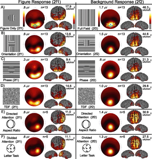
Group-averaged responses for the figure (2f1) and background (2f2) are shown for each of the four cue types (A–D) and two attention conditions (E, F). Topographies and current density estimates are shown as 13 subject grand averages for the second harmonic of the figure on the left and the background on the right. Figure responses are lateralized over the occipital cortex for all cues and attention conditions. Background responses are focused on the midline pole and are similar for all cue types and attention conditions. A schematic illustration of each stimulus, the number of observers included in the average, and the response maximum are included for each response distribution. The seven channel locations (Electrical Geodesics HydroCell Sensor Net, channels 59, 65, 71, 72, 75, 76, 90, 91) used to test sensor map differences are superimposed on the two-dimensional maps for the figure-only and full field. They are coded blue for the medial channels (Oz) and green for the lateral channels (P7 and P8).

EEG signal acquisition

The EEG was collected with a whole-head, 128-channel geodesic EEG system with HydroCell Sensor Nets (Electrical Geodesics, Eugene, OR). This system provides uniform spatial sampling (∼2 cm sensor to sensor), covering the entire scalp surface and extending 120° in all directions from the vertex reference electrode. The EEG was amplified at a gain of 1000 and recorded with a vertex physical reference. Signals were 0.1 Hz high-pass-filtered and 50.0 Hz (Bessel) low-pass-filtered and were digitized at 432 Hz with a precision of 4 bits/μV at the input. The 16-bit analog-to-digital converter was clocked externally via a hardware interface to the video card that used the horizontal synch of the video monitor as its base clock. The sampling rate was derived by downcounting an integer number of video lines to yield exactly six samples per video frame. The video stimulation computer also sent a digital trigger mark to the recording system at the top of the first active video frame to indicate the precise beginning of the trial.

After each experimental session the three-dimensional (3-D) locations of all electrodes and the three major fiducials (nasion and left and right peri-auricular points) were digitized by a 3Space Fastrack 3-D digitizer (Polhemus, Colchester, VT). In instances in which MRI scans were collected on participants, the 3-D digitized locations were used to coregister the electrodes to the anatomical scans.

Artifact rejection and spectral analysis of EEG data were done off-line. Artifact rejection proceeded in two steps. First, raw data were evaluated on a sample-by-sample basis to determine the number of individual samples exceeding a prescribed threshold (∼25–50 μV). Noisy channels, i.e., those containing a large percentage of samples exceeding threshold, were replaced by the average of the six nearest spatial neighbors. Typically, only two to four channels were substituted. Next, using the same sample-by-sample evaluation, we marked EEG epochs that contained a large percentage of data samples exceeding threshold (∼25–50 μV) for exclusion on a channel-by-channel basis. Here epoch was defined as a single period of the total stimulus cycle or 1.67 s, which equates to the least common multiple of the figure and background periods.

Once noisy channels were substituted and artifactual epochs were excluded, the EEG was re-referenced to the common average of all of the channels. Time averages for each stimulus condition were computed over one stimulus cycle (1.67 s). Next the time averages were converted to complex-valued amplitude spectra at a frequency resolution of 0.6 Hz via a discrete Fourier transform. Then the resulting amplitude spectra of the steady-state visually evoked potential (SSVEP) were evaluated at discrete frequencies uniquely attributable to the input stimulus frequency tags up to the 18th and 15th harmonic for the figure and background tags, respectively.

Head conductivity modeling

Our source localization procedure used a boundary element model (BEM; EMSE Suite software, Source Signal Imaging, San Diego, CA) of the electrical conductivity of the individual observers' heads. In separate MRI sessions T1 whole-head anatomical MRI scans were collected from 11 of the 13 observers on a 3T General Electric Signa LX scanner, using a 3-D SPGR or MP-RAGE pulse sequence. All anatomical head volumes were composed of sagittal slices, acquired with a resolution of 0.94 × 0.94 × 1.2 mm or better. For each observer one to three whole-brain T1-weighted anatomical data sets were acquired. These images were aligned, averaged, and resampled into a 1 × 1 × 1 mm resolution 3-D anatomical volume that was corrected for inhomogeneities by using the FSL (fMRI of the Brain Software Library) toolbox (http://www.fmrib.ox.ac.uk/fsl/).

Head models were based on compartmentalized tissue segmentations that defined contiguous regions for the scalp, outer skull, inner skull, and the cortex. First, approximate cortical tissue volumes for gray and white matter were defined by voxel intensity thresholding and anisotropic smoothing via the EMSE package. The resulting white matter and pial tissue boundaries were used to extract the contiguous cortical gray matter surface. Using the cortical gray matter, we then ran an expansion algorithm to derive the inner and outer surfaces of the skull. Then the scalp surface was determined by removing extraneous extra-scalp noise and defining the surface with a minimum imposed thickness. Last, the scalp, skull, and brain regions were bounded by surface tessellation, and all tissue surface tessellations were checked visually for accuracy to ensure that no incidental intersection had occurred between concentric meshes. Coregistration of the electrode positions to the MRI head surface was done by alignment of the three digitized fiducial markers with their visible locations on the anatomical head surface. Final adjustments were completed by using a least-squares fit algorithm, and electrode deviations from the scalp surface were removed.

Cortically constrained minimum norm source estimates

The spatiotemporal distribution of neural activity underlying the measured EEG signals was modeled with the cortically constrained minimum norm procedure of the EMSE package. This technique assumes that surface EEG signals are generated by multiple dipolar sources that are located in the gray matter and oriented perpendicular to the cortical surface. Because the precise shape of the cortex is critical in determining the cortical source generators, we replaced the rapid surface segmentation produced by EMSE with a more accurate segmentation of the cortical surface generated with the FreeSurfer software package (http://surfer.nmr.mgh.harvard.edu). This segmentation generated a representation of the pial surface, and the segmentation was checked (and hand-edited if necessary) by a human expert. This cortical surface mesh was reintegrated with the scalp and skull meshes within the EMSE package before the construction of the BEMs and data visualization on the cortical surface

In the minimum norm procedure cortical current density (CCD) estimates are determined by a linear optimization of dipole magnitudes (Hamalainen and Ilmoniemi, 1994). This produces a continuous map of current density on the cortical surface having the least total (RMS, root mean square) power while still being consistent with the voltage distribution on the scalp. In addition, the EMSE implementation uses lead field normalization to compensate for the inherent bias toward superficial sources of the unweighted minimum norm inverse (Lin et al., 2006).

Visual area definition by fMRI retinotopic mapping

fMRI scans were collected on very similar 3T General Electric scanners located at either the Stanford Lucas Center (Stanford, CA) or the University of California, San Francisco (UCSF) China Basin Radiology Center. Data from Stanford were acquired with a custom whole-head two-channel coil or a two-channel posterior head surface coil and a spiral K-space sampling pulse sequence. At UCSF a standard General Electric eight-channel head coil was used, together with an EPI (echo-planar imaging) sequence. Despite slight differences in hardware and pulse sequence, the data quality from the two sites was very similar. The general procedures for these scans (head stabilization, visual display system, etc.) are standard and have been described in detail previously (Brewer et al., 2005; Tyler et al., 2006). Retinotopic field mapping produced regions of interest (ROIs) defined for each participant's visual cortical areas V1, V2v, V2d, V3v, V3d, V3a, and V4 in each hemisphere (DeYoe et al., 1996; Tootell and Hadjikhani, 2001; Wade et al., 2002). ROIs corresponding to each participant's human middle temporal area (hMT+) were identified, using low-contrast motion stimuli similar to those described by Huk et al. (2002).

The LOC was defined in one of two ways. For four participants the LOC was identified by using a block design fMRI localizer scan. During this scan the observers viewed blocks of images depicting common objects (18 s/block) alternating with blocks containing scrambled versions of the same objects. The stimuli were those used in a previous study (Kourtzi and Kanwisher, 2000). The regions activated by these scans included an area lying between the V1/V2/V3 foveal confluence and hMT+ that we identified as the LOC.

The LOC is bounded by retinotopic visual areas and area hMT+. For observers without a LOC localizer, we defined the LOC on flatted representations of visual cortex as a polygonal area with vertices just anterior to the V1/V2/V3 foveal confluence, just posterior to area hMT+, just ventral to area V3B, and just dorsal to area V4. This definition covers almost all of the regions (e.g., V4d, lateral occipital cortex, lateral occipital peripheral area) that previously have been identified as lying within the object-responsive lateral occipital cortex (Malach et al., 1995; Kourtzi and Kanwisher, 2000; Tootell and Hadjikhani, 2001) and none of the standard “first tier” retinotopic visual areas.

ROI SSVEP quantification

SSVEPs were analyzed separately to extract the magnitude and the time course of responses from the figure and background regions within each retinotopically or functionally defined ROI. ROI-based analysis of the EEG data was performed by extending the Stanford VISTA toolbox (http://white.stanford.edu/software/) to accept EMSE-derived minimum norm inverses, which in turn were combined with the cycle-averaged EEG time courses to obtain CCD time series activation maps.

An estimate of the average response magnitude for each ROI was computed as follows. First, the complex-valued Fourier components for each unique response frequency were computed for each mesh vertex. Next, a single complex-valued component was computed for each ROI by averaging across all nodes within that ROI (typically > 300). This averaging was performed on the complex Fourier components and therefore preserved phase information. Averaging across hemispheres and observers then was performed for each individual frequency component. This averaging also maintained the complex phase of the response. Finally, for each ROI the total amplitude of the first, second, third, fourth, and eighth harmonics was computed for both the figure and background frequency tags, using the following formula:

where z_j denotes the complex Fourier coefficient of the jth harmonic, and an asterisk denotes its complex conjugate. This operation is equivalent to summing the powers of the individual harmonics and then taking the square root. The relative phases of the individual harmonics thus do not contribute to the final magnitude estimate. Real and imaginary terms of each complex-valued variance around the mean of each harmonic (across observers) were propagated via this formula to obtain SEs of the total amplitudes for each ROI (Bevington and Robinson, 1992) as follows:

where μ and σ denote the mean and SD of each term (real or imaginary) from each of the harmonics in the sum, and n denotes the number of subjects. One frequency (18 Hz) was a common multiple of the two tag frequencies (6f1 and 5f2) and was not included.

The time course of activity elicited by the figure and background regions was computed by selectively back-transforming either the figure (nf1) or background (nf2) harmonics up to 54 Hz. Again, components that could be attributed to both figure and background were excluded (e.g., 18, 36, and 54 Hz). This inverse transformation acts as a filter that enables examination of the temporal evolution of the SSVEP while allowing interpretation separately for signals generated by the two stimulus frequency tags. The resulting waveforms reflect a single cycle of the figure or background fundamental frequency, respectively.

Statistical analysis

SSVEP significance.

The statistical significance of the harmonic components of each observer's single condition data was evaluated by using the T²-Circ statistic (Victor and Mast, 1991). This statistic uses both amplitude and phase consistency across trials to asses whether stimulus-locked activity is present.

Multivariate analysis of variance.

Differences among experimental design factors of region, cue, attention condition, and figure size were assessed by using a multivariate approach to repeated measures (multivariate analysis of variance, MANOVA) that takes into account the correlated nature of repeated measures (for review, see Keselman et al., 2001). MANOVA was performed in one of two ways. To assess differences in voltage distributions on the scalp, we performed MANOVA on the second harmonic responses of the figure and background regions, using a subset of sensor locations corresponding to Oz, P7, and P8 in the International 10-20 System. These sensors were identified from an independent data set obtained from a pilot study. To evaluate differences in source distribution corresponding to stimulus condition or region, we also performed MANOVA on the total spectral magnitude in source space for each ROI. For each instantiation of MANOVA in our design, the specific design factors and levels are described in the appropriate section in Results.

Waveform permutation testing.

Differences between source waveforms were identified by a permutation test based on methods devised by Blair and Karniski (1993). For any two waveforms A and B, let Y_A and Y_B, respectively, denote the t-by-n matrices of current density, in which n denotes the number of subjects and t the number of samples in each waveform. First, we define the t-by-n difference waveform matrix, ΔY = Y_A –Y_B, so that the individual columns, ΔY_i, i = 1,…,n, represent for each subject the difference between the two waveforms. Then we compute the following statistics:

the t-by-1 mean difference waveform vector,

the t-by-1 variance vector, and

the t-by-1 vector of t scores.

From the third vector we determine the longest consecutive sequence of t scores having p values < 0.05. The number of time points in this longest sequence is denoted T_LSS.

The null hypothesis of no difference between A and B implies that each observer's waveforms are exchangeable. Therefore, the signs of the columns ΔY_i, i = 1,..,n can be chosen at random to obtain a permutation sample, ΔY*, from which we can calculate a corresponding t score vector, T*_ΔY, and its longest sequence length, T*_LSS. Considering every possible permutation of sign for the columns (subjects) of ΔY, we accumulate a permutation sample space of ΔY* and a nonparametric reference distribution for T*_LSS. We then determine the critical value, T_C, that is >95% of the values in the reference distribution of T*_LSS.

We rejected the null hypothesis if the length of any consecutive sequence of significant t scores in the original, nonrandomized data exceeded T_C. Because each permutation sample contributes only its longest significant sequence to the reference distribution, the null hypothesis predicts exactly a 5% chance that any T_LSS > T_C. Therefore, this procedure implicitly compensates for the problem of multiple comparisons and is a valid test for the omnibus hypothesis of no difference between the waveforms at any time point. Furthermore, this test not only detects significant departures from the null hypothesis, it also localizes the time periods when such departures occur.

Source space CCD averages and animations

To create average spatiotemporal maps of activity on the cortical surface, we performed a group analysis first by averaging the filtered waveforms (see above) for all 13 subjects in sensor space. Averaged data then were referenced to the electrode positions of an individual participant, and CCD maps were created from that individual's minimum norm estimates. In this way the average activity for the figure and background regions could be visualized as animations for each stimulus condition (see supplemental material, available at www.jneurosci.org).

Results

The goal of this study is to visualize the evolution of figure and background region responses over cortical areas and time and to establish whether these responses depended on the stimulus configuration or attentional state of the observer. We begin with a “sensor space” analysis (voltage as a function of electrode location) in the frequency domain in which we demonstrate our main effects and establish that these responses are robust to attentional instruction. We then provide a “source space” (cortical surface current density reconstruction) frequency domain analysis, first in individual functionally defined visual areas for several representative observers and then as group averages. We show the spatiotemporal evolution of region-tagged signals through cortex by performing a time domain analysis in source space. As in the sensor space analyses, we also demonstrate our main effects in source space, and we also establish size and position invariance. Finally, to visualize the temporal evolution of these responses over the cortex, we present animations of the separate figure and background region responses in the supplemental material (available at www.jneurosci.org).

Figure and background region response spectra

In all stimulus conditions and for all participants the SSVEPs were present at harmonics of the frequency tags and at frequencies equal to low-order sums and differences of the two tag frequencies. Typically, the largest responses were observed at the second harmonic (2f) of each frequency tag, in which f is the tagging frequency. The image-updating procedure produces two temporal transients for each cycle of the figure region animation (e.g., 0–90° and 90–0° for the orientation-defined form), and it thus is not surprising that a large response would be evoked at the second harmonic. The observation that the responses are dominated by even harmonics of the tag frequencies indicates that the responses to each stimulus transition evoke similar responses in the population.

Statistically significant responses extended to the highest recorded frequencies (54 Hz), with 79.7% of the sensors located over the occipital cortex having T²-Circ p values < 0.05 at the first four harmonics of each frequency tag. Example amplitude spectra from an individual observer, recorded at representative sensors located over the visual cortex, are shown in Figure 2. The spectra are displayed above two frames of the stimulus from which they were generated. In Figure 2A the figure-only condition is illustrated. In this condition only the figure region is presented, and SSVEP responses are observable as spikes in the spectrum (shaded bars) occurring at integer multiples of the frequency tag (3.0, 6.0, 9.0 Hz…). Figure 2B shows the amplitude spectrum and stimulus frames from the full field condition. In this condition the same frequency tag is applied to the full texture field, and responses are again present at integer multiples of the tag frequency.

Figure 2.

Steady-state responses for three stimulus conditions. Amplitude spectra of one observer are depicted for a representative EEG sensor located over the response maxima [sensors 85 (A, C) and 75 (B) of the Geodesics HydroCell Sensor Net] for three stimulus conditions: figure-only (A), full field (B), and the orientation-defined form (C). Each amplitude spectrum is located over two frames of the stimulus from which it was obtained. SSVEP responses were present at integer multiples of the stimulus frequencies for each stimulus condition. Responses at harmonics of the stimulus frequencies are shown as darkened lines, with corresponding labels (nF1, figure-related; nF2, background-related). The figure-only stimulus condition (A) produced responses at integer multiples of the figure frequency tag (3.0, 6.0, 9.0 Hz…). Responses to the full field stimulus condition (B) were present at the harmonics of the full field frequency tag (3.0, 6.0, 9.0 Hz…). The amplitude spectrum resulting from the orientation-defined form stimulus (C) contained responses at harmonics of both the figure (3.0, 6.0, 9.0 Hz…) and the background (3.6, 7.2, 10.8 Hz…) tags as well as at low-order sums and the difference of these two frequencies (0.6, 6.6 Hz…).

Figure 2C shows two frames of the orientation-defined form stimulus and the amplitude spectrum of the corresponding response. Separately identifiable SSVEP responses are present at harmonics of both the figure tag frequency (3.0, 6.0, 9.0 Hz…) and the background tag frequency (3.6, 7.2, 10.8 HZ…) during the simultaneous presentation of both regions. In addition, responses (illustrated by the light bars) are present at frequencies equal to low-order sums and differences of the two input frequencies (e.g., 0.6, 6.6 Hz…). These components are attributable to nonlinear interaction between figure and background regions and will be discussed in a separate paper. Similar amplitude spectra for the harmonics of the two tag frequencies were recorded in response to the phase-defined form and temporally defined form conditions. Each condition also was run with the tags reversed, e.g., the figure region was presented at 3.6 Hz and the background at 3.0 Hz. No essential differences were observed.

Individual observer response distributions

In all stimulus configurations differences were present in the spatial distribution of responses evoked by the figure and the background. Figure region responses were maximal over lateral occipital sensors, but the background region responses were focused tightly over the midline occipital pole. The first column of Figure 3A shows these differences as two-dimensional spline-interpolated maps in three representative observers for the orientation-defined form condition. The top three rows display responses recorded at the second harmonic (2f1) of the figure tag, whereas the bottom three rows show responses recorded at the second harmonic of the background tag (2f2) for the same observers. Similar distributions were observed in other participants, although not all figure region responses were strongly bilateral. Of the 13 participants, eight showed bilateral figure responses, three were predominantly right-lateralized, and two were predominantly left-lateralized.

Figure 3.

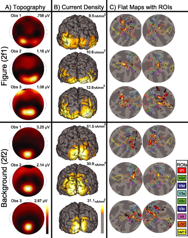
Scalp topography, CCD, and flattened cortical maps with visual area ROIs. SSVEP responses at the second harmonic of the figure (6.0 Hz) and background regions (7.2 Hz) are shown for three observers. Figure responses are shown in the top three panels, and background responses are shown in the bottom three panels. Responses are displayed in separate columns as spline-interpolated scalp voltage topographies (A), cortically constrained current density (B), and CCD projected onto flattened representations of the left and right hemispheres with visual area ROIs (C). Individual map maxima are indicated above the color scale. A, Figure responses show a lateral distribution over occipital sensors in all three participants. In contrast, background responses are focused tightly over midline occipital sensors. Background responses are two to three times larger than figure responses. B, Figure-related CCD distributions extended medially from first tier areas across the ventral surface of all three observers' cortices. Background-related current density was focused mostly on the occipital pole and extended along the dorsal midline. C, To assist in visualizing the CCD maps, we show flattened perspectives of each observer's left and right hemispheres in the far right columns. Visual area outlines are illustrated on each flat map, with the color corresponding to the legend on the right. Figure-related responses in all hemispheres are localized within the LOC ROI, whereas background-related responses are distributed across the V1, V2, and V3 ROIs.

The second column, Figure 3B, shows the CCD estimates of the second harmonics on the individual observer's cortical surfaces. These cortices are shown from a posterior view and with the current density thresholded at one-third the maximum. In each observer the figure region activity extends laterally from the occipital pole. In contrast, the background responses are maximal medially, with activity extending dorsally rather than laterally.

The third and fourth columns of Figure 3C show the current density estimates projected onto flat map representations of the left and right hemispheres. These flattened views are centered on the LOC and are presented along with that observer's retinotopically and functionally defined visual areas (V1, V2v, V2d, V3v, V3d, V3a, V4, LOC, and hMT+). In these flattened maps it can be seen that figure responses for all three observers are largest in the LOC, whereas background responses are distributed maximally over first tier visual areas (V1, V2, and V3). Similar response patterns were observed in the remaining participants.

Grand average response distributions

To summarize the differences in response distributions between the figure and background regions across all participants, we computed the second harmonic grand averages over all participants for each cue type (Fig. 4A–D) and the two attention conditions (Fig. 4E,F). In each row of Figure 4 a single frame of the stimulus is shown to the left of the average two-dimensional topography and three views of the CCD. Scale bars are provided, and the response maximum for each map is indicated.

As seen in the individual observers, the figure responses (left) are lateralized over the occipital cortex, whereas the background responses (right) are focused over the occipital midline. Importantly, the response distributions are similar for each cue type for both the figure and background.

To test the significance of sensor map differences between second harmonic responses to the figure and background regions and for each cue type, we performed a MANOVA on seven sensor locations corresponding approximately to Oz, P7, and P8 in the International 10-20 System. These sensors are illustrated with the filled symbols overlaid on the two-dimensional maps in Figure 4A. For sensor space MANOVA we designate this three-level factor by the term “channel.” The two-level factor “region” accounts for differences in harmonic response amplitudes to the figure and background regions of the stimulus. The four-level factor “cue” represents the three different form segmentation cues (orientation, phase, and temporal frequency) as well as a single level for either the harmonic of the figure-only or the full field background alone.

In the frequency sensor domain there was a significant effect of stimulus region (F_(1,8) = 13.252; p = 0.007) caused by larger amplitudes driven by the background. Furthermore, the responses on the midline (Oz) were larger than the lateral ones (F_(2,7) = 34.721; p < 0.001), but this effect was more pronounced for the background responses; the figure responses, in contrast, were distributed more laterally, generating a highly significant interaction between stimulus region and channel (F_(2,7) = 11.786; p = 0.006). This topographic distinction between figure and background responses was cue-invariant (F_(6,3) = 5.252; p = 0.101), although when region and channel were considered independently, they both varied weakly with cue (F_(3,6) = 6.101 and p = 0.030; F_(6,3) = 15.933 and p = 0.022, respectively). When collapsed over the other factors, there was an overall effect of cue (F_(3,6) = 37.962; p < 0.001) caused by the differences in magnitude for each cue type.

Attentional controls

Although attending to a stimulus is known to enhance the neural response to that stimulus (Reynolds and Chelazzi, 2004), scene segmentation mostly has been found to be a preattentive process in both human (Kastner et al., 2000; Schira et al., 2004) and monkey (Marcus and Van Essen, 2002). Nonetheless, it is possible that attention is drawn especially to figures and not background regions, and it is conceivable that the differences between region responses in the main experiment could be attributed to differences in attention. To assess the relative dependence of figure and background responses on attention, we compared the topographic distributions for the orientation-defined form stimulus recorded under three levels of task relevance: passive fixation, directed attention, and divided attention. Five observers who participated in the main experiment were recorded in a second session.

As in the main experiment there was a main effect of region (F_(1,4) = 11.529; p = 0.027) and channel (F_(2,3) = 11.281; p = 0.04) and a significant interaction between these two factors (F_(2,3) = 11.914; p = 0.037). However, attention did not interact significantly with either of these factors, nor did it influence the interaction between region and channel, indicating that the topographic specificity of figure and background processing was not attention-dependent.

Response magnitude profiles across visual areas

As noted in the discussion of Figure 2, the total response to either the figure or background region is composed of a series of harmonics, with the second harmonic being dominant. To capture as much activity of each stimulus region as possible, we pooled the amplitudes at each harmonic according to Equation 2 to produce a single magnitude estimate for each region in each visual area ROI.

Prominent figure region responses are present in the LOC ROI for the figure-only, orientation-defined form, and phase-defined form stimulus conditions, whereas the background region activity is maximal in first tier areas. This differential distribution of activity for the two regions is shown as magnitude profiles across the nine ROIs for nine participants in Figure 5A. The data are shown for the figure region on the left and the background region on the right. They are grouped by stimulus condition, with a single frame of that stimulus presented below to indicate visually the stimulus that was presented. All values were normalized to the observer's V1 ROI magnitude before averaging as a means to reduce observer variance caused by idiosyncratic amplitude differences. The V1 ROI absolute magnitudes used for normalization are indicated at the top of each histogram for reference. The error bars show the SEM across observer and hemispheres calculated according to Equation 2.

Figure 5.

Group average visual area response magnitudes and time courses. Figure-related (left) and background-related (right) responses are shown as the normalized magnitudes (A) and waveforms (B). Responses are grouped by stimulus condition, with one stimulus frame included in the center row for reference. Response magnitudes are displayed separately for each visual area (V1, red; V2, green; V3, blue; V3a, cyan; V4 magenta; MT+, yellow; LOC, orange). Error bars indicate 1 ± SEM. A, V1 normalized responses to the figure were maximal in the LOC ROI, whereas responses to the background were maximal in V2d and V3d ROIs. B, Average time courses for the Tier 1 ROI (dashed) and LOC ROI (solid) are plotted over one cycle of the figure and background stimulus cycles. The figure-related response in the Tier 1 ROI leads the larger response in the LOC ROI by ∼40 ms for the figure-only, orientation-defined form, and phase-defined form. Tier 1 and LOC also can be disassociated in the background response in which Tier 1 leads LOC and is of greater magnitude, although this difference is minimal in the full field condition, where there is no figure region.

The responses in the LOC ROI to the figure region are larger than those in the V1 ROI for the figure-only (2.65:1), orientation-defined form (2.8:1), and phase-defined form (2.05:1), whereas the background region produces more activity in the V1 ROI relative to the LOC ROI for each of these stimuli: figure-only (1:0.88), orientation-defined form (1:0.52), and phase-defined form (1:0.53). The responses from the LOC ROI thus are specialized for the figure region of these displays. The temporally defined figures, in contrast, evoked similar magnitudes in the V1 and LOC ROIs (1.07:1). These stimuli lack oriented texture elements extending away from the border of the figure and background regions and are segmentable only on the basis of differences in temporal frequency.

As described in Materials and Methods, the LOC ROI was defined in two ways, functionally and geometrically, for different observers. To establish that the preferential figure responses did not depend on the method of LOC ROI definition, we compared figure and background responses, using both definitions in the four observers who had functional localizers. Response magnitudes for the figure (geometric, 6.0; functional, 6.38) and background (geometric, 10; functional, 11.43) were similar with both methods of ROI definition and did not differ statistically.

The response magnitudes for both figure and background regions are smaller relative to V1 in ventral ROIs as compared with dorsal ones in the V2, V3 ROIs and in the V4 versus V3a ROIs. The dorsal/ventral distinction in V1/2/3 is correlated with lower and upper field projections and not dorsal and ventral pathway differences that might distinguish V3a and V4. It is a common observation in the visually evoked potential (VEP) literature that responses are larger to lower field stimuli than upper field ones (Michael and Halliday, 1971; Fortune and Hood, 2003), and our results appear to reflect this bias. It currently is not known whether this represents purely geometric factors or whether there are genuine processing differences between the upper and lower visual field. Given this, we may have underestimated the extent of activation in the V2v, V3v, and V4 ROIs.

To test region and cue differences across ROIs, we used a MANOVA design similar to that used to test differences in the sensor maps. Preliminary analyses indicated that magnitudes in lower tier areas V1, V2, and V3 were highly correlated, and we therefore collapsed the data across these regions into a single measurement, Tier 1. Individual observer magnitudes in Tier 1 were the coherent average over the right and left hemispheres of V1, V2d, V3d, V2v, and V3v. Activity in Tier 1 was contrasted with the coherent average of the right and left hemisphere LOC ROIs. The dependent variable was the ratio of figure region response magnitude divided by background response magnitude, in which total response amplitude is the root sum square of the first four plus the eighth harmonic amplitudes. The figure-to-background ratio (FBR) was larger in LOC (0.893) than in Tier 1 (0.414) (F_(1,9) = 15.308; p = 0.004).

The mean FBR ratio was 0.654 across cue types. Although FBR varied somewhat with cue type (figure-only, 0.611; orientation, 0.54; phase, 0.632; temporally defined form, 0.831), the main effect of cue was not quite significant (F_(3,7) = 3.768; p = 0.067), nor did it interact with Tier. As observed above in the frequency sensor domain, the source maps also showed a significant effect of stimulus region, reflected in the larger FBR in the LOC.

Time courses of figure activity in V1 and LOC

We visualized the temporal evolution of responses in the Tier 1 and LOC ROIs by selectively reconstructing their time series, using only the relevant harmonics (e.g., nf1 for the figure and nf2 for the background in which n is the harmonic number). As can be seen in Figure 5B, the waveform of the figure response in the Tier 1 ROI (dashed line) consists of alternating cycles of inward and outward current flow (positive and negative potential on the scalp). The figure responses are plotted on a 333 ms baseline corresponding to one period of the figure response (3 Hz). These waveforms were computed separately for each stimulus condition and each ROI by first averaging over vertices within an ROI for each observer and then across observers. The waveforms for both the Tier 1 and LOC ROIs were normalized to the RMS amplitude of each observer's Tier 1 CCD waveform before averaging across observers within the two ROIs. Background responses are plotted on the right of Figure 5B and are on the same baseline as the figure region responses. The full field waveforms extend to 333 ms, again corresponding to one period of the stimulus (3 Hz), but the other three conditions extend only to 277 ms, corresponding to one period of the 3.6 Hz background frequency.

The response waveforms for the figure region show two large peaks per stimulus cycle, consistent with the second harmonic being the dominant response component (Fig. 5B, left). Background responses show a similar structure, especially in Tier 1 (Fig. 5B, right). In absolute terms the background responses are much larger than the figure responses (see values at the top of each histogram) and are generated by a stimulus area that is approximately six times larger than the figure regions. Nonetheless, the background region evokes a relatively small response in the LOC ROI. Consistent with the profile of response magnitudes shown in Figure 5, peak-to-peak amplitudes show a double dissociation; figure region responses are largest in the LOC ROI, whereas background region responses are largest in the Tier 1 ROI.

Reliable differences in the time series between Tier 1 and LOC ROIs were present for the figure-only and orientation cues, both of which involved 90° orientation changes of the figure region. These differences are reflected in the dark bars above the time series, indicating significantly different time points between the two waveforms as identified by the permutation test. Background responses were reliably different for all cue types, being larger and faster in Tier 1 as compared with the LOC ROI.

Distribution of response maxima over time differ for figure and background regions

So that the temporal evolution of figure and background responses can be portrayed more intuitively, it is useful to visualize the full extent of activity on the cortical surface as it evolves in time. To do this, we used sensor space averaging of the filtered waveforms of all 13 observers (see Materials and Methods). Figure 6 shows five frames from one cycle of the figure response (top) and one cycle of the background response (bottom) from the orientation-defined form stimulus condition. These frames were selected to capture most adequately the qualitative differences in the response distributions over time. The first frame of each row occurs shortly after the current diminishes to zero (0 ms), and the relative delay of each successive frame is indicated below.

Figure 6.

Cortical distribution of figure and background responses over time. Average spatiotemporal maps derived from figure region (top) and background region (bottom) waveforms are presented as still frames on one observer's cortical surface for the orientation-defined form condition. Individual maps are thresholded at one-third of the maximum (gray) and are presented from a posterior perspective. The images are from time points during the respective stimulus periods that illustrate, qualitatively, the primary differences in cortical current distribution. The evolution of activity attributed to the figure progresses from first tier areas, located on the occipital pole, ventrally to lateral portions of the occipital cortex. Current density diminishes and then returns with the opposite polarity. In contrast, the background activity extends along the dorsomedial portion of the occipital cortex. The fact that these activity maps differ in their space/time distribution suggests that there are distinct cortical generators underlying figure and background processing. See the supplemental material for full animations (available at www.jneurosci.org).

As seen in the top five frames, the peak of activity associated with the figure region alternates between the first tier visual areas and the LOC. The direction of current flow alternates in the two halves of the response cycle in both posterior and lateral areas. In comparison, the spatial distribution of activity from the background region extends dorsally over time, rather than laterally. These patterns provide additional evidence that figure and background regions activate distinct sets of cortical areas. In addition, the figure-related activity in the LOC is preceded and followed by activity at the occipital pole, consistent with feedback from LOC to first tier areas, a topic that will be addressed additionally below.

A complete visualization of the response distributions over time requires a full animation on the cortical surface. These animations are provided for each of the cue types in the supplemental material (available at www.jneurosci.org). Animations of the spatiotemporal evolution of the figure responses show a periodic shifting of the activity maximum between medial and lateral occipital areas for each cue type. As apparent in the still frames presented in Figure 6, the background animations show a distinctly different pattern of activity that extends dorsally over medial occipital areas, rather than laterally.

Visual field topography

Because the LOC abuts the V1/V2/V3 foveal confluence region (Tootell and Hadjikhani, 2001), we were concerned that our figure region measurements may have mistaken activity in these first tier areas for LOC activity because we used small, centrally viewed figures. The fact that we observed different FBR magnitudes (Fig. 5A) and distinct time series in the Tier 1 and LOC ROIs (Fig. 5B) indicates that this is not the case, but we were interested in confirming this with an independent manipulation.

Although the V1/V2/V3 confluence region and the LOC border each other at low retinal eccentricities, peripheral locations are represented medially along the calcarine sulcus for V1/V2/V3, but they extend laterally, away from the center of the confluence region in the LOC (Tootell and Hadjikhani, 2001). If our figure region responses were generated exclusively by the V1/V2/V3 confluence region, the response topography should shift medially, and cortical sources also should shift when the stimuli are viewed in the periphery. If, on the other hand, the figure response indeed is generated in the LOC, the response topography should shift laterally or stay constant when the stimuli are shifted to the periphery, given the relatively weak retinotopy of the LOC. To test this, we used stimuli in which a 2° phase-defined form figure region was presented at different eccentricities in the visual field. This was accomplished by having observers fixate at each of five locations as depicted in Figure 7A.

We measured current density in the LOC ROI for both figure and background regions (Fig. 7B) and found that the figure region responses were contralateralized, as has been observed with fMRI (Tootell and Hadjikhani, 2001; Niemeier et al., 2005). Moreover, figure region responses (solid lines) in the LOC ROI of the contralateral hemisphere were always larger than the background responses (dashed lines). The responses from the LOC ROI of each hemisphere remain near-maximal within a hemifield, extending to peripheral fixations of 4°, with response magnitudes differing by only 6 and 3% for the left and right hemispheres, respectively. The background responses show little effect of figure location, which is not surprising, given the large extent of the background region. The weak dependence of response magnitude on eccentricity seen in the LOC ROI is more consistent with the retinotopy of the LOC (Niemeier et al., 2005) than that of V1/V2/V3. In addition, the figure response is not simply the response to foveal inputs, because the background region occupies this retinotopic space when fixation is directed away from the figure but is not sufficient to elicit a response comparable to that of the figure. Similarly, the background-alone condition also stimulates low eccentricities, but this is insufficient to elicit a preferential response in the LOC ROI (Fig. 5, full field).

Spatial scaling

It is well known that receptive field sizes increase at higher levels of the visual cortical hierarchy. Therefore, it is conceivable that larger receptive fields in the LOC may be recruited preferentially to distinguish the figure simply for display size reasons. If the figure were smaller, activation patterns related to figure and background might shift to reflect the relative spatial scaling of lower- and higher-level areas. To assess the influence of region size on figure response, we compared responses for the centrally presented 2° phase-defined form with the 5° phase-defined form stimulus of the main experiment.

Figure 8 shows the second harmonic figure and background scalp topographies and the ROI magnitude profiles for the 2° (left) and the 5° figures (right). Simple visual comparison reveals that the distributions and profiles are strikingly similar. The V1 ROI magnitudes indicated on each histogram demonstrate that, although the overall amplitude of the response does scale with the area of the region, the figure/background profiles do not. MANOVA performed on the ROI magnitudes with two levels of figure size reveals a main effect of region (F_(1,6) = 53.033; p < 0.001), a main effect of tier (F_(1,6) = 9.585; p = 0.021), and a significant interaction between region and tier (F_(1,6) = 12.413; p = 0.012). However, there is no effect of size, and size does not interact significantly with either of the other factors, nor does it influence the interaction between region and tier, indicating that the topographic specificity of figure and background processing is not size-dependent. Additional sensor space data from these five observers and four others, collected at figure sizes of 4, 8, and 16°, show a similar pattern; figure responses are always larger than background responses at lateral electrode sites.

Figure 8.

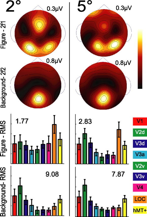
Test of size invariance. To evaluate the influence of region size on figure response, we compare region responses for the centrally presented 2° phase-defined form (left) with the 5° phase-defined form (right) stimulus of the main experiment. Similar response distributions and ROI magnitude profiles are present in the figure and background responses for each stimulus configuration. Error bars show the SEM across observers and hemispheres calculated according to Equation 2.

Discussion

A temporal tagging procedure has allowed us to analyze figure- and background-related activity separately during the simultaneous presence of both regions. Activity from both regions begins in low-level visual areas, but we find that the LOC preferentially represents the figure rather than the background region. Background-related activity, on the other hand, projects dorsally rather than laterally. Our analysis thus has provided the first direct evidence that figure and background regions activate distinct cortical networks. In previous EEG studies that used texture-defined forms (Caputo and Casco, 1999; Schubo et al., 2001; Romani et al., 2003; Casco et al., 2005), figure/background processing was studied by subtracting responses to segmented stimuli from those of uniform stimuli. This procedure effectively eliminates background-related activity and focuses the analysis on figure-related responses and nonlinear figure/background interactions. Analogous differencing procedures also have been used to study figure segmentation with fMRI (Grill-Spector et al., 1998; Kastner et al., 2000; Marcar et al., 2004; Schira et al., 2004; Scholte et al., 2006), and these studies suffer the same limitation. In single unit studies (Zipser et al., 1996; Rossi et al., 2001; Marcus and Van Essen, 2002) background and figure regions have always had the same time course, so it is unclear what fraction of the response is coming from the figure, the background, or their nonlinear interaction.

Cue invariance of the LOC

A necessary component of the perception of object shape is invariance with respect to changes in size, location, viewpoint, and surface properties. In our study the figure and background regions defined by differences in contrast, orientation, or alignment each produced a similar trajectory of activity through cortex. In each case the response to the figure region was relatively enhanced in the LOC ROI. The predominance of the figure region in the LOC also persisted over a range of retinal positions and figure sizes. The LOC thus shows a substantial degree of cue invariance as has been found with fMRI (Grill-Spector et al., 1998; Vuilleumier et al., 2002; Marcar et al., 2004).

Our figure regions activated an area of lateral cortex similar to that observed in human studies of illusory surfaces (Kanisza figures) and line drawings of common objects. Responses to illusory contour (IC) stimuli are maximal over lateral recording sites with both EEG (Murray et al., 2002, 2004; Pegna et al., 2002; Proverbio and Zani, 2002) and magnetoencephalography (Halgren et al., 2003). Murray and colleagues (2002) used dipole modeling to show that their IC activity colocalized with fMRI responses to the same stimuli at a location consistent with the LOC. Halgren et al. (2003) used a distributed inverse method to show that their IC activity was maximal in lateral cortical regions that were similarly active in an earlier fMRI study (Mendola et al., 1999). Other studies that used systematically degraded line drawings of simple objects found consistent activation of lateral occipital sites (Doniger et al., 2000), with a recent study showing colocalization of EEG and fMRI effects because of object completion in the LOC (Sehatpour et al., 2006). Synthetic figures depicting object silhouettes also produced BOLD activation in the LOC (Grill-Spector et al., 1998; Marcar et al., 2004). It thus appears that a wide range of object-like stimuli, in addition to images of recognizable objects, is capable of activating human LOC. Additional figure-related activity also was shown to extend beyond the LOC ROI in the surface-based animations, because was it present over frontal sites (Fig. 8). Similar activity extending temporally and into frontal cortex was observed by Halgren and colleagues (2003) in their study of illusory contour processing.

The temporally defined form stimulus deserves special consideration. First, the fact that this stimulus and related ones (Ramachandran and Rogers-Ramachandran, 1991; Fahle, 1993; Likova and Tyler, 2005) give rise to a perceptually segmented region is interesting in its own right. Segmentation of these stimuli must rely on the detection of purely temporal discontinuities, but how this is accomplished is unclear. The fact that the interior of the disk is filled in (e.g., seen as a disk and not a ring) implies either that the comparison of temporal asynchrony is made over a relatively large spatial extent or that the asynchrony is detected at the borders and the interior is filled in perceptually.

The ROI-based analysis showed preferential figure versus background activity for temporally defined forms in the LOC. We did not, however, see as clear a distinction between the time courses in the Tier 1 and LOC ROIs for this stimulus as for the others. The waveform of the response to the temporally defined form, as measured in the LOC ROI, is very similar to that for the other cue types, consistent with its being generated by the same underlying generators. On the other hand, the large differences in the spatial frequency content between the temporally defined form stimulus and the others may cause the response in the Tier 1 ROI to change its dynamics (slower) and/or the location of its generator. Either of these effects could make the waveforms in the Tier 1 and LOC ROIs more similar and harder to resolve.

In contrast to the ROI-based analysis, the animation of the temporally defined form response does show a periodic shifting of the activity maximum of the figure response between medial and lateral areas. Although this movement is less obvious than for the other cue types, it is still apparent. Moreover, there is a clear distinction in the activation sequence for the background and figure regions, as seen for the other cue types.

The role of attention in figure background processing

The pattern of figure background processing was mostly independent of whether the observers were fixating a mark in the center of the figure region, were discriminating threshold level changes in the figure shape, or were performing a difficult letter discrimination task. In each case the figure region responses were maximal in lateral cortex, whereas background activity was centered on the occipital pole. Previous EEG (Schubo et al., 2001) and fMRI studies (Kastner et al., 2000; Schira et al., 2004) each have found that differential responses to figure/ground displays occur under task conditions that rendered the observers unaware of the presence of segmentation. A recent combined MEG and fMRI study found a similar lack of an effect of attention on segmentation-related activity to an orientation-defined checkerboard presented in the periphery (Scholte et al., 2006). Knowledge of the presence of the figure/ground segmentation enhanced the texture segmentation evoked potential (Schubo et al., 2001), but it did not affect activation in V1, V2, V3, or V4 (Scholte et al., 2006). Figural enhancement also has been observed to occur outside the focus of attention in V1 and V2 (Marcus and Van Essen, 2002) but is not apparent under anesthesia (Lamme et al., 1998). Awareness and attention thus appear to play a modulatory, but not defining, role in figure/ground segmentation.

Selection of the figure region for processing in lateral cortex

The time course of the appearance and disappearance of a segmented figure in our displays is distinct from either the figure or background region time courses. Nonetheless, frequency-specific activity bearing the temporal signature of the figure region is emphasized specifically by the LOC, independent of the momentary interruptions of the appearance of a segmented figure. How is this region, and not the background, selected for routing to the LOC?

It has been shown that the LOC is selective for objects and spatial configurations similar to the ones we have used (Grill-Spector et al., 1998; Marcar et al., 2004). It is also known that the LOC shows persistent activation after the disappearance of a motion-defined object (Ferber et al., 2003, 2005; Large et al., 2005). Could object-selective neurons with long temporal integration times be responsible for our results? If this were the case, integration would have to occur over the intermittent, nonperiodic episodes of figure segmentation in our displays. Simple integration of these intermittent views of the figure would not, however, produce a response locked to the figure frequency tag.

Our results are more consistent with a feedback-driven process in which information from higher-level cortical areas is fed back to first tier visual areas as a means of selecting, or enhancing, figure region activity as an input to the LOC. There are several computational models that use feedback for region selection (Lee et al., 1998; Roelfsema et al., 2002; Thielscher and Neumann, 2003; Murray et al., 2004). These models differ in detail but include a higher-level stage that generates what is, in effect, a spatially weighted gating function that selects lower-level inputs for additional processing.

The apparent cycling of figure-related responses between the LOC and V1 ROIs, visible in the animations, is suggestive of, but by itself does not prove, the presence of feedback processing. Conclusive evidence for feedback processing in our system would entail a demonstration that changes in LOC activity drive changes in the first tier ROIs. The high-temporal resolution of the EEG lends itself to this sort of analysis, and several frequency domain methods for assessing functional connectivity have been developed (Schelter et al., 2006) and could applied to this problem.

In summary, source estimates from frequency-tagged EEG recordings have shown that the figure region of simple figure/ground displays preferentially activates regions of lateral occipital cortex that previously have been associated with object level processing. Responses to the background region project dorsally, rather than laterally, from the first tier visual areas. Responses in lateral cortical are mostly invariant with respect to the surface features used to define the figures, suggesting that the activity we have observed arises at a level of representation in which the low-level features of the retinal image have been abstracted. Whether these representations are primarily of surfaces or of borders awaits additional research. We expect that an analysis of the nonlinear figure/ground interaction terms may help to determine the relative contribution of border and surface cues at different levels of the object-processing hierarchy.

References

- Bevington PR, Robinson DK. New York: McGraw-Hill; 1992. Data reduction and error analysis for the physical sciences. [Google Scholar]
- Blair RC, Karniski W. An alternative method for significance testing of waveform difference potentials. Psychophysiology. 1993;30:518–524. doi: 10.1111/j.1469-8986.1993.tb02075.x. [DOI] [PubMed] [Google Scholar]
- Brewer AA, Liu J, Wade AR, Wandell BA. Visual field maps and stimulus selectivity in human ventral occipital cortex. Nat Neurosci. 2005;8:1102–1109. doi: 10.1038/nn1507. [DOI] [PubMed] [Google Scholar]
- Caputo G, Casco C. A visual evoked potential correlate of global figure-ground segmentation. Vision Res. 1999;39:1597–1610. doi: 10.1016/s0042-6989(98)00270-3. [DOI] [PubMed] [Google Scholar]
- Casco C, Grieco A, Campana G, Corvino MP, Caputo G. Attention modulates psychophysical and electrophysiological response to visual texture segmentation in humans. Vision Res. 2005;45:2384–2396. doi: 10.1016/j.visres.2005.02.022. [DOI] [PubMed] [Google Scholar]
- DeYoe EA, Carman GJ, Bandettini P, Glickman S, Wieser J, Cox R, Miller D, Neitz J. Mapping striate and extrastriate visual areas in human cerebral cortex. Proc Natl Acad Sci USA. 1996;93:2382–2386. doi: 10.1073/pnas.93.6.2382. [DOI] [PMC free article] [PubMed] [Google Scholar]
- Doniger GM, Foxe JJ, Murray MM, Higgins BA, Snodgrass JG, Schroeder CE, Javitt DC. Activation timecourse of ventral visual stream object-recognition areas: high density electrical mapping of perceptual closure processes. J Cogn Neurosci. 2000;12:615–621. doi: 10.1162/089892900562372. [DOI] [PubMed] [Google Scholar]
- Fahle M. Figure-ground discrimination from temporal information. Proc Biol Sci; 1993. pp. 199–203. [DOI] [PubMed] [Google Scholar]
- Ferber S, Humphrey GK, Vilis T. The lateral occipital complex subserves the perceptual persistence of motion-defined groupings. Cereb Cortex. 2003;13:716–721. doi: 10.1093/cercor/13.7.716. [DOI] [PubMed] [Google Scholar]
- Ferber S, Humphrey GK, Vilis T. Segregation and persistence of form in the lateral occipital complex. Neuropsychologia. 2005;43:41–51. doi: 10.1016/j.neuropsychologia.2004.06.020. [DOI] [PubMed] [Google Scholar]
- Fortune B, Hood D. Conventional pattern-reversal VEPs are not equivalent to summed multifocal VEPs. Invest Ophthalmol Vis Sci. 2003;44:1364–1375. doi: 10.1167/iovs.02-0441. [DOI] [PubMed] [Google Scholar]
- Geesaman BJ, Andersen RA. The analysis of complex motion patterns by form/cue invariant MSTd neurons. J Neurosci. 1996;16:4716–4732. doi: 10.1523/JNEUROSCI.16-15-04716.1996. [DOI] [PMC free article] [PubMed] [Google Scholar]
- Grill-Spector K, Kushnir T, Edelman S, Itzchak Y, Malach R. Cue-invariant activation in object-related areas of the human occipital lobe. Neuron. 1998;21:191–202. doi: 10.1016/s0896-6273(00)80526-7. [DOI] [PubMed] [Google Scholar]
- Halgren E, Mendola J, Chong CD, Dale AM. Cortical activation to illusory shapes as measured with magnetoencephalography. NeuroImage. 2003;18:1001–1009. doi: 10.1016/s1053-8119(03)00045-4. [DOI] [PubMed] [Google Scholar]
- Hamalainen MS, Ilmoniemi RJ. Interpreting magnetic fields of the brain: minimum norm estimates. Med Biol Eng Comput. 1994;32:35–42. doi: 10.1007/BF02512476. [DOI] [PubMed] [Google Scholar]
- Huk AC, Dougherty RF, Heeger DJ. Retinotopy and functional subdivision of human areas MT and MST. J Neurosci. 2002;22:7195–7205. doi: 10.1523/JNEUROSCI.22-16-07195.2002. [DOI] [PMC free article] [PubMed] [Google Scholar]
- Kastner S, De Weerd P, Ungerleider LG. Texture segregation in the human visual cortex: a functional MRI study. J Neurophysiol. 2000;83:2453–2457. doi: 10.1152/jn.2000.83.4.2453. [DOI] [PubMed] [Google Scholar]
- Keselman HJ, Algina J, Kowalchuk RK. The analysis of repeated measures designs: a review. Br J Math Stat Psychol. 2001;54:1–20. doi: 10.1348/000711001159357. [DOI] [PubMed] [Google Scholar]
- Kourtzi Z, Kanwisher N. Cortical regions involved in perceiving object shape. J Neurosci. 2000;20:3310–3318. doi: 10.1523/JNEUROSCI.20-09-03310.2000. [DOI] [PMC free article] [PubMed] [Google Scholar]
- Lamme VA, Zipser K, Spekreijse H. Figure-ground activity in primary visual cortex is suppressed by anesthesia. Proc Natl Acad Sci USA. 1998;95:3263–3268. doi: 10.1073/pnas.95.6.3263. [DOI] [PMC free article] [PubMed] [Google Scholar]
- Lamme VA, Rodriguez-Rodriguez V, Spekreijse H. Separate processing dynamics for texture elements, boundaries, and surfaces in primary visual cortex of the macaque monkey. Cereb Cortex. 1999;9:406–413. doi: 10.1093/cercor/9.4.406. [DOI] [PubMed] [Google Scholar]
- Large ME, Aldcroft A, Vilis T. Perceptual continuity and the emergence of perceptual persistence in the ventral visual pathway. J Neurophysiol. 2005;93:3453–3462. doi: 10.1152/jn.00934.2004. [DOI] [PubMed] [Google Scholar]
- Lee TS, Nguyen M. Dynamics of subjective contour formation in the early visual cortex. Proc Natl Acad Sci USA. 2001;98:1907–1911. doi: 10.1073/pnas.031579998. [DOI] [PMC free article] [PubMed] [Google Scholar]
- Lee TS, Mumford D, Romero R, Lamme VA. The role of the primary visual cortex in higher level vision. Vision Res. 1998;38:2429–2454. doi: 10.1016/s0042-6989(97)00464-1. [DOI] [PubMed] [Google Scholar]
- Lee TS, Yang CF, Romero RD, Mumford D. Neural activity in early visual cortex reflects behavioral experience and higher-order perceptual saliency. Nat Neurosci. 2002;5:589–597. doi: 10.1038/nn0602-860. [DOI] [PubMed] [Google Scholar]
- Leventhal AG, Wang Y, Schmolesky MT, Zhou Y. Neural correlates of boundary perception. Vis Neurosci. 1998;15:1107–1118. doi: 10.1017/s0952523898156110. [DOI] [PubMed] [Google Scholar]
- Likova LT, Tyler CW. Transient-based image segmentation: top-down surround suppression in human V1. Proc Int Soc Opt Eng; 2005. pp. 248–257. [Google Scholar]
- Lin FH, Witzel T, Ahlfors SP, Stufflebeam SM, Belliveau JW, Hamalainen MS. Assessing and improving the spatial accuracy in MEG source localization by depth-weighted minimum-norm estimates. NeuroImage. 2006;31:160–171. doi: 10.1016/j.neuroimage.2005.11.054. [DOI] [PubMed] [Google Scholar]
- Malach R, Reppas JB, Benson RR, Kwong KK, Jiang H, Kennedy WA, Ledden PJ, Brady TJ, Rosen BR, Tootell RB. Object-related activity revealed by functional magnetic resonance imaging in human occipital cortex. Proc Natl Acad Sci USA. 1995;92:8135–8139. doi: 10.1073/pnas.92.18.8135. [DOI] [PMC free article] [PubMed] [Google Scholar]
- Marcar VL, Raiguel SE, Xiao D, Orban GA. Processing of kinetically defined boundaries in areas V1 and V2 of the macaque monkey. J Neurophysiol. 2000;84:2786–2798. doi: 10.1152/jn.2000.84.6.2786. [DOI] [PubMed] [Google Scholar]
- Marcar VL, Loenneker T, Straessle A, Jaggy S, Kucian K, Martin E. An fMRI study of the cerebral macro network involved in “cue invariant” form perception and how it is influenced by stimulus complexity. NeuroImage. 2004;23:947–955. doi: 10.1016/j.neuroimage.2004.05.028. [DOI] [PubMed] [Google Scholar]
- Marcus DS, Van Essen DC. Scene segmentation and attention in primate cortical areas V1 and V2. J Neurophysiol. 2002;88:2648–2658. doi: 10.1152/jn.00916.2001. [DOI] [PubMed] [Google Scholar]
- Mendola JD, Dale AM, Fischl B, Liu AK, Tootell RB. The representation of illusory and real contours in human cortical visual areas revealed by functional magnetic resonance imaging. J Neurosci. 1999;19:8560–8572. doi: 10.1523/JNEUROSCI.19-19-08560.1999. [DOI] [PMC free article] [PubMed] [Google Scholar]
- Michael WF, Halliday AM. Differences between the occipital distribution of upper and lower field pattern-evoked responses in man. Brain Res. 1971;32:311–324. doi: 10.1016/0006-8993(71)90327-1. [DOI] [PubMed] [Google Scholar]
- Murray MM, Wylie GR, Higgins BA, Javitt DC, Schroeder CE, Foxe JJ. The spatiotemporal dynamics of illusory contour processing: combined high-density electrical mapping, source analysis, and functional magnetic resonance imaging. J Neurosci. 2002;22:5055–5073. doi: 10.1523/JNEUROSCI.22-12-05055.2002. [DOI] [PMC free article] [PubMed] [Google Scholar]
- Murray MM, Foxe DM, Javitt DC, Foxe JJ. Setting boundaries: brain dynamics of modal and amodal illusory shape completion in humans. J Neurosci. 2004;24:6898–6903. doi: 10.1523/JNEUROSCI.1996-04.2004. [DOI] [PMC free article] [PubMed] [Google Scholar]
- Murray SO, Schrater P, Kersten D. Perceptual grouping and the interactions between visual cortical areas. Neural Netw. 2004;17:695–705. doi: 10.1016/j.neunet.2004.03.010. [DOI] [PubMed] [Google Scholar]
- Niemeier M, Goltz HC, Kuchinad A, Tweed DB, Vilis T. A contralateral preference in the lateral occipital area: sensory and attentional mechanisms. Cereb Cortex. 2005;15:325–331. doi: 10.1093/cercor/bhh134. [DOI] [PubMed] [Google Scholar]
- Pegna AJ, Khateb A, Murray MM, Landis T, Michel CM. Neural processing of illusory and real contours revealed by high-density ERP mapping. NeuroReport. 2002;13:965–968. doi: 10.1097/00001756-200205240-00013. [DOI] [PubMed] [Google Scholar]
- Proverbio AM, Zani A. Electrophysiological indexes of illusory contours perception in humans. Neuropsychologia. 2002;40:479–491. doi: 10.1016/s0028-3932(01)00135-x. [DOI] [PubMed] [Google Scholar]
- Ramachandran VS, Rogers-Ramachandran DC. Phantom contours: a new class of visual patterns that selectively activates the magnocellular pathway in man. Bull Psychonomic Soc. 1991;29:391–394. [Google Scholar]
- Ramsden BM, Hung CP, Roe AW. Real and illusory contour processing in area V1 of the primate: a cortical balancing act. Cereb Cortex. 2001;11:648–665. doi: 10.1093/cercor/11.7.648. [DOI] [PubMed] [Google Scholar]
- Reynolds JH, Chelazzi L. Attentional modulation of visual processing. Annu Rev Neurosci. 2004;27:611–647. doi: 10.1146/annurev.neuro.26.041002.131039. [DOI] [PubMed] [Google Scholar]
- Roelfsema PR, Lamme VA, Spekreijse H, Bosch H. Figure-ground segregation in a recurrent network architecture. J Cogn Neurosci. 2002;14:525–537. doi: 10.1162/08989290260045756. [DOI] [PubMed] [Google Scholar]
- Romani A, Callieco R, Tavazzi E, Cosi V. The effects of collinearity and orientation on texture visual evoked potentials. Clin Neurophysiol. 2003;114:1021–1026. doi: 10.1016/s1388-2457(03)00075-0. [DOI] [PubMed] [Google Scholar]
- Rossi AF, Desimone R, Ungerleider LG. Contextual modulation in primary visual cortex of macaques. J Neurosci. 2001;21:1698–1709. doi: 10.1523/JNEUROSCI.21-05-01698.2001. [DOI] [PMC free article] [PubMed] [Google Scholar]
- Sary G, Vogels R, Orban GA. Cue-invariant shape selectivity of macaque inferior temporal neurons. Science. 1993;260:995–997. doi: 10.1126/science.8493538. [DOI] [PubMed] [Google Scholar]
- Schelter B, Winterhalder M, Eichler M, Peifer M, Hellwig B, Guschlbauer B, Lucking CH, Dahlhaus R, Timmer J. Testing for directed influences among neural signals using partial directed coherence. J Neurosci Methods. 2006;152:210–219. doi: 10.1016/j.jneumeth.2005.09.001. [DOI] [PubMed] [Google Scholar]
- Schira MM, Fahle M, Donner TH, Kraft A, Brandt SA. Differential contribution of early visual areas to the perceptual process of contour processing. J Neurophysiol. 2004;91:1716–1721. doi: 10.1152/jn.00380.2003. [DOI] [PubMed] [Google Scholar]
- Scholte HS, Witteveen SC, Spekreijse H, Lamme VA. The influence of inattention on the neural correlates of scene segmentation. Brain Res. 2006;1076:106–115. doi: 10.1016/j.brainres.2005.10.051. [DOI] [PubMed] [Google Scholar]
- Schubo A, Meinecke C, Schroger E. Automaticity and attention: investigating automatic processing in texture segmentation with event-related brain potentials. Brain Res Cogn Brain Res. 2001;11:341–361. doi: 10.1016/s0926-6410(01)00008-8. [DOI] [PubMed] [Google Scholar]
- Sehatpour P, Molholm S, Javitt DC, Foxe JJ. Spatiotemporal dynamics of human object recognition processing: an integrated high-density electrical mapping and functional imaging study of “closure” processes. NeuroImage. 2006;29:605–618. doi: 10.1016/j.neuroimage.2005.07.049. [DOI] [PubMed] [Google Scholar]
- Thielscher A, Neumann H. Neural mechanisms of cortico-cortical interaction in texture boundary detection: a modeling approach. Neuroscience. 2003;122:921–939. doi: 10.1016/j.neuroscience.2003.08.050. [DOI] [PubMed] [Google Scholar]
- Tootell RB, Hadjikhani N. Where is “dorsal V4” in human visual cortex? Retinotopic, topographic, and functional evidence. Cereb Cortex. 2001;11:298–311. doi: 10.1093/cercor/11.4.298. [DOI] [PubMed] [Google Scholar]
- Tyler CW, Likova LT, Kontsevich LL, Wade AR. The specificity of cortical region KO to depth structure. NeuroImage. 2006;30:228–238. doi: 10.1016/j.neuroimage.2005.09.067. [DOI] [PubMed] [Google Scholar]
- Victor JD, Mast J. A new statistic for steady-state evoked potentials. Electroencephalogr Clin Neurophysiol. 1991;78:378–388. doi: 10.1016/0013-4694(91)90099-p. [DOI] [PubMed] [Google Scholar]
- Vuilleumier P, Henson RN, Driver J, Dolan RJ. Multiple levels of visual object constancy revealed by event-related fMRI of repetition priming. Nat Neurosci. 2002;5:491–499. doi: 10.1038/nn839. [DOI] [PubMed] [Google Scholar]
- Wade AR, Brewer AA, Rieger JW, Wandell BA. Functional measurements of human ventral occipital cortex: retinotopy and colour. Philos Trans R Soc Lond B Biol Sci. 2002;357:963–973. doi: 10.1098/rstb.2002.1108. [DOI] [PMC free article] [PubMed] [Google Scholar]
- Zhan CA, Baker CL., Jr Boundary cue invariance in cortical orientation maps. Cereb Cortex. 2006;16:896–906. doi: 10.1093/cercor/bhj033. [DOI] [PubMed] [Google Scholar]
- Zipser K, Lamme VA, Schiller PH. Contextual modulation in primary visual cortex. J Neurosci. 1996;16:7376–7389. doi: 10.1523/JNEUROSCI.16-22-07376.1996. [DOI] [PMC free article] [PubMed] [Google Scholar]