

Abstract
The diffusion of proteins in the cell membrane is investigated using computer simulations of a two-dimensional model. The membrane is assumed to be divided into compartments, with adjacent compartments separated by a barrier of stationary obstacles. Each compartment contains traps represented by stationary attractive disks. Depending on their size, these traps are intended to model either smaller compartments or binding sites. The simulations are intended to model the double-compartment model, which has been used to interpret single molecule experiments in normal rat kidney cells, where five regimes of transport are observed. The simulations show, however, that five regimes are observed only when there is a large separation between the sizes of the traps and large compartments, casting doubt on the double compartment model for the membrane. The diffusive behavior is sensitive to the concentration and size of traps and the strength of the barrier between compartments suggesting that the diffusion of proteins can be effectively used to characterize the structure of the membrane.
Introduction
The lateral diffusion of proteins in plasma membranes is important in many physiological processes and has been studied extensively using experiment and computer simulation. In addition to the intrinsic interest in the diffusive behavior of proteins, these studies also provide insight into the structure of the membrane itself, which is very heterogeneous (1–3). For example, the diffusion of proteins in cell membranes is orders-of-magnitude slower than in artificial membranes (4–6), and this difference cannot be accounted for solely by the presence of a physiological amount of obstacles that hinder the diffusion. The relation between the structure of plasma membranes and protein diffusion is not considered well understood despite extensive research (2,4–7). Recently, Kusumi et al. (2), Ritchie et al. (8), and Suzuki et al. (9) proposed a new structural model for the membrane that relies on the division of the cell membrane into compartments. In this work, we present a computer simulation study of a simple model that includes compartments and quantify their effect on the diffusion of proteins.
Kusumi et al. (2) and Ritchie et al. (8) proposed a fence and picket model for the structure of the plasma membrane. In this model, the membrane is compartmentalized into corrals with junctional complexes of integral membrane proteins acting as pickets and components, e.g., spectrin filaments, of the underlying cytoskeleton acting as fences that create a barrier to protein diffusion. At short timescales, the protein displays Brownian motion, with a diffusion constant comparable to artificial membranes that they interpreted as diffusion within a compartment. On intermediate timescales, the trajectories show a hopping motion of the proteins that they interpreted as a hopping over the barriers between compartments. On large timescales, when a large enough number of hops have been sampled, diffusive motion is recovered, although with a much smaller diffusion coefficient than that at short times. On timescales longer than that for diffusion within a compartment, but smaller than when normal diffusion is recovered at long times, the proteins display anomalous diffusion where the mean-squared displacement 〈R2(t)〉 scales with time t as 〈R2(t)〉 ∼ tα with α < 1 (α = 1 for normal diffusion). The three time regimes of protein diffusion have been observed in many experiments (8,10–15).
A strict compartmentalization is not necessary to explain these experiments. In fact, the diffusion of lipid molecules in the outer leaflet also shows similar diffusion behavior for which one cannot invoke direct hopping over the cytoskeleton (16). Computer simulations of hard disks in two-dimensional space with randomly spaced obstacles (which are also hard disks) also show these three regimes (7,17). The compartments in this case are pockets of space without obstacles and are connected to other pockets via channels. Narrow channels act as entropic barriers over which proteins hop between pockets. Recently, Auth and Gov reported a simulation study on the effect of a flexible network of long-chain proteins on the protein diffusion for the red blood cell (18) and found that the stretching of cytoskeletons and anchor proteins could influence the protein diffusion significantly.
Recently, Suzuki et al. (9) studied the diffusion of a G-protein-coupled receptor in the normal rat kidney cell (NRK) membranes. From their analysis of high-resolution single molecule trajectories, they found five distinct regimes (instead of three) for protein diffusion (Fig. 1). They suggested a model where the plasma membrane of the NRK cell is doubly compartmentalized with small compartments (230 nm) within larger compartments (750 nm) (16,19).
Figure 1.
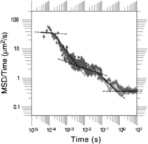
Sketch (reproduced from Suzuki et al. (9)) of the time-dependent diffusion coefficient, D(t), as a function of time in the double compartment model showing the five different regimes of diffusion.
As Suzuki et al. (9) point out in their article, this is only a qualitative model, and careful calculations are necessary to see whether the model reproduces the experimental results. Nevertheless, the model raises very significant questions. One would expect five regimes only if there was a timescale over which the protein had sampled many small compartments but had not yet felt the confinement due to the larger compartments, i.e., when there is a large separation of timescales between diffusion in small and large compartments. This does not seem likely in a system where the size ratio of small compartments to large compartments is only 1/3. Other mechanisms, such as the binding of proteins to domains, must be also tested to confirm the validity of the double compartmentalization model. Other questions might be posed. What is the most significant factor that determines the exponent α in each regime? How does the interaction between proteins and each of these compartments affect the protein dynamics? Does the size ratio of small compartments to big compartments change the behavior in the protein diffusion? We address these issues in this work using computer simulations.
In this work, we study a simple model of the membrane where it is divided into compartments separated by repulsive barriers (see Fig. 2). A protein is confined within a compartment and has to overcome the repulsive interaction to escape to a neighboring compartment. Within each compartment, there are many traps that are attractive to the proteins. Depending on their size (which we vary), these traps may be viewed as small compartments (if the traps are larger than proteins) or as protein binding sites (if the traps are much smaller than large compartments). Monte Carlo simulations for protein diffusion show five regimes (instead of three) for certain values of parameters, and this allows us to investigate the effect of molecular interactions and the concentration and size of small compartments on the protein diffusion. Our simulations suggest that the experimental results can also be explained using a single compartment model if there is some binding of the protein to the membrane, and that the strict double compartmentalization might not be necessary.
Figure 2.
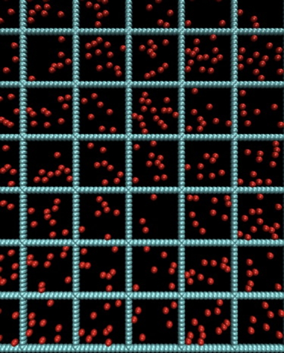
Model for the membrane. The barriers are represented by a sequence of blue (fence) disks of diameter σF = 1.5σ with a distance σ (≡ 1) between adjacent disks. The red disks are traps of diameter σT, which is varied from 0.5 to 3.5σ. A protein experiences a repulsive interaction when it is within a distance of σF/2 from a fence disk and an attractive interaction when it is within a distance of σT/2 from a trap disk.
The rest of the article is organized as follows. The simulation method is described in the next section, and results are presented and discussed in the section after that, followed by Conclusions.
Models and Simulations
We use a coarse-grained description of proteins and membrane components to investigate the diffusive behavior of proteins on timescales of over eight orders of magnitude. The plasma membrane is modeled as a two-dimensional space with two types (F for fence and T for trap) of immobile disks. The diameter, σF of a fence disk is 1.5 σ, where σ (the unit of length in this article) is the distance between the centers of adjacent fence disks. The fence disks are placed in a grid with equally spaced vertical and horizontal lines (Fig. 2). The large compartments are therefore squares bounded by the fence disks, with a distance between two adjacent parallel lines of grids of 12σ; this sets 12σ ≈ 1–3 μm. Periodic boundary conditions are used in both directions with a periodic simulation box size, L = 84σ. The diameter of the trap disks, σT, is varied from 0.5 to 3.5. The mobile protein is modeled as a point particle. Initial conditions are generated by first creating a grid of fences and then inserting the traps at randomly chosen positions, provided they do not overlap with other fence and trap disks. If an attempted insertion of a trap overlaps with an existing trap or fence, a new position is attempted for the insertion. For σT = 3.5, it is difficult to insert traps in this fashion and for that one case the traps are placed at square lattice points such that they do not overlap each other. Once the disks are inserted, they are frozen in space. Properties are averaged for each configuration, and then averaged over five different independent configurations of the membrane. Error bars are reported as the standard deviation about the mean of these five independent calculations.
We investigate several area fractions of the traps, defined by ϕT = πNTσT2/4L2 where NT is the number of traps. We report results for ϕT = 0.0125–0.6, which corresponds to ∼5–33 traps depending on σT.
A protein is modeled as a point particle that interacts with the fence disks with a repulsive interaction, VF(r), and with the traps with an attractive interaction, VT(r). We use a square well interaction, i.e.,
| (1) |
| (2) |
where r is the distance between the protein and the center of the disk and β ≡ 1/kBT, where kB is Boltzmann's constant and T is temperature. All energy values are in units of kBT. Unless otherwise noted, the height of the repulsive wall, Vrep is fixed at 6. The strength of an attractive well, Vatt, is varied from 5 to 9.
In our simplified model, Vatt and σT are taken to be the same for all traps in a given system. Unless otherwise noted, the variability in σT and Vatt is ignored. This is, of course, a simplification because cell membranes are very heterogeneous, and a more sophisticated model would have different values of Vatt and σT for different traps. The noise in the time-dependent diffusion coefficient, in the third regime of Fig. 1, could be precisely because of this variability. Such variability in Vatt and σT introduces additional quenched disorder into the system and additional computational complications. It requires an averaging over all realizations of the different parameters, i.e., many more starting points and much longer trajectories. We perform additional simulations with variability introduced in σT and Vatt by using distribution functions that are simple, yet still ensure the largest variability. We use
| (3) |
and
| (4) |
In our simulations, a = 0.75 and σ0 = 2 are used so the average value (σ0) of σT is 2.0. We find that the time-dependent diffusion coefficients are quite sensitive to b, and the simulations can fit the experiments only for b = 7.5.
Monte Carlo (MC) simulations are performed using a standard Metropolis algorithm in a canonical ensemble. In our MC simulations, only the protein moves via random displacement with a maximum displacement of 0.1σ. For a given configuration of traps up to 10 billion random walks are conducted. The number of attempted moves is taken to be the unit of time, t, in this work. The mean-squared displacement, 〈R2(t)〉 and the time-dependent diffusion coefficient, D(t) are calculated using
| (5) |
| (6) |
where r(t) is the position of the fluid particle at time, t, and 〈…〉 denotes the ensemble average over trajectories and configurations of the traps.
Results and Discussion
The traps can be viewed as either small compartments or protein binding sites. If the traps are large compared to the proteins (but smaller than the large compartments), then the protein is confined to some extent within the disks (because there is an energetic penalty to leaving the trap region). If, on the other hand, the traps are much smaller than large compartments, then they can be viewed as protein binding sites. Changing the size of the traps allows us to investigate both these scenarios.
If the traps are approximately the estimated size of small compartments (in experiments on NRK cells), then the simulation results for D(t) do not display the experimentally observed behavior. Fig. 3 depicts D(t) as a function of time for ϕT = 0.6, Vatt =7, and σT = 3.5. In experiments on NRK cells, the small compartments are 210–260 nm and the large compartments are 710–750 nm. Since the size of the large compartments is 12σ, the size of the small compartment comparable to the estimated size in experiments should be between 3.36σ and 4.4σ. Fig. 3 shows that only three diffusive regimes are observed for σT = 3.5σ in contrast to the five regimes seen in experiment.
Figure 3.
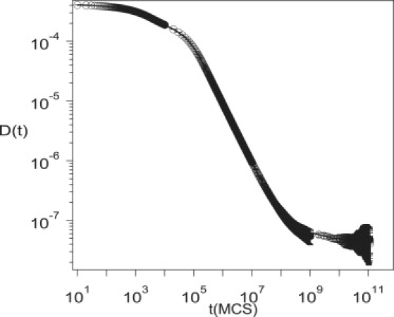
Simulation results for the time-dependent diffusion coefficient as a function of time for ϕT = 0.6, Vatt = 5, Vrep = 6, and σT = 3.5, which corresponds to the double-compartment model. Only three regimes are observed in this case, in contrast to the five regimes in Fig. 2.
In our model, a protein can take a random walk with a maximum step of 0.1. Therefore, when σT > 3.4, there is a chance that a channel of free passage should exist and a protein can hop between small traps without feeling the energy barriers. Therefore, we carried out additional simulations with σT = 0.34, 0.344, 0.345, and 0.346 to investigate the effect of the free passage. Five regimes in the diffusion were observed even with a channel of free passage, suggesting that the disappearance of the five regimes for σT = 3.5 should not be due simply to the channel of free passage. Instead, the values of α for the second and the third regimes for σT ≥ 3.4 were quite big compared to experiments, and the five regimes in the diffusion thus become obscure with an increase in σT.
If the size of the traps becomes smaller, however, the five diffusive regimes are clearly captured in our simulations. Fig. 4, a and b, depicts the mean-squared displacement, 〈R2(t)〉 and time-dependent diffusion coefficient, D(t), respectively, for ϕT = 0.05, Vatt = 5, Vrep = 6, and σT = 1. Simulations with three different time resolutions are used to obtain the entire curve. The diffusion coefficient changes drastically with time by more than two orders of magnitude in our simulations. At short (I) and long (V) timescales, the protein exhibits Brownian motion with α ≈ 1 even though diffusion coefficients are very different. For intermediate times, the diffusion coefficient decreases with time and three regimes (II, III, and IV) can be discerned from one another by different values of α.
Figure 4.
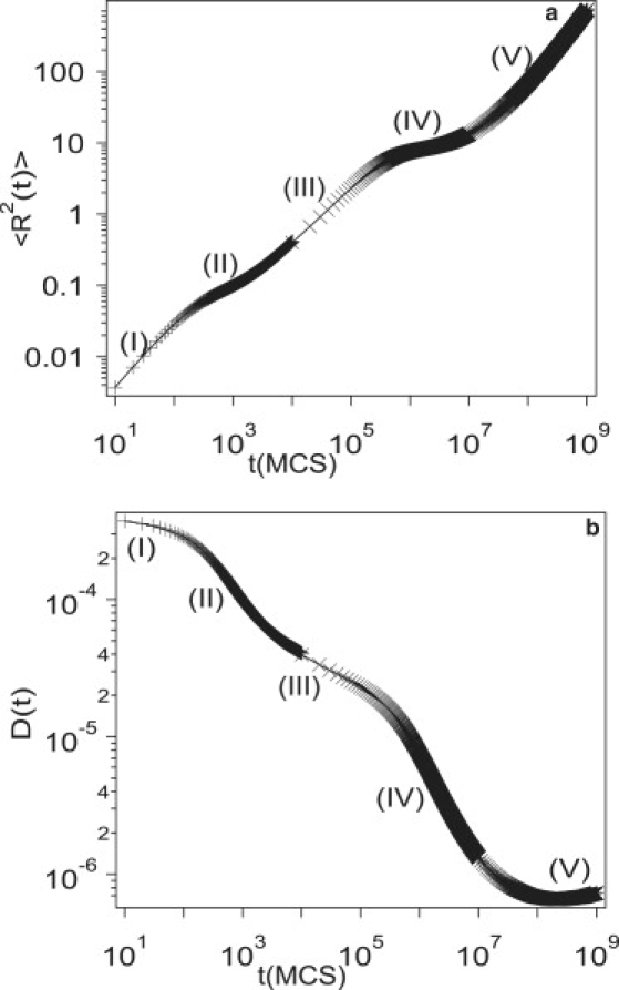
Simulation results for (a) mean-squared displacements, 〈R2(t)〉 and (b) the time-dependent diffusion coefficient, D(t), as a function of time, for ϕT = 0.05, Vatt = 5, Vrep = 6, and σT = 1. Roman numbers indicate the five regimes of protein dynamics determined by time exponents of mean-squared displacements.
The five regimes are not observed if either of the traps or fences are removed. Fig. 5 depicts D(t) for three cases: 1), with both small and large compartments (circles); 2), with only small compartments (dashed line); and 3), with only large compartments (dashed-dotted-dotted line). If either the traps or the fences are present, D(t) starts out flat, decreases for intermediate times (due to anomalous diffusion), and then becomes flat for large times. In both of these cases, however, there are only three regimes (not five). With only small compartments, a protein can visit many small compartments after ∼1000 time-steps, and normal diffusive behavior is recovered for t = 103. With only big compartments, the diffusion coefficient at long times is larger than with both small and big compartments because there are no small compartments to temporarily trap the protein.
Figure 5.
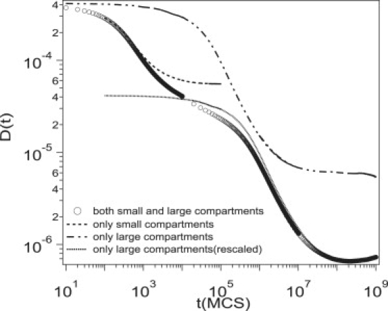
Simulation results for D(t) for three different cases: 1), with both small and large compartments (circles); 2), with only small compartments (dashed); and 3), with only large compartments (dashed-dotted-dotted). The time-dependent diffusion coefficients calculated with only large compartments is rescaled with Ns = 10. (dotted; see the text for details) For all cases, ϕT = 0.05, Vatt = 5, Vrep = 6, and σT = 1.
The simulations are consistent with the qualitative interpretation of the experiment regarding the five regimes. If only the small compartments are present, the simulations give the dashed line, which agrees with the simulations with both compartments at short times. If only the large compartments are present we obtain the dashed-dotted-dotted line, but we have to rescale the meaning of the time-step to compare to the simulations with both compartments. Let us assume that a protein obtains a mean-square displacement of R2 after a time Nst with both compartments, and the same displacement after a time t in the absence of the small compartments. Since R2 = 4DbothNst = 4Dlarget (where Dboth and Dlarge are the diffusion constants with both compartments and only large compartments), we can compare simulations with only large compartments to the simulations with both compartments by multiplying time by a factor of Ns and dividing the diffusion coefficient by a factor of Ns. The dotted curve is obtained from the dashed-dotted-dotted curve using a value of Ns = 10. The agreement between this curve and the curve obtained from simulations with both compartments suggests that regime IV arises from anomalous diffusion due to the hindrance of the large compartments.
The quantitative behavior of D(t) is sensitive to the concentration of traps and the strength of their interaction, but the qualitative behavior is similar for a wide range of parameters. Fig. 6 depicts D(t) for different concentrations of traps, ϕT (= 0.025, 0.05 and 0.1) for Vatt = 5, Vrep = 6, and σT = 1. For short times, the protein is confined within a single small compartment, and D(t) is insensitive to the concentration. In regime III, however, D(t) is smaller for larger concentrations because the attractive traps tend to decrease D(t) in this regime. The timescale over which D(t) enters regime IV, however, is not sensitive to concentration. It has been argued that the presence of attractive traps should not change the diffusion constant at long times when averaged over all initial positions. D(t) is insensitive to concentration in regime IV because here it is determined primarily by the features of the large compartments.
Figure 6.
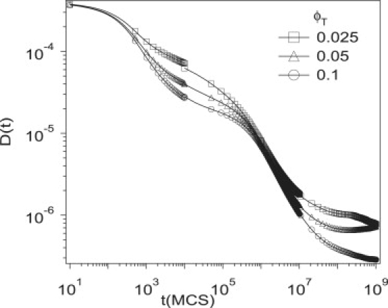
Simulation results for the time-dependent diffusion coefficient, D(t), for different concentrations of traps, ϕT = 0.025, 0.05, and 0.1, for Vatt = 5, Vrep = 6, and σT = 1.
The strength of the interaction with the traps (Vatt) significantly changes the timescales over which D(t) enters regimes III and IV. Fig. 7 depicts D(t) for Vatt = 5, 7, and 9 for ϕT = 0.05, Vrep = 6, and σT = 1. As Vatt increases, there are larger barriers for the protein to leave a trap and it takes longer for the protein to sample the space of traps. Therefore, D(t) does not plateau until longer times, resulting in a sharper decrease at short times.
Figure 7.
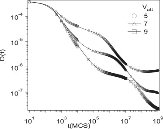
Simulation results for the time-dependent diffusion coefficient, D(t), for different interaction strengths of small compartments, Vatt = 5, 7, and 9 for ϕT = 0.05, Vrep = 6, and σT = 1. Different values of ϕT are used.
Fig. 8 depicts D(t) for different sizes of traps (σT = 0.5, 1, 2, and 3.5). In this figure, Vatt = 5 and Vrep = 6. The value of ϕT is adjusted such that the average number of traps in a large compartment are kept constant: ϕT = 0.0125, 0.05, and 0.2 for σT = 0.5, 1, and 2, respectively. When σT = 3.5, ϕT = 0.6 because it is the biggest possible value. As σT is increased, the time period of regime III decreases as does the exponent α in this regime. If σT is increased further, as in Fig. 3 the third regime disappears and we are left with three instead of five regimes.
Figure 8.
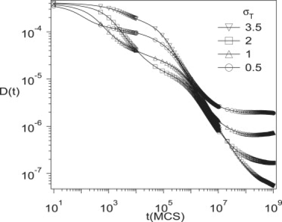
Simulation results for the time-dependent diffusion coefficient, D(t), for different sizes of traps, σT = 0.5, 1, 2, and 3.5 for Vatt = 5 and Vrep = 6. Values of ϕT are adjusted for a large compartment to contain approximately the same number of traps, i.e., ϕT = 0.0125, 0.05, and 0.2 for σT = 0.5, 1, and 2, respectively. Note that ϕT = 0.6 for σT = 3.5, because traps should be located at lattices and ϕT = 0.6 is the only possible number for such a case.
A direct comparison of the model with experimental data is complicated because it is not possible to independently determine the values of the model parameters. Therefore, we resort to fitting these parameters to the experiments. The first issue is that of matching the timescale and length-scale of the simulations to experiments. As pointed out by Suzuki et al. (9) determining the size of the large compartments is subtle, but the value is expected to be ∼1–2 μm, which suggests σ ≈ 83–167 nm. By (roughly) matching the position of the plateau, we rescale the time axis so that 1 MC step is 0.25 μs. We still have four undetermined parameters, namely, σT, ϕT, Vatt, and Vrep, which are adjusted to find the best fit to the experiments. A best fit is obtained with σT = 2σ, ϕT = 0.14, Vrep = 3.75, and Vatt = 5. Note that this set might not be unique; i.e., other parameter sets might result in a comparably good agreement with experiments. Fig. 9 depicts the comparison of simulations to experiments by changing σT (Fig. 9 a) and Vrep (Fig. 9 b), respectively. In this comparison, the size of large compartments is fixed. In both cases, Vatt = 5 and ϕT = 0.14; Vrep = 3.75 in Fig. 9 a and σT = 2 in Fig. 9 b. Changing Vrep affects only the long-time behavior, and changing σT affects only the short time behavior, and this gives us confidence that these parameters are not correlated. From the fit, we can determine that the size of the traps is ∼2σ, i.e., the trap size is in the range 166–334 nm. This suggests that the size ratio of small compartments to large compartments should be much smaller than suggested by Suzuki et al. (9).
Figure 9.
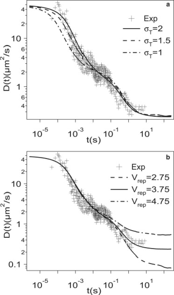
Comparison of simulation results for D(t) to experiments (9) for different values of (a) σT and (b) Vrep. Note that Vatt = 5 and ϕT = 0.14 (for both a and b); and that Vrep = 3.75 (a), σT = 2 (b).
It is interesting to investigate the effect of heterogeneity in trap sizes and strengths. In the simulations, this can be achieved by choosing the parameters σT and Vatt from a probability distribution function. The motivation for investigating a variability in these parameters is the qualitative observation that there is considerable scatter in the experimental results in the third regime (see Fig. 1) and it is of interest to ascertain the origin of this behavior. Fig. 10 shows time-dependent coefficients for four cases: (Fig. 10 a) with no variability in σT or Vatt; (Fig. 10 b) with variability in only σT; (Fig. 10 c) with variability in both σT and Vatt; and (Fig. 10 d) the same as case c, but for a longer trajectory.
Figure 10.
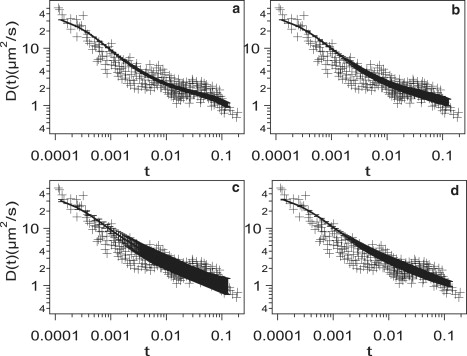
Comparison of simulation results for D(t) to experiments (9) with a variability in σT and Vatt, values of which are chosen from a flat probability distribution, for ϕT = 0.14 and Vrep = 3.7. (a) No variability in σT or Vatt; (b) variability in σT but not in Vatt; (c) variability in both σT and Vatt; and (d) same as for panel c, but for trajectories 10-times as long. The values of the parameters (see text for definition) are a = 0.75, σ0 = 2, and b = 7.5.
The trajectories are 50 million steps long for Fig. 10, a–c, and 500 million steps long for Fig. 10 d. The variability in σT does not change D(t) significantly (comparing panels a and b in Fig. 10). This is because the potential energy of the protein is constant for steps within small compartments and the protein feels the potential difference only when it crosses the boundaries of small compartments. In Fig. 10 c, the probability that the protein escapes small compartments is different and this affects the dynamics significantly. The simulations can fit the data only for b = 7.5 (Eq. 4). More interestingly, the statistical uncertainties become large when a variability in Vatt is incorporated, requiring long trajectories. This suggests that the experimental scatter in time-dependent diffusion coefficients in the third regime could be attributed to the variability in Vatt.
Conclusions
We study the diffusion of proteins in compartmentalized membranes using simulations. The model consists of small compartments nested within larger compartments. In the simulations, the mean-squared displacement and time-dependent diffusion coefficient of a protein in plasma membranes are investigated over a time-range of eight orders of magnitude.
The simulations show five different regimes in protein dynamics, but only if there is a sufficient separation in the length-scales of the small and large compartments. This requires a much larger ratio of sizes (between large and small compartments) than estimated from experiments. This suggests that either the ratio of the size of the small compartments to the large compartments is somewhat smaller (1/6) than inferred in the experiments (1/3) or that a different mechanism (such as binding of protein to small domains) is responsible for the five diffusive regimes seen in single molecule experiments. Therefore, more experimental and theoretical studies are requested to test the validity of the compartment model for the NRK membrane structure.
The value of the time-dependent diffusion coefficient in different regimes as well as the exponent α are sensitive to the model parameters (although the qualitative behavior only requires a separation of size scales between small and large compartments). This suggests that our model can be used to extract information regarding the structure of the membrane from measurements of the time-dependent diffusion coefficient. A good fit to experimental data is obtained for σT = 2, ϕT = 0.14, Vrep = 3.75, and Vatt = 5. The important information extracted from this fit is that the size of the small compartments is roughly 340 nm, if the large compartments are 2 μm. In other words, to fit the data we need ∼36 traps (or small compartments) within each large compartment. This estimate for the size ratio of the small compartments to the large compartments is much smaller than suggested by experiment (9) where each large compartment is estimated to have only a few small compartments. So what could these small compartments be? One possibility is the existence of lipid domains (rafts) to which the proteins segregate. Recently, Andrew et al. have observed the actin cables near the cell membranes that hinder the protein diffusion (20). They suggested that these actin cables should build a dynamic labyrinth of micron-sized actin barriers instead of a static mesh network. The dynamic labyrinth could act as a large compartment for a protein diffusion. A more definitive answer would require more experimental information regarding the structure of the plasma membrane.
Recently, Kenkre et al. (21) proposed an analytical theory to describe the protein diffusion in compartments. The analytical theory allows one to calculate the time-dependent diffusion coefficients and extract the compartment size from the experimental data. However, the theory is limited to relatively simple systems with no double compartments. Although the theory can be easily extended to our model, this extension is not trivial. The combination of our simulation studies and such analytical theories would provide us with a deeper understanding of protein diffusion in cell membranes and tools to extract essential information on the cell membranes such as Vatt and σT. A further study will be required to extend the theory and conduct more simulations.
The cell membrane is very heterogeneous, and protein diffusion is expected to be influenced by many other factors not considered in our study. For example, proteins could bind to other proteins or segregate to lipid domains (18). If proteins aggregate, their self-diffusion coefficient will become much smaller because the diffusion coefficient is inversely proportional to the protein size. Incorporation of these effects would be an interesting future direction of this work.
Acknowledgments
This material is based upon work supported by the National Science Foundation under grant No. CHE-0717569.
This work was supported by the Korea Research Foundation, funded by the Korean Government (Ministry of Education and Human Resources Development grant No. KRF-2008-331-C00141). This work was also supported by Sogang University (research grant No. 20071116).
References
- 1.Glaser M. Lipid domains in biological-membranes. Curr. Opin. Struct. Biol. 1993;3:475–481. [Google Scholar]
- 2.Kusumi A., Nakada C., Ritchie K., Murase K., Suzuki K. Paradigm shift of the plasma membrane concept from the two-dimensional continuum fluid to the partitioned fluid: high-speed single-molecule tracking of membrane molecules. Annu. Rev. Biophys. Biomol. Struct. 2005;34:351–354. doi: 10.1146/annurev.biophys.34.040204.144637. [DOI] [PubMed] [Google Scholar]
- 3.Engelman D.M. Membranes are more mosaic than fluid. Nature. 2005;438:578–580. doi: 10.1038/nature04394. [DOI] [PubMed] [Google Scholar]
- 4.Saxton M.J., Jacobson K. Single-particle tracking: applications to membrane dynamics. Annu. Rev. Biophys. Biomol. Struct. 1997;26:373–399. doi: 10.1146/annurev.biophys.26.1.373. [DOI] [PubMed] [Google Scholar]
- 5.Vrljic M., Nishimura S.Y., Brasselet S., Moerner W.E., McConnell H.M. Translational diffusion of individual class II MHC membrane proteins in cells. Biophys. J. 2002;83:2681–2692. doi: 10.1016/S0006-3495(02)75277-6. [DOI] [PMC free article] [PubMed] [Google Scholar]
- 6.Deverall M.A., Gindl E., Sinner E.K., Besir H., Ruehe J. Membrane lateral mobility obstructed by polymer-tethered lipids studied at the single molecule level. Biophys. J. 2005;88:1875–1886. doi: 10.1529/biophysj.104.050559. [DOI] [PMC free article] [PubMed] [Google Scholar]
- 7.Sung B.J., Yethiraj A. Lateral diffusion and percolation in membranes. Phys. Rev. Lett. 2006;96:228103. doi: 10.1103/PhysRevLett.96.228103. [DOI] [PubMed] [Google Scholar]
- 8.Ritchie K., Lino R., Fujiwara T., Murase K., Kusumi A. The fence and picket structure of the plasma membrane of live cells as revealed by single molecule techniques (Review) Mol. Membr. Biol. 2003;20:13–18. doi: 10.1080/0968768021000055698. [DOI] [PubMed] [Google Scholar]
- 9.Suzuki K., Ritchie K., Kajikawa E., Fujiwara T., Kusumi A. Rapid hop diffusion of a G-protein-coupled receptor in the plasma membrane as revealed by single-molecule techniques. Biophys. J. 2005;88:3659–3680. doi: 10.1529/biophysj.104.048538. [DOI] [PMC free article] [PubMed] [Google Scholar]
- 10.Ghosh R.N., Webb W.W. Automated detection and tracking of individual and clustered cell-surface low-density-lipoprotein receptor molecules. Biophys. J. 1994;66:1301–1318. doi: 10.1016/S0006-3495(94)80939-7. [DOI] [PMC free article] [PubMed] [Google Scholar]
- 11.Selle C., Rückerl F., Martin D.S., Forstner M.B., Käs J.A. Measurement of diffusion in Langmuir monolayers by single-particle tracking. Phys. Chem. Chem. Phys. 2004;6:5535–5542. [Google Scholar]
- 12.Feder T.J., Brust-Mascher I., Slattery J.P., Baird B., Webb W.W. Constrained diffusion or immobile fraction on cell surfaces: a new interpretation. Biophys. J. 1996;70:2767–2773. doi: 10.1016/S0006-3495(96)79846-6. [DOI] [PMC free article] [PubMed] [Google Scholar]
- 13.Periasamy N., Verkman A.S. Analysis of fluorophore diffusion by continuous distributions of diffusion coefficients: application to photobleaching measurements of multicomponent and anomalous diffusion. Biophys. J. 1998;75:557–567. doi: 10.1016/S0006-3495(98)77545-9. [DOI] [PMC free article] [PubMed] [Google Scholar]
- 14.Saxton M.J. Anomalous subdiffusion in fluorescence photobleaching recovery: a Monte Carlo study. Biophys. J. 2001;81:2226–2240. doi: 10.1016/S0006-3495(01)75870-5. [DOI] [PMC free article] [PubMed] [Google Scholar]
- 15.Jin S., Verkman A.S. Single particle tracking of complex diffusion in membranes: simulation and detection of barrier, raft, and interaction phenomena. J. Phys. Chem. B. 2007;111:3625–3632. doi: 10.1021/jp067187m. [DOI] [PubMed] [Google Scholar]
- 16.Fujiwara T., Ritchie K., Murakoshi H., Jacobson K., Kusumi A. Phospholipids undergo hop diffusion in compartmentalized cell membrane. J. Cell Biol. 2002;157:1071–1081. doi: 10.1083/jcb.200202050. [DOI] [PMC free article] [PubMed] [Google Scholar]
- 17.Sung B.J., Yethiraj A. Lateral diffusion of proteins in the plasma membrane: spatial tessellation and percolation theory. J. Phys. Chem. B. 2008;112:143–149. doi: 10.1021/jp0772068. [DOI] [PubMed] [Google Scholar]
- 18.Auth T., Gov N.S. Diffusion in a fluid membranes with a flexible cortical cytoskeleton. Biophys. J. 2009;96:818–830. doi: 10.1016/j.bpj.2008.10.038. [DOI] [PMC free article] [PubMed] [Google Scholar]
- 19.Murase K., Fujiwara T., Uemura Y., Suzuki R., Iino H. Ultrafine membrane compartments for molecular diffusion as revealed by single molecule techniques. Biophys. J. 2004;86:4075–4093. doi: 10.1529/biophysj.103.035717. [DOI] [PMC free article] [PubMed] [Google Scholar]
- 20.Andrews N.L., Lidke K.A., Pfeiffer J.R., Burns A.R., Wilson B.S. Actin restricts FcɛRI diffusion and facilitates antigen-induced receptor immobilization. Nat. Cell Biol. 2008;10:955. doi: 10.1038/ncb1755. [DOI] [PMC free article] [PubMed] [Google Scholar]
- 21.Kenkre V.M., Giuggioli L., Kalay Z. Molecular motion in cell membranes: analytic study of fence-hindered random walks. Phys. Rev. E Stat. Nonlin. Soft Matter Phys. 2008;77:051907. doi: 10.1103/PhysRevE.77.051907. [DOI] [PubMed] [Google Scholar]