Structural Information, Resolution, and Noise in High-Resolution Atomic Force Microscopy Topographs

Abstract

AFM has developed into a powerful tool in structural biology, providing topographs of proteins under close-to-native conditions and featuring an outstanding signal/noise ratio. However, the imaging mechanism exhibits particularities: fast and slow scan axis represent two independent image acquisition axes. Additionally, unknown tip geometry and tip-sample interaction render the contrast transfer function nondefinable. Hence, the interpretation of AFM topographs remained difficult. How can noise and distortions present in AFM images be quantified? How does the number of molecule topographs merged influence the structural information provided by averages? What is the resolution of topographs? Here, we find that in high-resolution AFM topographs, many molecule images are only slightly disturbed by noise, distortions, and tip-sample interactions. To identify these high-quality particles, we propose a selection criterion based on the internal symmetry of the imaged protein. We introduce a novel feature-based resolution analysis and show that AFM topographs of different proteins contain structural information beginning at different resolution thresholds: 10 Å (AqpZ), 12 Å (AQP0), 13 Å (AQP2), and 20 Å (light-harvesting-complex-2). Importantly, we highlight that the best single-molecule images are more accurate molecular representations than ensemble averages, because averaging downsizes the z-dimension and “blurs” structural details.

Introduction

AFM in structural biology

AFM (1) has developed into a powerful tool in membrane research (2). Topographs at submolecular resolution can be acquired under close-to-native conditions in buffer and under ambient pressure and temperature on 2D-crystallized (3) or densely packed (4) membrane proteins, and most recently on single-component (5) and multicomponent native membranes (6,7). These images represent a strong basis for structural models of multiple membrane protein complexes working together (8,9). Such AFM images are generally termed “high-resolution AFM topographs”.

High resolution in structural biology

The meaning of “high resolution” in structural biology depends on the technique considered. In NMR studies, a well-defined structure determines the position of atoms with an RMSD of ∼0.5 Å (F. Cordier, Institut Pasteur de Paris, France, personal communication, 2008 (10)). In x-ray crystallography of 3D crystals, the term high-resolution is applied to a resolution better than 2 Å or, more stringently, when atomic resolution (∼1.2 Å) is achieved (D. Picot, Institut de Biologie Physico-Chimique, Paris, France, personal communication, 2008) (11). In EM, the term is again applied differently and is furthermore attributed to distinct nominal resolutions depending on the subfield: in EM crystallography of 2D crystals, structures determined to a resolution better than ∼3.5 Å are considered to be at high resolution (12). High resolution in single particle analysis is achieved at a resolution better than 10 Å (13), except for the analysis of highly symmetrical particles, i.e., viruses, where 4 Å were achieved (14). Finally, in biological AFM studies, when topographical features smaller than the protein molecule itself were observed, the term high-resolution AFM was applied.

The term high resolution is hence purely qualitative, technique dependent, and changing with time. However, it is noteworthy that the transposition of structural information among NMR, x-ray, and EM data is fairly well assessed: NMR and x-ray structures are successfully rendered to and docked into lower-resolution EM envelopes (13), because EM densities have been used to phase x-ray diffraction patterns (15). AFM data represent an exception to this: so far, AFM topographic information is used to complement information from other techniques (8,9,16), the resolution issue is not well addressed, and comparison with data sets acquired by other techniques of identical objects evokes considerable discrepancies in terms of features seen at distinct resolutions.

Discrepancies between resolution and structure assessment in EM and AFM

It has been reported that some AFM topographs had lateral resolution better than 5 Å (16). Unfortunately, although there was a scientific basis for such resolution assignments, there are obvious discrepancies between the structural features expected to be seen at this resolution (i.e., amino acids) and what is actually visible in such topographs. The discrepancies are particularly problematic when the AFM analysis is compared directly with EM data of the same sample: the AFM images, although having higher resolution than the EM images (as determined by DPR (17), the FRC (18), the SSNR (19,20), or the observation of the outermost diffraction spots in calculated power spectra of highly ordered 2D crystals (21)), often display fewer structural features than the latter. As an illustration, we discuss three examples: Fisrt, bR: the best AFM topographs on purple membrane, native 2D crystals of bR were reported to resolve the bR surface to better than 5 Å resolution (16,22). In these topographs, three features corresponding to the cytoplasmic loops are visible. In contrast, EM projection maps of the same sample at 7 Å resolution reveal seven density features corresponding to the seven transmembrae helices (23,24). Second, AqpZ: the AFM topography of the extracellular surface of AqpZ was determined to 7 Å resolution and revealed three features per monomer (25). In contrast, the EM projection at 8 Å resolution revealed approximately six density peaks (26). Third, AQP0: the AFM topography of the extracellular surface of AQP0 was determined to 6.1 Å resolution. This topography revealed two protrusions per AQP0 monomer (21). The accompanying EM projection map of the same 2D crystals determined to 6.9 Å resolution revealed approximately nine densities per AQP0 monomer (21).

For these three examples, the structural information provided by AFM is poor compared with the EM data, and with what is expected from the resolution limit reported. Today, atomic structures of bR (27,28), AqpZ (29), and AQP0 (30,31) are available and allow comparison with the lower-resolution EM and AFM data. The above examples illustrate the need to further analyze in detail the signal, resolution, and significance of structural features reported in AFM topographs. This knowledge will bring credibility to the AFM technique, advance the understanding of AFM imaging, and allow the information contributed by AFM to be integrated with data from other techniques applied in structural biology.

In this work, we analyze AFM topographs. First, we study noise and distortions, finding that many molecule images in high-resolution AFM topographs are only slightly disturbed. To identify these images, we discuss cross-correlation searches and propose an image-selection criterion based on the IS of the protein studied. Next, we propose a novel feature-based resolution assessment method that can be applied to ensemble averages but also to single molecules. We conclude that significant structural information can be found in high-resolution AFM topograph between 10 Å and 20 Å resolution depending on the sample studied, in agreement with structural analysis performed by other imaging techniques. Finally, we show that AFM is a real single-molecule analysis technique, because best single molecules are better structural representations than ensemble averages.

Materials and Methods

AFM

The AFM (1) was operated in contact mode at ambient temperature and pressure. Imaging was performed with a commercial Nanoscope-E AFM (Veeco, Santa Barbara, CA) equipped with a 150-μm scanner (J-scanner) and oxide-sharpened Si₃N₄ cantilevers (length 100 μm; k = 0.09 N/m; Olympus Ltd., Tokyo, Japan). For imaging, minimal loading forces of ∼100 pN were applied, at scan frequencies of 4–7 Hz, using optimized feedback parameters. For more details see (21).

Data analysis

All image treatment and analysis of AFM topographs were performed using a JAVA-based image processing routine integrated in the ImageJ program (32). All AFM topographs had an image size of 512 × 512 pixels and were 8-bit gray-scale formatted, resulting in a total range of 256 gray values for the total z-range.

To quantify the total noise present in AFM topographs, several images containing different amounts of noise were computed by superpositioning a noise-free artificial AqpZ 2D crystal (in silico assemblage of the unit cell, 113 unit cells in total) with 10%, 20%, 30%, 40%, 50%, 60%, 70%, 80%, or 90% of Gaussian white noise (mean 117 gray values; SD 36 gray values; average gray value change on pixel: 1, 2, 4, 9, 17, 30, 49, 70, or 94 gray values, respectively). Furthermore, a noise-free image was superpositioned by a Gaussian noise gradient ranging from 0% to 80%. To identify single particles in these images, cross-correlation maps with a noise-free reference image (i.e., unit cell of the artificial AqpZ 2D crystal) were calculated, and the resulting CCV was used as selection criterion for each particle:

$$\text{CCV}=\frac{\sum _i(p_{\left(i\right)}-\overline{p})\times (q_{\left(i\right)}-\overline{q})}{\sqrt{\sum _i{(p_{\left(i\right)}-\overline{p})}^2\times \sum _i{(q_{\left(i\right)}-\overline{q})}^2}}\text{.}$$ (1)

The difference of the pixel value and the mean gray value of the image is calculated for each pixel (i) in the reference (p) and the raw data (q) images, normalized, and integrated, resulting in a CCV at each image position that will be equal to 1 in case of identity of images compared.

These in silico measurements of the resemblance (i.e., CCV) of a noise-free reference compared with images containing defined amounts of noise were used for a calibration graph. With this standard, we estimated the average gray value deviation of raw data AFM topographs from an average. The reference images used to analyze CCV of raw data AFM topographs were ensemble averages of all molecules present in the image after translational and rotational alignment.

Averaging of aligned molecule images is addition and normalization of pixels in the image matrix following:

$$\text{Ave}=1/N\sum \left(x_{ij}\right),$$ (2)

where N is the number of molecules averaged, and x_ij stands for the gray value of pixel i in particle image j.

Concomitantly, a SD map is calculated as follows.

$$\text{SD}=\sqrt{\raisebox{1ex}{$1$}\!\left/ \!\raisebox{-1ex}{$N-1$}\right.\sum {(x_{ij}-{\overline{x}}_j)}^2},$$ (3)

where N is the number of molecules, x_ij stands for the gray value of pixel i in molecule j and, ${\overline{x}}_j$ for the average gray value of pixel j.

We define the IS as the CCV between a molecule and itself after n-fold symmetrization. We define the ACV as the CCV between a molecule and itself after low-pass filtering.

Results and Discussion

Noise quantification in AFM topographs

Images are a superposition of signal and noise (19). The signal originates from the object, whereas the noise is apparatus contributed or image acquisition related. The quantity of these parameters and the manner in which they behave are technique specific, and knowledge of them is important for interpretation of data originating from a particular technique. In AFM topographs, we subdivide noise into noise and distortions. Noise is apparatus contributed and randomly distributed on the topographs. On the contrary, distortions are scanning related, only present in some regions of the topographs, and generally appear as scan lines. They mainly originate from different acquisition speeds of the different scan axes, “parachuting” of the AFM probe, or insufficient or excess force, to name a few reasons. In this section, we analyze the total amount of noise and distortions.

For this, we compared how well a noise-free reference finds molecules of its kind by calculating CCVs in 1), images combining noise-free molecules and known amounts of noise, and in 2), an AFM topograph (Fig. 1).

Figure 1.

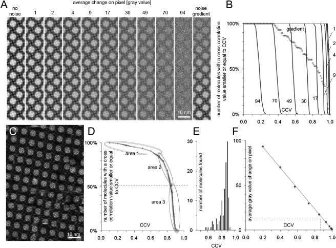
Total noise assessment in a high-resolution AFM topograph. (A) Superposition of different amounts of Gaussian noise to a noise-free artificial AqpZ 2D crystal. (B) Graph displaying the number of molecules found in the images shown in A as a function of the CCV used as selection criterion. (C) Raw data AFM topograph (extract of a larger image, full gray scale: 15 Å). (D) Graph displaying the number of molecules found in the image shown in C by several references (black to increasingly light gray lines: reference comprising all, 50%, 25% of the molecule images, 3, and 1 molecule image) as a function of CCV used as selection criterion. (E) Histogram showing the number of molecules found at a given CCV. (F) Calibration graph used to estimate the average change of gray values on a pixel after the addition of distinct amounts of noise in the images shown in A. The average pixel gray value deviation of the real AFM topograph is estimated to be 14 gray values (i.e., 1 Å) (dashed line).

We computed (see Materials and Methods) several images in which noise-free molecules were superpositioned by white Gaussian noise (Fig. 1 A, left 10 panels). Furthermore, we computed an image in which noise-free molecules are superpositioned by a Gaussian noise gradient (Fig. 1 A, right panel). Depending on the amount of added noise, graphs plotting the number of molecules found versus CCV (Fig. 1 B) display horizontal lines corresponding to 100% of molecules detected until a certain CCV threshold, above which no molecules were found. The graphs drop almost vertically, because all molecules within each artificial image were superposed by the same amount of noise and were therefore discriminated at approximately the same CCV (Fig. 1 B, solid lines). When a linear gradient of noise was added to an image, the number of molecules found as a function of the CCV decreased linearly (Fig. 1 B, crosses). These in silico measurements of the resemblance of a noise-free reference compared with images containing defined amounts of noise were used for a calibration graph. With this standard, we estimated the average gray value deviation of raw data AFM topographs from an average (Fig. 1 F).

Cross-correlation analyses of references with an AFM topograph (Fig. 1 C) are documented by graphs displaying the number of molecules found as function of the CCV (Fig. 1 D). In such a realistic case, the CCV graphs have three sections: the first part of the curve is approximately horizontal between a low CCV threshold of 0.1, where 100% of the molecules (127) were found, and a CCV of 0.6, where 90% were found. In other words, 10% of the molecules in the image were of low quality. In the second area in the graph, molecules with CCVs between 0.6 and 0.85 were discriminated. Another 40% of molecules cross-correlated between these values and hence still contained an increased amount of noise compared with the best ones identified in the third region (Fig. 1 D). In this third region, 50% of all molecules were found with CCVs of 0.85 to 0.92 (Fig. 1 E).

From this analysis, we draw three important conclusions. First, in the analyzed topograph, the rejection of 50% of the molecule images is favorable for structure analysis, and the remaining best 50% of molecules images are only minimally disturbed. Second, using the computational noise-gradient analysis as standard, we found that each pixel in the AFM topograph deviated on average by 14 gray values from a noise-free average (Fig. 1 F). Because gray values correspond to height information, this deviation corresponds to a height noise of 1 Å per pixel. Third, regardless of whether single-molecule or average images were used as a reference, the resulting curves were similar (see Fig. 1 D). Because best single molecules have a CCV of ∼0.9, they cross-correlated with other molecules in the image, as well as the ensemble averages.

IS as a molecule image selection criterion

As shown above, it is crucial to identify the molecule images with the highest quality. Here, we propose to use IS of n-fold symmetrical molecules as selection criterion. The IS is a direct measure of the image quality, because an oligomer of n times the biochemically identical unit is expected to have good n-fold symmetry. This is a key consideration for AFM, because topographs may reveal scan lines or directional deformation of molecules in the fast- and slow-scan axes and the imperfect adjustment of loading forces or feedback parameters. Analysis of the IS makes sense for a technique with a high SNR.

First, we analyzed how the IS of average images and SD maps depend on the quality and number of images merged (Fig. 2 A). The analysis of the IS of averages revealed that an average of all molecules is not most symmetrical (Fig. 2 B, right). In agreement with Fig. 1 D, it appeared that 50% of the molecules in the topograph had been significantly disturbed. Once these images were excluded from the average, the IS was 0.965. This high value indicates that the remaining good molecule images are basically free of distortions. The IS remained at this high level even when only the three best molecule images were averaged. The best single-molecule image still had a striking IS of 0.95 (Fig. 2 B, left), a strong argument for the quality of single-molecule images. SD maps reveal the structure in the image where pixel values deviate between molecules and have therefore been interpreted as documenting protein flexibility (33,34). As the SD maps emphasize the nonconstant structure factors in images, the IS of SD maps is lower than that of averages and decreases strongly as the number of molecule images merged is below 30 (Fig. 2 C, left). The IS of the SD maps increased to a maximum of 0.90 when between 30 (∼25%) and 90 molecules (∼75%) were merged, and dropped when all molecules were integrated (Fig. 2 C, right). We consider the IS to be a quality control of SD maps, because the movements of each of the subunits of the tetrameric AqpZ is thought to be equivalent and independent. AFM images contain noise and distortions. The noise is equally distributed on the four AqpZ subunits, and therefore the IS gets better when more molecules are merged. In contrast, scan-related distortions merged in averages and SD maps drop the IS, illustrating the ternary character of AFM images comprising signal, noise, and distortion.

Figure 2.

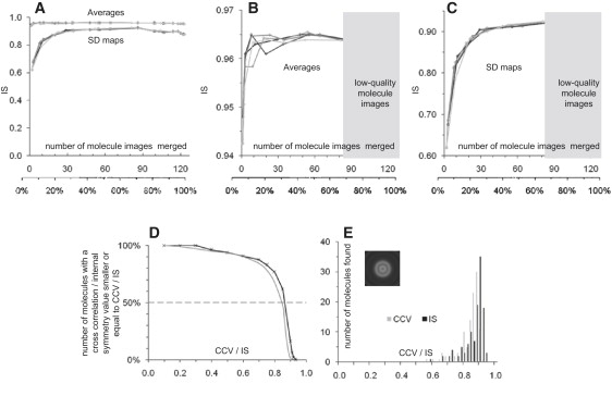
IS. (A) Averages have higher IS than SD maps (averages ∼0.96; SD maps ∼0.90). (B) Averages calculated from a few (2 or 3) molecule images are as symmetrical (0.965) as averages calculated from up to 65 molecule images. However inclusion of all molecules in an average drops the IS as the quality of merged images decreases. Best single-molecule images have an IS of ∼0.95. (C) For topographs acquired under similar conditions and displaying similar image quality as the topograph analyzed here, SD maps, emphasizing nonpreserved features in the molecule images, must contain at least ∼30 molecule images to reveal a highest IS of ∼0.90. Low-quality images contain object-unrelated distortions, and the integration of these drops the IS of the SD maps. (D) Graph displaying the number of molecules selected in the image shown in Fig. 1C as a function of IS used as criterion. The gray line documents the number of molecules found as a function of the CCV. (E) Histograms of all molecules found in the image versus the IS peaking at 0.90 ± 0.02 and the CCV peaking at 0.88 ± 0.02. (inset) 360-fold symmetrized particle used as reference for defining the molecules' oligomeric center.

After having found that only high-quality molecule images should be merged in averages and SD maps, we evaluated how IS can be used as selection criterion. For this, we analyzed the IS of all molecules in a raw data topograph (see Fig. 1 C) using the following approach: First, we used a 360-fold symmetrized molecule image as a reference (Fig. 2 E, inset) for peak search (any artificial object that defines the molecules' oligomeric centers is suitable). Second, the IS of all molecule images found was calculated. We plotted the number of molecules found versus the IS used as criterion (Fig. 2 D). The IS graph strongly resembles the CCV graph (see also Fig. 1 D). An IS histogram peaked at 0.90, showing that the best 50% of molecules are highly symmetrical (Fig. 2 E). The IS, as well as the CCV histograms, were well fitted by Gaussians, except for the shoulders toward low IS and CCV. These findings showed that the use of IS as a molecule image selection criterion led to similar results as the CCV approach. However, artifact-subjected molecules cannot necessarily be discriminated using a CCV approach, because the majority of molecules may be subject to the same irregularities, and a high similarity (CCV) between a reference and molecules may be found. Hence, the IS is a better particle selection criterion for AFM.

A novel feature-based lateral resolution analysis

To assess the imaging resolution in AFM, classical resolution determination methods developed for EM were used widely. However, as we show in this section, the results from these resolution assessments are problematic. Here, we propose a novel feature-based lateral resolution analysis method.

Classical single particle EM resolution determination methods are the DPR (17), the FRC (18), FSC for 3D data sets, and the SSNR (19,20). The DPR method divides the particles into two equal classes, averages each class, and compares the average phase in spatial frequency ranges—the resolution cutoff is defined as the spatial frequency where the phase discrepancy exceeds 45°. The FRC method also divides the particles into two equal classes, averages each class, and compares the cross-correlation of annular samplings of spatial frequency ranges of the two averages; the resolution cutoff is defined as the spatial frequency where the cross-correlation is negligible. The SSNR method is based on measuring the SNR as a function of the spatial frequency by comparing each particle with the ensemble average; the resolution cutoff is defined as the spatial frequency where the SNR is unacceptably low, for example, 4. AFM raw data images have a tremendous SNR, and therefore these criteria often provided doubtful results, indicating structural information to the Nyquist frequency (21). As shown above, many individual molecules have CCVs of ∼0.9 compared with averages, and two independently calculated averages, even if both comprise only a few molecules, are essentially the same (CCV ∼0.99). Therefore, EM single particle resolution determination methods find that high-quality AFM topographs are basically noise free and contain information to the Nyquist frequency. However, this does not necessarily mean high lateral resolution. In AFM imaging, the limiting factor is not noise but the effects of tip-contouring and tip-sample interaction.

Alternatively, often the observation of outermost diffraction spots in calculated power spectra was used to estimate the AFM imaging resolution of highly ordered 2D crystals (21). Unfortunately, phase reliability and completeness of high-frequency power spectra spots were never assessed thoroughly. A solitary visible reflection on the reciprocal lattice is likely to give an overly optimistic value of resolution (19). Additionally, this approach adapted from electron crystallography is limited in AFM because of the unknown CTF. Furthermore, tip contouring on a periodic sample may account for the appearance of high-frequency diffraction spots in calculated power spectra that do not correspond to structural details (Fig. 3); as an example, a tip of realistic diameter (Fig. 3 A) contours surface features separated by a distance slightly larger than the tip (Fig. 3 B, top). As the tip scans these features, a topography trace is recorded (Fig. 3 B, bottom). The interspace between the features may be small and may appear as high-frequency structure factors in calculated power spectra (Fig. 3 C). The illustration (Fig. 3) does not account for local effects (surface chemistry, charge, hydration); however, these effects do not change the described rationale: the schematic surface presentation can be understood as an iso-force surface structure.

Figure 3.

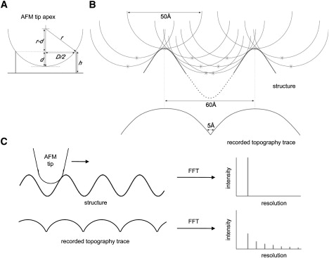
Tip size and tip contouring on periodic samples may account for high-frequency diffraction spots. (A) The tip radius r can be estimated through measuring the depth d inside barrel-shaped molecules (e.g., LH2 (34,41)) with diameter D. (B) Two surface features are separated by a distance slightly larger than the tip diameter. As the tip scans these features (consecutive tip positions are displayed by asterisks), a topography trace is recorded. The tip diameter of ∼50 Å and the distance between features of ∼60 Å are realistic values (note the unit cells of many 2D crystals are in this range; BR: 62.5 Å (42), AQP0: 65 Å (21)). (C) The interspace between features in the recorded topography may be small and appear as high-frequency structure factors in calculated power spectra even though the sample structure does not contain such small interspaces.

In light of the above outlined criticisms, we suggest a novel feature-based approach to assess the lateral resolution of AFM topographs, applicable to ensemble averages and to single-molecule images.

The rationale is the following: An average or single-molecule image is low-pass filtered Fourier ring by Fourier ring from the highest (Nyquist) frequency toward low frequency (Fig. 4, step 1). From each filtering round, a back-transformation is calculated and correlated with the original image (Fig. 4, step 2). The ACVs are plotted as a function of the low-pass cut-off. We hypothesized that the ACV drops significantly in resolution regimes when significant topographical features are cut off. This is observable by kinks in the ACV versus resolution graph (Fig. 4, inset). To highlight these kinks, we calculated the first derivative of the graph.

Figure 4.

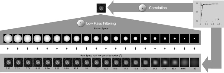
Feature-based lateral resolution analysis. Workflow of resolution analysis: (1) Low-pass filtering of input image corresponding to the maximal resolution pass shown underneath the back-transformed images. (2) Calculation of ACVs of each low-pass filtered image with the input image allows plotting an ACV versus resolution graph.

Here, we performed the above-described procedure (Fig. 4) using the 10 best single-molecule images of AqpZ (selected in Fig. 1 C following the IS criteria described in Fig. 2 D) and the average of these 10 molecule images (Fig. 5 A). The ACVs between the image and its low-pass filtered counterparts decreased rather slowly until ∼10 Å (0.10 Å^-1), when its slope got steeper and finally peaked in a maximum of the first derivative of the ACV plot at 11 Å (0.09 Å^-1). In other words, the cross correlation between the image and its low-pass filtered counterpart does not change significantly until a minimal feature size of ∼10 Å is reached. Therefore, we conclude that AqpZ images studied here do not contain significant structural information smaller than 10 Å. We define the resolution cut-off to the highest frequency where the ACV drops significantly. The frequency ranges where the ACV dropped contained structural information (Fig. 5 B, gray shaded). This information is repartitioned in resolution ranges: 50 Å–100 Å (approximately the size of AqpZ tetramer), 25 Å–38 Å (approximately the size of protein monomer), 16 Å–22 Å (approximately the size of surface loops), and 10–to 14 Å (approximately the size of fine details).

Figure 5.

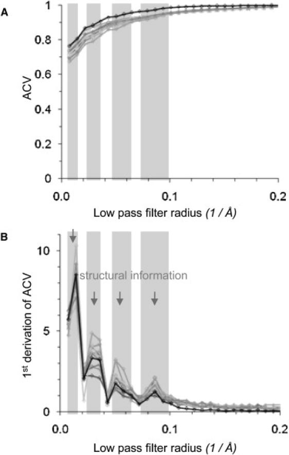
Resolution assessment for high-resolution AFM topographs of AqpZ. (A) Plot of ACV versus minimal feature size pass filtering (black: average image of the 10 best single molecules; gray: single molecules). At ∼0.1 Å^-1 (10 Å) the slope increases (gray shade). (B) Plot of first derivative of ACV versus minimal feature size. Structural information is contained in the gray-shaded resolution regimes (between 0.100 Å^-1 (10 Å) and 0.072 Å^-1 (14 Å), between 0.064 Å^-1 (16 Å) and 0.046 Å^-1 (22 Å), between 0.040 Å^-1 (25 Å) and 0.026 Å^-1 (38 Å), and between 0.020 Å^-1 (50 Å) and 0.010 Å^-1 (100 Å)).

Single-molecule versus average images

To assess the structural information in AFM topographs as a function of the number of molecule images averaged, we first analyzed the total height range of single-molecule and average images. Second, we compared the structural information revealed by single-molecule and average images with the atomic structure of AqpZ derived from x-ray diffraction of 3D crystals (29).

We examined the height ranges of averages calculated through merging different numbers of single-molecule images. We found that the gray-scale range, i.e., height scale, increased significantly when less molecule images were merged (Fig. 6 A). The height range resulted in 8.5 Å for the ensemble average of all 127 molecules, 9 Å when 64 (∼50%) molecules were averaged, 11 Å when only 3 molecule images were merged, and 12 ± 1 Å on the best single molecules (Fig. 6 C). The gray-scale range of the SD maps (Fig. 6 B), i.e., SD value range, is 2 Å when between ∼30 and all molecules were merged (Fig. 6 C). If <30 molecules were merged, the SD range increases up to 4 Å; however, the SD-map of only a few images has low IS (see Fig. 2) and no significance.

Figure 6.

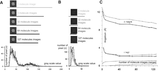
Height range of averages and SD value range of SD maps. (A) Gray value histograms of 8-bit gray-scale tiff averages (calculated from an image with 15 Å full gray scale, see Fig. 1C) of all molecules images (black) to one single-molecule image (light gray). The more molecule images are merged, the narrower the gray value range of the average image (bars underneath the images). (B) Gray value histograms of 8-bit gray-scale tiff SD maps (calculated from the same image as the averages in A of all molecule images (black) to three molecule images (light gray). The more molecule images are merged, the narrower the gray value range of the SD image (bars underneath the images). (C) Graph displaying base and top (average images: light gray diamonds; SD images: light gray circles), and the full height/value range (average images: dark gray diamonds; SD images: dark gray circles) as a function of the number of molecule images merged.

Why is the full height range of the ensemble average compressed by ∼30% compared with the average of the full height ranges of individual molecules? A protein surface that is not exposed to a loading force has a full height range h_(real) between the top protruding domains and the limiting bilayer surface (see Fig. S1 in the Supporting Material). Because of the tip geometry that often prohibits the penetration of the tip between densely located protrusions, a theoretical reduced height range h_(theo) is measured. When loading forces are applied, protruding domains are squeezed (34), and again, reduced height range h_(mes) is measured. In some rare cases, molecules are contoured at minimal loading forces, or at least some of their protrusions, and the tip penetrates to the bilayer. However, averaging of aligned molecules will merge full protrusions with squeezed protrusions and lipid bilayer depth with prohibited penetration and result in a reduced nonrealistic height range.

To evaluate the result of the height analysis, we compared the AFM measure of the surface hydrophilicity/hydrophobicity profile normal with the membrane plane of the AqpZ atomic structure (PDB 1RC2 (29)). For this, we colored the hydrophobic amino acids in red and hydrophilic amino acids in blue on the AqpZ surface (Fig. 7 A) and plotted their normalized surface coverage as a function of distance from the extracellular surface (Fig. 7 B). We found that the predominance of hydrophilic and hydrophobic surface properties changes at a height of ∼12 Å, the supposed level of the lipid bilayer surface. This is in agreement with the protrusion measurements on single molecules, represented on the AqpZ structure (Fig. 7 C). We conclude that the precise AFM height measure of a biomolecule is the average of the height ranges of the best molecules and not the height range of the average of the molecules.

Figure 7.

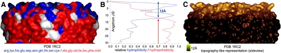
Membrane protruding domains in the AqpZ atomic structure (PDB 1RC2 (29)). (A) Surface representation of the atomic structure with hydrophilic and hydrophobic surface exposed amino acids colored in blue and red, respectively. (B) Plot of the relative surface coverage of hydrophilic and hydrophobic amino acids, indicating 12 Å hydrophilic membrane protruding protein structure on the extracellular surface. (C) Surface representation of the atomic structure with AFM color code covering the imaged area protruding 12 Å from black to gold.

After having seen that averaging downsizes the z-dimension of AFM topographs, we analyzed whether averaging has an impact on the resolution of structural details visible in x- and y-dimensions. We compared single-molecule and average images. The more images were merged, the more the structural details were blurred (Fig. 8 A). This was probably because structurally flexible protein details were not at the same position in all single-molecule images. A simple method to assess the variability of the images is to calculate the CCV between single molecules or independent averages merged from different numbers of molecules. The more molecules were merged, the higher the similarity (CCV) of the independent averages (1 molecule: 0.86; 3 molecules: 0.94; 5 molecules: 0.96; 10 molecules: 0.97; 50 molecules: 0.99).

Figure 8.

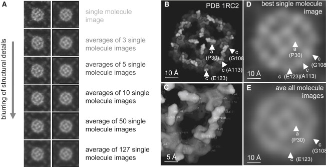
Structural features of single-molecule and average images of AqpZ. (A) Averaging of images may result in blurring of structural details (from top to bottom: single molecule to ensemble average images (left), fourfold symmetrized images (right)). (B) Surface representation of the atomic structure (PDB 1RC2 (29)). The top 12 Å of the model surface on the extracellular surface are colored from white to black following the z-coordinates. (C) Close view of one monomer in B, with the amino acids labeled. (D) The best single molecule. (E) Ensemble average. The protrusion around Ala113 in the middle of the c-loop is not detectable.

To evaluate what structural details are visible in AFM topographs, we compared the high-resolution AFM surface of AqpZ (25) with the atomic structure from x-ray diffraction of 3D crystals (29) (Fig. 8 B). The AqpZ structure, colored from bright to dark as a function of the z-axis position of the atoms similar to AFM topographs, reveals three major features per monomer on the extracellular surface (Fig. 8 C): the a-loop peaking at Pro30 and the c-loop that is strongly protruding at the beginning Gly108 and at the end Glu123. Close inspection of the x-ray structure showed that the elongated c-loop protrudes also in its middle at Ala113. Comparison of the best single-molecule topograph (Fig. 8 D) and the ensemble average (Fig. 8 E) showed once more that averaging blurs out structural features. Indeed, probably because of the flexibility of the proteins imaged at room temperature and in buffer solution, merging of no more than three molecules rendered the detection of the central c-loop protrusion at Ala113 difficult, whereas this protrusion is visible in best single molecules.

Conclusions

The detailed analyses of noise and distortions, IS, resolution, and averaging have been applied to high-resolution AFM topographs of different proteins, AqpZ (Figs. 1,2,5,6), AQP0 (6,35,36), AQP2 (37), and LH2 (7,38) (Figs. S2–S4), thereby showing the general applicability of the methods introduced here.

AFM is, to date, the only technique that is able to visualize the supramolecular assemblies of proteins directly in native membranes (6,7,40). However, often, AFM data is criticized because of its invasive tip-scanning mechanism. Skeptical researchers may think that the tip-sample interaction disturbs the molecular structure. Here, we showed this is not the case: best images from single n-oligomeric molecules have n-fold IS of up to 0.95. We also found that good single-molecule images are only minimally overlaid by noise. This makes AFM a unique tool for visualizing individual molecules.

High CCV with the ensemble reference is a useful molecule-selection criterion, but we present high IS to be the preferable approach to select best molecules in high-resolution topographs, because this approach allows distinguishing imaging artifacts like scan lines or directional deformation.

Because the use of resolution determination methods taken over from EM is problematic for AFM, in this work we suggest a novel feature-based analysis that can be used on single-molecule images with high signal. The lateral resolution values found range from 10 Å to 20 Å, depending on the proteins. The structural information-based resolution assessment is in agreement with data from other techniques.

Studying the effects of averaging on AFM topographs, we found that averaging compresses the protrusion dimension. Additionally, averaging blurs structural details. We conclude that best single-molecule images contain more structural information and reflect the protrusion height better than averages. This makes the AFM once more a key technique for single-molecule analysis.

References

- 1.Binnig G., Quate C.F., Gerber C. Atomic force microscope. Phys. Rev. Lett. 1986;56:930–933. doi: 10.1103/PhysRevLett.56.930. [DOI] [PubMed] [Google Scholar]
- 2.Engel A. Robert Feulgen lecture. Microscopic assessment of membrane protein structure and function. Histochem. Cell Biol. 2003;120:93–102. doi: 10.1007/s00418-003-0560-1. [DOI] [PubMed] [Google Scholar]
- 3.Schabert F.A., Henn C., Engel A. Native Escherichia coli OmpF porin surfaces probed by atomic force microscopy. Science. 1995;268:92–94. doi: 10.1126/science.7701347. [DOI] [PubMed] [Google Scholar]
- 4.Seelert H., Poetsch A., Dencher N.A., Engel A., Stahlberg H. Proton powered turbine of a plant motor. Nature. 2000;405:418–419. doi: 10.1038/35013148. [DOI] [PubMed] [Google Scholar]
- 5.Fotiadis D., Liang Y., Filipek S., Saperstein D.A., Engel A. Atomic-force microscopy: Rhodopsin dimers in native disc membranes. Nature. 2003;421:127–128. doi: 10.1038/421127a. [DOI] [PubMed] [Google Scholar]
- 6.Buzhynskyy N., Hite R.K., Walz T., Scheuring S. The supramolecular architecture of junctional microdomains in native lens membranes. EMBO Rep. 2007;8:51–55. doi: 10.1038/sj.embor.7400858. [DOI] [PMC free article] [PubMed] [Google Scholar]
- 7.Scheuring S., Sturgis J.N. Chromatic adaptation of photosynthetic membranes. Science. 2005;309:484–487. doi: 10.1126/science.1110879. [DOI] [PubMed] [Google Scholar]
- 8.Scheuring S., Boudier T., Sturgis J.N. From high-resolution AFM topographs to atomic models of supramolecular assemblies. J. Struct. Biol. 2007;159:268–276. doi: 10.1016/j.jsb.2007.01.021. [DOI] [PubMed] [Google Scholar]
- 9.Scheuring S., Buzhynskyy N., Jaroslawski S., Gonçalves R.P., Hite R.K. Structural models of the supramolecular organization of AQP0 and connexons in junctional microdomains. J. Struct. Biol. 2007;160:385–394. doi: 10.1016/j.jsb.2007.07.009. [DOI] [PubMed] [Google Scholar]
- 10.Cordier F., Barfield M., Grzesiek S. Direct observation of Calpha-Halpha...O=C hydrogen bonds in proteins by interresidue h3JCalphaC' scalar couplings. J. Am. Chem. Soc. 2003;125:15750–15751. doi: 10.1021/ja038616m. [DOI] [PubMed] [Google Scholar]
- 11.Lee J., Kozono D., Remis J., Kitagawa Y., Agre P. Structural basis for conductance by the archaeal aquaporin AqpM at 1.68 Å. Proc. Natl. Acad. Sci. USA. 2005;102:18932–18937. doi: 10.1073/pnas.0509469102. [DOI] [PMC free article] [PubMed] [Google Scholar]
- 12.Kimura K., Vassylev D.G., Miyazawa A., Kidera A., Matsushima M. Surface of bacteriorhodopsin revealed by high-resolution electron microscopy. Nature. 1997;389:206–211. doi: 10.1038/38323. [DOI] [PubMed] [Google Scholar]
- 13.Frank J. Electron microscopy of functional ribosome complexes. Biopolymers. 2003;68:223–233. doi: 10.1002/bip.10210. [DOI] [PubMed] [Google Scholar]
- 14.Simpson A., Chipman P., Baker T., Tijssen P., Rossmann M. The structure of an insect parvovirus (Galleria mellonella densovirus) at 3.7 A resolution. Structure. 1998;6:1355–1367. doi: 10.1016/s0969-2126(98)00136-1. [DOI] [PMC free article] [PubMed] [Google Scholar]
- 15.Standfuss J., Terwisscha van Scheltinga A.C., Lamborghini M., Kühlbrandt W. Mechanisms of photoprotection and nonphotochemical quenching in pea light harvesting complex at 2.5 A resolution. EMBO J. 2005;24:919–928. doi: 10.1038/sj.emboj.7600585. [DOI] [PMC free article] [PubMed] [Google Scholar]
- 16.Fotiadis D., Engel A. High-resolution imaging of bacteriorhodopsin by atomic force microscopy. Methods Mol. Biol. 2004;242:291–303. doi: 10.1385/1-59259-647-9:291. [DOI] [PubMed] [Google Scholar]
- 17.Frank J., Verschoor A., Boublik M. Computer averaging of electron micropgraphs of 40S ribosomal subunits. Science. 1981;214:1353–1355. doi: 10.1126/science.7313694. [DOI] [PubMed] [Google Scholar]
- 18.Saxton W.O., Baumeister W. The correlation averaging of a regularly arranged bacterial cell envelope protein. J. Microsc. 1982;127:127–138. doi: 10.1111/j.1365-2818.1982.tb00405.x. [DOI] [PubMed] [Google Scholar]
- 19.Unser M., Trus B.L., Steven A.C. A new resolution criterion based on spectral signal-to-noise ratios. Ultramicroscopy. 1987;23:39–52. doi: 10.1016/0304-3991(87)90225-7. [DOI] [PubMed] [Google Scholar]
- 20.Unser M., Trus B.L., Frank J., Steven A.L. The spectral signal-to-noise ration resolution criterion: Computational efficiency and statistical precision. Ultramicroscopy. 1989;30:429–434. doi: 10.1016/0304-3991(89)90074-0. [DOI] [PubMed] [Google Scholar]
- 21.Fotiadis D., Hasler L., Müller D.J., Stahlberg H., Kistler J. Surface tongue-and-groove contours on lens MIP facilitate cell-to-cell adherence. J. Mol. Biol. 2000;300:779–789. doi: 10.1006/jmbi.2000.3920. [DOI] [PubMed] [Google Scholar]
- 22.Stahlberg H., Fotiadis D., Scheuring S., Remigy H., Braun T. Two-dimensional crystals: a powerful approach to assess structure, function and dynamics of membrane proteins. FEBS Lett. 2001;504:166–172. doi: 10.1016/s0014-5793(01)02746-6. [DOI] [PubMed] [Google Scholar]
- 23.Unwin P.N.T., Henderson R. Molecular structure determination by electron microscopy of unstained crystalline specimens. J. Mol. Biol. 1975;94:425–440. doi: 10.1016/0022-2836(75)90212-0. [DOI] [PubMed] [Google Scholar]
- 24.Henderson R., Unwin P.N.T. Three-dimensional model of purple membrane obtained by electron microscopy. Nature. 1975;257:28–32. doi: 10.1038/257028a0. [DOI] [PubMed] [Google Scholar]
- 25.Scheuring S., Ringler P., Borgina M., Stahlberg H., Müller D.J. High resolution topographs of the Escherichia coli waterchannel aquaporin Z. EMBO J. 1999;18:4981–4987. doi: 10.1093/emboj/18.18.4981. [DOI] [PMC free article] [PubMed] [Google Scholar]
- 26.Ringler P., Borgnia M.J., Stahlberg H., Maloney P.C., Agre P. Structure of the water channel AqpZ from Escherichia coli revealed by electron crystallography. J. Mol. Biol. 1999;291:1181–1190. doi: 10.1006/jmbi.1999.3031. [DOI] [PubMed] [Google Scholar]
- 27.Henderson R., Baldwin J.M., Ceska T.A., Zemlin F., Beckman E. Model for the structure of bacteriorhodopsin based on high-resolution electron cryo-microscopy. J. Mol. Biol. 1990;213:899–929. doi: 10.1016/S0022-2836(05)80271-2. [DOI] [PubMed] [Google Scholar]
- 28.Luecke H., Schobert B., Richter H.T., Cartailler J.P., Lanyi J.K. Structure of bacteriorhodopsin at 1.55 A resolution. J. Mol. Biol. 1999;291:899–911. doi: 10.1006/jmbi.1999.3027. [DOI] [PubMed] [Google Scholar]
- 29.Savage D.F., Egea P.F., Robles-Colmenares Y., O'Connell J.D., Stroud R.M. Architecture and selectivity in aquaporins: 2.5 a x-ray structure of aquaporin Z. PLoS Biol. 2003;1:334–340. doi: 10.1371/journal.pbio.0000072. [DOI] [PMC free article] [PubMed] [Google Scholar]
- 30.Gonen T., Cheng Y., Sliz P., Hiroaki Y., Fujiyoshi Y. Lipid-protein interactions in double-layered two-dimensional AQP0 crystals. Nature. 2005;438:633–638. doi: 10.1038/nature04321. [DOI] [PMC free article] [PubMed] [Google Scholar]
- 31.Harries W.E., Akhavan D., Miercke L.J., Khademi S., Stroud R.M. The channel architecture of aquaporin 0 at a 2.2-A resolution. Proc. Natl. Acad. Sci. USA. 2004;101:14045–14050. doi: 10.1073/pnas.0405274101. [DOI] [PMC free article] [PubMed] [Google Scholar]
- 32.Rasband, W.S. 1997–2005. ImageJ.U.S. National Institutes of Health, Bethesda, Maryland, USA, http://rsb.info.nih.gov/ij/.
- 33.Müller D.J., Fotiadis D., Engel A. Mapping flexible protein domains at subnanometer resolution with the AFM. FEBS Lett. 1998;430:105–111. doi: 10.1016/s0014-5793(98)00623-1. [DOI] [PubMed] [Google Scholar]
- 34.Scheuring S., Seguin J., Marco S., Lévy D., Breyton C. AFM characterization of tilt and intrinsic flexibility of Rhodobacter sphaeroides light harvesting complex 2 (LH2) J. Mol. Biol. 2003;325:569–580. doi: 10.1016/s0022-2836(02)01241-x. [DOI] [PubMed] [Google Scholar]
- 35.Buzhynskyy N., Girmens J.-F., Faigle W., Scheuring S. Human cataract lens membrane at subnanometer resolution. J. Mol. Biol. 2007;374:162–169. doi: 10.1016/j.jmb.2007.09.022. [DOI] [PubMed] [Google Scholar]
- 36.Mangenot S., Buzhynskyy N., Girmens J.-F., Scheuring S. Malformation of junctional microdomains in type II diabetic cataract lens membranes. Submitted. 2008 doi: 10.1007/s00424-008-0604-4. [DOI] [PubMed] [Google Scholar]
- 37.Schenk A.D., Werten P.J.L., Scheuring S., de Groot B.L., Müller S.A. The 4.5 A structure of human AQP2. J. Mol. Biol. 2005;350:278–289. doi: 10.1016/j.jmb.2005.04.030. [DOI] [PubMed] [Google Scholar]
- 38.Scheuring S., Rigaud J.-L., Sturgis J.N. Variable LH2 stoichiometry and core clustering in native membranes of Rhodospirillum photometricum. EMBO J. 2004;23:4127–4133. doi: 10.1038/sj.emboj.7600429. [DOI] [PMC free article] [PubMed] [Google Scholar]
- 39.Reference deleted in proof.
- 40.Scheuring S., Seguin J., Marco S., Levy D., Robert B. Nanodissection and high-resolution imaging of the Rhodopseudomonas viridis photosynthetic core-complex in native membranes by AFM. Proc. Natl. Acad. Sci. USA. 2003;100:1690–1693. doi: 10.1073/pnas.0437992100. [DOI] [PMC free article] [PubMed] [Google Scholar]
- 41.Scheuring S., Reiss-Husson F., Engel A., Rigaud J.-L., Ranck J.-L. High resolution topographs of the Rubrivivax gelatinosus light-harvesting complex 2. EMBO J. 2001;20:3029–3035. doi: 10.1093/emboj/20.12.3029. [DOI] [PMC free article] [PubMed] [Google Scholar]
- 42.Müller D.J., Schabert F.A., Büldt G., Engel A. Imaging purple membranes in aqueous solutions at subnanometer resolution by atomic force microscopy. Biophys. J. 1995;68:1681–1686. doi: 10.1016/S0006-3495(95)80345-0. [DOI] [PMC free article] [PubMed] [Google Scholar]
Associated Data
This section collects any data citations, data availability statements, or supplementary materials included in this article.