Balance point characterization of interstitial fluid volume regulation

Abstract

The individual processes involved in interstitial fluid volume and protein regulation (microvascular filtration, lymphatic return, and interstitial storage) are relatively simple, yet their interaction is exceedingly complex. There is a notable lack of a first-order, algebraic formula that relates interstitial fluid pressure and protein to critical parameters commonly used to characterize the movement of interstitial fluid and protein. Therefore, the purpose of the present study is to develop a simple, transparent, and general algebraic approach that predicts interstitial fluid pressure (P_i) and protein concentrations (C_i) that takes into consideration all three processes. Eight standard equations characterizing fluid and protein flux were solved simultaneously to yield algebraic equations for P_i and C_i as functions of parameters characterizing microvascular, interstitial, and lymphatic function. Equilibrium values of P_i and C_i arise as balance points from the graphical intersection of transmicrovascular and lymph flows (analogous to Guyton's classical cardiac output-venous return curves). This approach goes beyond describing interstitial fluid balance in terms of conservation of mass by introducing the concept of inflow and outflow resistances. Algebraic solutions demonstrate that P_i and C_i result from a ratio of the microvascular filtration coefficient (1/inflow resistance) and effective lymphatic resistance (outflow resistance), and P_i is unaffected by interstitial compliance. These simple algebraic solutions predict P_i and C_i that are consistent with reported measurements. The present work therefore presents a simple, transparent, and general balance point characterization of interstitial fluid balance resulting from the interaction of microvascular, interstitial, and lymphatic function.

Interstitial inflow: interstitial fluid pressure and protein concentration determine flow of microvascular fluid and proteins into the interstitium.

The fluid filtration rate across a microvascular membrane, originally described by the Starling Hypothesis (53), is a result of an imbalance between two competing forces: hydrostatic and colloid osmotic pressures (41, 47). A decrease in interstitial fluid pressure increases the hydrostatic pressure gradient, driving fluid into the interstitium. A decrease in interstitial protein concentration, however, increases the colloid osmotic pressure gradient, maintaining fluid in the microvasculature. The two structural parameters that modulate the effects of these forces are the microvascular filtration coefficient (K_f), characterizing the permeability to water, and the reflection coefficient (σ), characterizing the relative permeability to proteins. The protein transfer rate across a microvascular membrane, on the other hand, is a result of convection driven by fluid filtration and diffusion driven by a protein concentration gradient. A decrease in interstitial fluid pressure increases the fluid filtration rate, driving proteins into the interstitium via convection. A decrease in interstitial protein concentration increases the protein concentration gradient, driving proteins into the interstitium via diffusion. The two structural parameters that modulate the effects of these processes are the reflection coefficient (σ) and the product of microvascular protein permeability and the surface area (PS) (56). Interstitial fluid pressure and protein concentration thus play significant roles in transfer of both fluid and proteins. Perhaps the complexity of interstitial fluid and protein dynamics has made it too difficult to identify the separate effects of interstitial inflow and outflow on interstitial fluid pressure (P_i) and protein concentration (C_i) (2, 31). Typically, the values of P_i and C_i are assumed constant, i.e., unaffected by changes in interstitial inflow (14).

Interstitial outflow: interstitial fluid pressure determines flow of fluid and proteins out of the interstitium.

The lymphatic system drains fluid and proteins from the interstitium. Characterizing the behavior of a single lymphatic vessel is complicated by the interplay of its axial pressure gradient, transmural pressure, and endothelial shear stress (3, 23, 24, 34, 45). Characterizing the function of an entire lymphatic system, however, is relatively simple, since the lymphatic system pressure-flow relationship can be linear over a large range of pressures (5, 22, 23). As interstitial fluid pressure increases, the resulting increase in axial pressure gradients and transmural pressures act in concert to increase lymph flow (34). In a series of articles, Drake and Laine (12, 13, 15, 17, 38, 39) successfully characterized the lymphatic pressure-flow relationship with two empirically derived parameters: the effective lymphatic resistance (R_L) and the lymphatic pump pressure (P_p). A recent study related the values of R_L and P_p to the mechanical properties of lymphatic vessels, including vessel contractility and contraction frequency (50). Although investigators have used Drake and Laine's formulation to predict the interaction of one part of a lymphatic system with another (55), this simple description has not yet been used to address lymphatic-microvascular interaction. In fact, a significant number of studies neglect the effect of lymphatic function on interstitial fluid balance (14).

Conservation of mass: edema is conventionally characterized as an imbalance of interstitial inflow and outflow.

The process of interstitial fluid volume regulation is typically characterized by invoking the principle of conservation of mass. The difference between interstitial inflow and outflow rates determines the rate of change in interstitial fluid volume. That is, when the inflow rate is greater than the outflow rate, the interstitial fluid volume increases. Conversely, when the outflow rate is greater than the inflow rate, the interstitial fluid volume decreases. The principle of conservation of mass, however, is limited. For instance, if only microvascular filtration is elevated experimentally, then gravimetric approaches can be used to ascribe changes in interstitial fluid volume to changes in microvascular permeability (14). However, measurement of interstitial fluid volume alone does not reveal whether microvascular filtration has increased or lymphatic function has decreased. In fact, once edema is established, inflow is equal to outflow, and no information is available to determine whether microvascular or lymphatic function has been compromised. Furthermore, the amount of microvascular filtration and lymph flow in the steady state is not directly related to interstitial fluid volume; edema can be associated with both high and low flows (10). Finally, because both conservation of mass and balance of forces are necessary to characterize mechanical systems from fundamental principles (21), characterization of edema as a mismatch of inflow and outflow is theoretically incomplete. Taken together, conservation of mass is necessary, but not sufficient, to characterize interstitial fluid balance.

Interstitial storage: interstitial compliance is conventionally believed to determine interstitial fluid pressure.

The capacity of the interstitium to store fluid is a fundamental mechanical property characterized by the “interstitial compliance,” the slope of the interstitial fluid volume-pressure relationship (28, 51). Interstitial compliance is believed to play a fundamental role in interstitial fluid balance: it determines how much interstitial fluid volume rises with an increase in interstitial fluid pressure. Three related concepts follow. First, the extraordinarily high interstitial compliance reported for the lung may prevent complications arising from edema (28, 54). In this case, interstitial fluid volume can significantly increase without a concomitant increase in interstitial fluid pressure, thus preventing alveolar flooding (28, 54). Second, decreasing the effective interstitial compliance with compressive sleeves may reduce peripheral edema by raising interstitial fluid pressure (6, 9). In this case, reduction of interstitial fluid volume follows from diminished microvascular filtration and enhanced lymphatic drainage. Finally, increasing interstitial compliance with pharmacological agents or focal injury may induce edema by decreasing interstitial fluid pressure (52). In this case, the lower interstitial fluid pressure draws fluid into the interstitium from the microvascular space. Inherent in all three concepts, a change in interstitial compliance is believed to alter the equilibrium interstitial fluid pressure.

Limitations of conventional mathematical models of fluid balance.

The individual processes involved in interstitial fluid volume regulation (inflow, outflow, and storage) are relatively simple and can be expressed in terms of general algebraic formulas. Integrating them to predict interstitial fluid pressure and volume, however, has been problematic. The interaction is complicated by the presence of negative feedback; an increase in interstitial fluid volume limits microvascular filtration and enhances lymphatic drainage. Furthermore, the effect of lymphatic function has not been explicitly introduced into fluid-balance models, limiting the generality of the results. Furthermore, the accumulation of interstitial fluid volume and proteins introduces integrals that have required numerical solution. Taken together, there is a notable lack of a first-order, algebraic formula that relates interstitial volume to critical parameters commonly used to characterize the movement of interstitial fluid. Therefore, the purpose of the present study is to develop a simple, general, algebraic approach that predicts interstitial fluid pressure, volume, and protein concentration resulting from the interaction of microvascular, interstitial, and lymphatic function.

THEORY

Interstitial inflow of fluid.

The Starling-Landis Equation (Eq. 1) characterizes the fluid filtration rate (J_V) across microvascular membrane into the interstitium (41, 47). The transmicrovascular fluid flow rate is determined by the microvascular filtration coefficient (K_f) in response to effective microvascular driving pressure resulting from hydrostatic and colloid osmotic pressure gradients. The difference between microvascular (P_c) and interstitial (P_i) hydrostatic pressures tends to force fluid into the interstitium. The value of K_f depends on microvascular surface area and permeability to water. The difference between microvascular (Π_c) and interstitial (Π_i) colloid osmotic pressures tends to draw fluid in the opposite direction, from the interstitium into the microvessels. The reflection coefficient (σ) characterizes the relative permeability of the microvasculature to plasma proteins (having a value between 0 and 1) and thus modulates the contribution of colloid osmotic pressure to effective microvascular driving pressure.

(1)

To be consistent with the rest of the analysis, the Starling-Landis Equation is formulated in terms of plasma (C_c) and interstitial protein (C_i) concentration given by Eq. 2, which will be used henceforth.

(2)

When concentration is expressed in moles per kilogram, α can be estimated by R·T, where R is the ideal gas constant and T is absolute temperature (57). When concentration is expressed in milligrams per milliliter, an experimentally derived value for α is used (31, 32). Consistent with previous work (10), P_c, P_i, C_c, and C_i are considered variables, and K_f and σ are considered structural parameters.

Interstitial inflow of proteins.

The microvascular protein extravasation rate (J_sV) (i.e., the interstitial inflow of proteins) is characterized by using the linear Taylor-Granger Equation (Eq. 3) (2, 56). In this formulation, protein flux across microvascular membrane is determined by convective as well as diffusive processes. The microvascular fluid filtration rate (J_V) drives the convective transfer of proteins and is modified by C_c and σ. The protein concentration gradient across microvascular membrane (C_c − C_i) drives protein diffusion and is modified by the microvascular protein permeability-surface area product (PS).

(3)

Although this formulation is based on an approximation proposed by Kedem and Katchalsky (37) that treats diffusion and convection as independent processes, comparison with other formulations suggested that the Taylor-Granger formulation better approximates the well-accepted nonlinear Patlak-Hoffman (49) formulation (Eq. A2) than other reported formulas (see Appendix).

Interstitial outflow of fluid.

The Drake-Laine Equation (Eq. 4) characterizes lymphatic function by relating lymph flow rate (J_L) to an effective lymphatic driving pressure (12). This equation is based on the common assumption that there is no protein concentration gradient across the terminal lymphatic membrane, and only the hydrostatic pressure gradient across lymphatic vessels drives the lymph flow (2). Since lymphatic outlet pressure (P_out) is typically greater than interstitial fluid pressure (P_i), the difference in P_i and P_out tends to retard lymph flow. The value of (P_i + P_p) represents the lymphatic driving pressure and is composed of interstitial hydrostatic pressure and lymphatic pumping pressure (P_p). The effective lymphatic resistance (R_L) is the slope of the relationship between effective lymphatic driving pressure (P_i + P_p − P_out) and the resulting lymph flow.

(4)

In this formulation P_p and R_L are empirically derived parameters used to describe the lymphatic pressure-flow relationship (12) and are not necessarily equivalent to pressure developed by lymphatic vessel contraction or resistance to lymph flow. Recently, P_p and R_L were related to lymphatic contractility and contraction frequency (50). Since transserosal flow is ultimately collected by lymphatics and returned to systemic circulation, transserosal flow is accommodated by the Drake-Laine model (Eq. 4).

Interstitial outflow of proteins.

Without a protein concentration gradient across the terminal lymphatic membrane, lymph protein concentration would be equal to interstitial protein concentration. Furthermore, the interstitial outflow rate of proteins is determined by a convective process only. Using the Drake-Laine Equation (Eq. 4) to characterize the lymphatic fluid drainage rate (J_L) driving convection, the rate of lymphatic drainage of interstitial proteins (J_sL) can be described.

(5)

Conservation of mass.

Based on the principle of conservation of mass, the rate of change in interstitial fluid volume (V) is determined by the difference between interstitial inflow (J_V) and outflow (J_L) rates of fluid. Similarly, the rate of change in interstitial protein content (Q) is determined by the difference between interstitial inflow (J_sV) and outflow (J_sL) rates of proteins (Eq. 6).

(6a)

(6b)

In steady state, interstitial fluid volume and protein concentration cease to change, and thus dV/dt and dQ/dt both equal zero. Therefore, inflow is balanced with outflow, and J_V = J_L and J_sV = J_sL.

Characterizing interstitial storage.

The capacity of the interstitium to store fluid volume (V) is a fundamental mechanical property characterized by the “interstitial compliance” (ΔV/ΔP_i), the slope of the interstitial fluid volume-pressure relationship (28, 51). The relationship between interstitial fluid pressure and volume depends on tissue hydration level and can be highly nonlinear (28, 51). However, the interstitial fluid volume-pressure relationship has been approximated to be “piecewise linear,” a commonly used technique to deal with the effect of hydration on interstitial compliance (5, 8, 31). Typically, under normal conditions in the negative (subatmospheric) interstitial pressure range, interstitial fluid pressure is sensitive to changes in interstitial fluid volume (i.e., interstitial compliance is small) and the interstitial fluid volume-pressure relationship is represented by a linear relationship. With overhydration, however, interstitial pressure can become positive, and the interstitial compliance can become much larger. Thus, with significant edema, the sensitivity of interstitial fluid volume to interstitial fluid pressure is lost (28). To capture this behavior, the interstitial fluid volume-pressure relationship in this range can be represented by another linear relationship, with a higher slope representing higher interstitial compliance. While within a particular linear range, the rate of interstitial fluid volume accumulation is related to interstitial compliance and the rate change in interstitial fluid pressure, dP_i/dt (Eq. 7a).

(7a)

(7b)

Interstitial storage of proteins is characterized by the ratio of total interstitial protein (Q) and interstitial fluid volume (Eq. 7b).

METHODS

Approaches to solving equations.

The individual subsystems that govern interstitial fluid volume and protein are relatively simple (Eqs. 2–7). However, their interaction can be complex, given that there is inherent feedback in the system. Equations 2–7 were nonetheless solved two ways. First, it was assumed that the system is in steady state (i.e., J_V = J_L and J_sV = J_sL), and P_i and C_i were found analytically by simultaneously solving Eqs. 2–7 in terms of the structural parameters (K_f, R_L, α, σ, P_p) using standard algebraic methods. Second, it was assumed that the system is not in steady state. In this case, the system of equations must be solved numerically, and all parameter values must be defined explicitly. Values of parameters (K_f, σ, R_L, P_p) were collected from various publications (dog lung, Table 1). To illustrate the role of interstitial compliance, the response to a change in capillary pressure (P_c) was simulated for low and high initial values of interstitial compliance. Equations 2–7 were solved simultaneously using a standard Runge-Kutta method implemented in MatLab R2007a (MathWorks, 2007), and the resulting transient changes in interstitial fluid pressure and volume were plotted as a function of time.

Table 1.

Comparison between the predicted values of interstitial fluid pressure (P_i) and interstitial protein concentration (C_i) calculated from Eq. 8 and previously reported values

Animal Model	Intervention	Values of Other Parameters	Estimated		Measured
			Pi	Ci	Pi	Ci
Dog lung	Control	RL = 76 mmHg·min/ml·100 g (11), Kf = 0.07 ml/min·mmHg·100 g (16,30), Pc = 7 mmHg (22), Cc = 58 mg/ml (33), σ = 0.62 (48), PS = 0.07 ml/min·100 g (48), Pp = 20 mmHg, Pout = 2 mmHg	−2.2	31	−2.7 (42)	35 (33)
Dog skeletal muscle	Baseline	RL = 200 mmHg·min/ml·100 g (38), Kf = 0.007 ml/min·mmHg·100 g (4), Pc = 24 (20), Cc = 54 mg/ml (58), σ = 0.72 (48), PS = 0.03 ml/min·100 g (48), Pp = 25 mmHg, Pout = 2 mmHg	−0.4	23.3	−0.1 (58)	22.4 (58)
Dog liver	Control	RL = 74 mmHg·min/ml·100 g (38), Kf = 0.3 ml/min·mmHg·100 g (26), Pc = 7 mmHg (40), Cc = 60 mg/ml (40), σ = 0.02 (48), PS =1.6 ml/min·100 g (48), Pp = 20 mmHg, Pout = 2 mmHg	5.9	59.8	6 (40)	56.7 (40)
Dog small intestine	Control	RL = 34 mmHg·min/ml·100 g (38), Kf = 0.37 ml/min·mmHg·100 g (35), Pc = 10 (35), Cc = 60 mg/ml (40), σ = 0.7 (48), PS = 0.09 ml/min·100 g (25), Pp = 20 mmHg, Pout = 2 mmHg	−0.6	24.4	0 (36)
Sheep lung	Baseline	RL = 100 mmHg·min/ml·100 g (39), Kf = 0.014 ml/min·mmHg·100 g (18), Pc = 14.34 mmHg (18), Cc = 74 mg/ml (18), σ = 0.48 (48), PS = 0.02 ml/min·100 g (48), Pp = 20 mmHg, Pout = 2 mmHg	−2.4	42.5		44.7 (18)

Average difference in predicted and measured values of P_i and C_i is 0.3 ± 0.3 mmHg and 2.0 ± 1.6 mg/ml (means ± SD), respectively. Numbers in the parentheses represent the reference from which the parameter value was collected. Parameters R_L, K_f, P_c, C_c, σ, PS, P_p, and P_out are defined in Table 2. Values for P_p were assumed; α = 0.37 (31, 32).

Validation of model at steady state.

The resulting algebraic formulas representing steady state were used to predict steady-state values of P_i and C_i in different organs. The resulting estimates of P_i and C_i were then compared with previously reported values of P_i and C_i derived experimentally (18, 33, 36, 40, 42, 58). Values of parameters (K_f, σ, R_L, P_p) were collected from various publications that used similar experimental models and conditions (Table 1).

Sensitivity analysis.

To determine the sensitivity of predicted values to parameters, the effect of 10% variation in each parameter was determined on the estimation of P_i and J_L for the illustrative case of the dog lung (Table 2). While one parameter was varied by 10%, the remaining parameters were assumed constant and equal to those listed in Table 1.

Table 2.

Effect of variation in parameters on estimated P_i and J_L in dog lung

Parameter	Units	Change in Pi mmHg	Change in JL ml/min·100 g
Microvascular pressure (Pc)	mmHg	0.55	0.0071
Plasma protein concentration (Cc)	mg/ml	−0.48	−0.0062
Microvascular filtration coefficient (Kf)	ml/min·mmHg·100 g	0.22	0.0028
Microvascular reflection coefficient (σ)		−0.99	−0.0130
Surface area-protein permeability product (PS)	ml/min·100 g	0.12	0.0015
Effective lymphatic resistance (RL)	mmHg·min/ml·100 g	0.33	−0.0150
Lymphatic pumping pressure (Pp)	mmHg	−0.44	0.0205
Lymphatic outlet pressure (Pout)	mmHg	0.04	−0.0021

Relative sensitivity of P_i and J_L to variation in structural, as well as inflow and outflow parameters, is evaluated in dog lung using parameter values listed in Table 1. While the parameter under consideration was increased by 10%, other parameters were held constant. Changes in P_i and J_L were estimated using Eqs. 8a and 9a.

Comparison of model predictions to reported changes in interstitial fluid pressure.

To illustrate the ability of the model equations to capture transient behavior reported in the literature, data were digitized from Lund et al. (43). Briefly, data were obtained from interstitial fluid pressure measurements in skin subjected to burn injuries. To simulate this experiment, Eqs. 2–7 were solved numerically, assuming that interstitial compliance increased linearly for 15 min to a plateau, using the same numerical methods described above for a stepwise increase in P_c. A set of parameters were chosen to reproduce the steady-state interstitial fluid pressure (before injury) and the peak negative interstitial fluid pressure (after injury). The resulting interstitial fluid pressure was plotted as a function of time.

RESULTS

Graphical representation of steady state.

The steady-state values of P_i and C_i can be represented graphically using a standard balance-point approach (27, 29). For illustration purposes, Fig. 1 represents the interstitial fluid flow balance point. To construct it, first the relationship of P_i and J_V (Eq. 2) is plotted. Assuming that interstitial protein concentration is in equilibrium, this relationship is linear, with a slope of −K_f. The x-intercept represents the total effective microvascular driving pressure forcing fluid into the interstitium, P_c − σσ(C_c − C_i), and is equal to the value of P_i at which J_v = 0. Then the relationship of P_i and J_L (Eq. 4) is plotted. This relationship is also linear, and has a slope of 1/R_L. The x-intercept represents the total effective pressure hindering flow from the interstitium, P_out − P_p, and is equal to the value of P_i at which J_L = 0. The intersection represents graphically the balance point where equilibrium interstitial inflow is equal to equilibrium interstitial outflow (i.e., J_V = J_L). The intersection is equivalent to setting J_V = J_L and solving Eqs. 2 and 4 simultaneously (resulting in Eq. 8a). A similar process can be used to construct a graph illustrating the interstitial protein flow balance point from Eqs. 3 and 5. The graphical representation of steady state provides a means to comprehend the individual contributions to interstitial fluid balance, where intercepts represent effective driving pressures and slopes represent effective resistances to flow.

Fig. 1.

Graphical representation of the balance point concept applied to interstitial fluid flow. Continuous line represents the Starling-Landis relationship (Eq. 2) (41, 47), which predicts that as interstitial pressure (P_i) increases, transmicrovascular flow into the interstitium (J_V) decreases. The dotted line represents the Drake-Laine relationship (Eq. 4) (12), which predicts that as P_i increases, lymph flow from the interstitium (J_L) increases. Their intercepts represent equilibrium, where flow into the interstitium is equal to flow out of the interstitium (i.e., J_v = J_L). Dashed lines represent the steady-state values of P_i, J_L, and J_V, explicitly expressed by Eq. 8a. Intercepts and slopes are related to effective fluid-driving pressures and resistances to fluid flow. 1/K_f is the effective resistance to flow into the interstitium and R_L is the effective lymphatic resistance. P_c − ασ(C_c − C_i) represents the total effective pressure forcing fluid into the interstitium, where P_c is the capillary hydrostatic pressure and C_c − C_i is the difference between capillary and interstitial protein concentrations. P_out − P_p represents the total effective pressure hindering flow from the interstitium, where P_out is the lymphatic system outlet pressure (presumably central venous pressure) and P_p is the effective lymphatic pumping pressure.

Algebraic solutions characterizing equilibriums.

As steady state is reached, interstitial inflow rates are balanced with outflow rates, leading to constant interstitial fluid volume and protein content. The solutions for P_i (Eq. 8a) and C_i (Eq. 8b) were obtained by solving the relationships, J_V = J_L and J_sV = J_sL, respectively. Equation 8 characterizes interstitial fluid pressure and protein concentration as a function of structural parameters (K_f, R_L, α, σ, P_p) and inlet and outlet variables (P_c, C_c, P_out). Equation 8a provides solutions corresponding to the intersections illustrated graphically in Fig. 1.

(8a)

(8b)

Notably, interstitial compliance, does not appear in Eq. 8a, indicating that interstitial compliance has no effect on interstitial fluid pressure. If C_i were to be measured, Eq. 8a immediately yields a value of P_i. Conversely, if P_i were to be measured, Eq. 8b immediately yields a value of C_i. However, numerical approaches can be used to solve Eq. 8a and 8b simultaneously to yield values of P_i and C_i without these measurements. Substituting Eqs. 8a and 8b into Eqs. 4 and 5 yield equilibrium lymphatic flows of fluid and protein.

(9a)

(9b)

Validation of model in steady state.

Table 1 illustrates the comparison between interstitial fluid pressure and protein concentration estimates with experimental measurements. The predicted steady-state values of interstitial fluid pressure and protein concentration compared favorably to measured values across all animal models. The average errors in predicted interstitial fluid pressure and protein concentration for all animal models in Table 1 were 0.3 ± 0.3 mmHg and 2.0 ± 1.6 mg/ml (means ± SD), respectively.

Sensitivity analysis.

As each parameter was varied by 10%, estimated P_i and J_L also varied considerably (Table 2). However, it is evident that 10% increase in σ produced the largest change in estimated P_i and J_L. Notably, changes in the microvascular filtration (K_f) and the surface area-protein permeability product (PS) had relatively small effects on P_i and J_L. Also notable is that changes in capillary pressure (P_c) had a much greater effect than changes in lymphatic outlet pressure (P_out).

Role of interstitial compliance in interstitial fluid pressure and fluid volume regulation.

Figure 2 illustrates changes in interstitial fluid pressure and fluid volume as a function of interstitial compliance resulting from a step change in capillary pressure. Figure 2 presents three critical aspects. First, interstitial compliance has a major effect on steady-state interstitial fluid volume. A 10-fold increase in interstitial compliance from 0.06 to 0.6 ml/100 g·mmHg increases interstitial fluid volume ∼1.5-fold. Second, the value of interstitial compliance will determine how quickly the system will return to steady state after a perturbation. A 10-fold increase in interstitial compliance from 0.06 to 0.6 ml/100 g·mmHg prolongs the time required to reach the steady state from ∼50 to ∼300 min. Third, the steady-state pressure is unaffected by interstitial compliance. Figure 3 further illustrates the role of interstitial compliance on transient and steady-state interstitial fluid pressures. With an increase in interstitial compliance believed to occur with burn injuries (43), interstitial fluid pressure immediately falls and recovers exponentially. When only interstitial compliance changes, the steady-state interstitial fluid pressure returns to the initial value. Model results are qualitatively similar to the data derived experimentally from a 40% burn injury (Fig. 3), in which interstitial fluid pressure falls abruptly, recovers exponentially (time constant, ≈ 45 min), and returns to near initial values (43).

Fig. 2.

Changes in interstitial fluid volume and pressure in response to a step change in capillary pressure. Illustrated are the results of numerically solving Eqs. 2–7, assuming the parameter values in Table I. Values of interstitial compliance, ΔV/ΔP_i, affect the rate at which the system comes to steady state, as well as the steady-state interstitial fluid volume. A 10-fold increase in interstitial compliance results in ∼6-fold increase in time required to reach steady state and ∼1.5-fold increase in the steady-state volume. Interstitial compliance has no impact on steady-state interstitial fluid pressure.

Fig. 3.

Data originally reported in Lund et al. (43) was derived from a 40% burn injury in skin, which caused a rapid increase in interstitial compliance. The resulting interstitial fluid pressure (P_i) dropped rapidly, which is normalized here by the peak negative value (P_imin = −31 mmHg). The curve represents simulation of the effect of rapidly increasing interstitial compliance on interstitial fluid pressure found by numerically solving Eqs. 2–7. The set of model parameters was chosen such that Eq. 8 reproduced the reported steady-state interstitial fluid pressure before the burn injury (approximately −1.6 mmHg). The value of interstitial compliance was chosen to reproduce the reported value of P_imin. The resulting model parameters were P_c = 16 mmHg, C_c = 58 mg/ml, σ = 0.62, P_p = 20 mmHg, P_out = 2 mmHg, K_f = 0.02 ml/100g·mmHg·min, and R_L = 66 mmHg·min/ml·100 g. Increase in interstitial compliance causes interstitial fluid pressure to rapidly drop, and then recover to baseline values following an exponential time course (time constant, ≈45 min).

DISCUSSION

Reconceptualizing interstitial fluid balance with inflow and outflow resistances.

The present work derived a series of simple algebraic formulas characterizing interstitial fluid pressure and protein regulation by integrating simple equations (Eqs. 2–7) using the classical concepts of linearity and time invariance (10, 19). A singular benefit of expressing interstitial fluid pressure with an algebraic function is that it leads to a new framework to understand interstitial fluid balance. Figure 4 depicts interstitial fluid pressure (P_i) regulation in terms of fluid compartments under transient (Fig. 4A) and steady-state conditions (Fig. 4B). Under transient conditions, a greater interstitial inflow than outflow leads to an increase in interstitial fluid volume. In steady state, however, interstitial volume comes to a constant value, and inflow is equal to outflow. The present work reformulated the equations describing microvascular filtration as a ratio (10, 19) relating a microvascular driving pressure {[(P_c−P_i)−ασ (C_c−C_i)]} to an inlet flow (J_V). This ratio results in an effective resistance to microvascular filtration equal to 1/K_f. Similarly, Drake et al. (12) characterized lymphatic drainage as a ratio relating a lymphatic driving pressure (P_i + P_p − P_out) to an outlet flow (J_L), resulting in an effective lymphatic resistance (R_L) (Eq. 4). Interstitial compliance, relating interstitial fluid pressure to interstitial fluid volume, determines the interstitial capacitance (Eq. 7a). When combined, these three components suggest an electrical circuit analogy consisting of two resistances in series and a capacitor in parallel (Fig. 4A). The resulting R_L(ΔV/ΔP_i) time constant provides a cutoff frequency that is much lower (<<1 Hz) than either capillary or lymphatic pressure oscillations, explaining in part why interstitial pressures typically lack pulsations. Under steady-state conditions, the electrical circuit analogy degenerates into a circuit consisting only of two resistances in series (Fig. 4B). Based on this electrical analogy, three insights become evident. First, the ratio of R_L and 1/K_f determines interstitial fluid pressure (Fig. 4B). In fact, the relative values of R_L and 1/K_f determine whether P_i approaches the microvascular driving pressure (when R_L>1/K_f) or effective lymphatic pumping pressure (when R_L<1/K_f) under steady state. Second, the sum of R_L and 1/K_f determines the total resistance and thus lymph flow. It thus becomes clear that interstitial fluid pressure can be regulated independently from transmicrovascular and lymph flow. Finally, there is a natural analogy to the classical description of capillary pressure regulation. Notably, capillary pressure also results from the ratio of inflow (arteriolar, R_a) and outflow (venular, R_v) resistances and is unaffected by (capillary) compliance (47).

Fig. 4.

Representation of interstitial fluid pressure (P_i) regulation in terms of both fluid compartments and an electrical analogy under transient (A) and steady-state conditions (B). With the electrical analogy, inlet resistance is equivalent to the inverse of the microvascular filtration coefficient (1/K_f), outlet resistance is equivalent to the effective lymphatic resistance (R_L), and capacitance is equivalent to the interstitial compliance (ΔV/ΔP_i). The effective inlet voltage is equivalent to [P_c − ασ(C_c − C_i)], which depends on capillary pressure (P_c), the reflection coefficient (σ), and the difference in capillary and interstitial protein concentrations (C_c − C_i). The effective outlet voltage is equivalent to (P_out − P_p), which depends on the lymphatic outlet pressure (P_out) and the effective lymphatic pump pressure (P_p). Under transient conditions, when interstitial inflow is greater than outflow, interstitial fluid volume increases. In this case, interstitial compliance affects transient changes in P_i. At steady state, inflow equals outflow, and interstitial compliance ceases to affect P_i. In this case, the ratio of 1/K_f and R_L determines whether P_i approaches microvascular driving pressure [P_c − ασ(C_c − C_i)] or effective lymphatic pumping pressure (P_out − P_p).

Steady-state interstitial fluid pressure is not affected by interstitial compliance.

The belief that interstitial compliance affects interstitial fluid pressure can be traced to the original work of Guyton (28). Clearly, interstitial compliance by definition relates a change in interstitial fluid volume to a change in interstitial fluid pressure. Therefore, transient changes in interstitial fluid pressure and volume are sensitive to interstitial compliance (Fig. 2). However, the present work demonstrates that the absolute value of interstitial fluid pressure in steady state is not affected by interstitial compliance (Eq. 8a). Steady-state interstitial fluid pressure is only a function of the resistances to interstitial inflow and outflow of fluid (1/K_f and R_L) and driving pressures {[P_c−ασ (C_c−C_i)] and [P_out−P_p]} (Fig. 4B). Once interstitial fluid pressure is determined by the ratio of inflow and outflow resistances, interstitial storage capacity, characterized by the interstitial fluid volume-pressure relationship, determines the corresponding interstitial fluid volume. Although interstitial compliance does not affect steady-state interstitial fluid pressure, it nonetheless determines the time required to reach steady state and the ultimate interstitial volume (Fig. 2). In the case of pulmonary edema, for instance, a relatively high interstitial compliance can prolong the time before an edemagenic challenge increases interstitial pressure and causes alveolar flooding. Although higher interstitial compliance increases the lung's edemagenic gain (10), it may provide the system enough time to resolve the primary cause of increased microvascular flux.

Validity of assumptions.

To arrive at the simple algebraic solutions in the present work (Eq. 8), a number of assumptions were required. The first set included assumptions that are commonly made when modeling microvascular filtration. Focusing on whole organ fluid balance, the common assumption was made that the interstitial space within an organ behaves as a well-mixed compartment; there is no protein concentration gradient across the interstitial space (56). This assumption may result in an overestimation of the flow of fluid and proteins across microvascular membranes when microvascular filtration is low (56). Although several equations are reported that describe microvascular protein extravasation, the Taylor-Granger Equation (Eq. 3) (56) was selected, because it is relatively simple and has been experimentally validated. This equation tends to overestimate microvascular protein extravasation when microvascular filtration is low, but approaches the well-accepted nonlinear Patlak-Hoffman formulation (49) with increasing microvascular filtration (see appendix). A less common set of assumptions is required specifically for the present work. Although all variables characterizing microvascular, interstitial, and lymphatic function have nonlinear relationships, for conceptual clarity we elected to represent them with linear relationships (Eqs. 2–7). Linearization incurs minimal error if either of the variables vary within a small range or the relationships are treated as piecewise linear (5, 8, 31). The interstitial fluid volume-pressure relationship is particularly nonlinear, since the slope increases dramatically at higher hydration levels (28). This particular nonlinearity has minimal impact on Eq. 8, since interstitial compliance has no effect on steady-state interstitial fluid pressure. It may affect the predicted transient changes in interstitial fluid pressures illustrated in Fig. 3, however, since the range of interstitial fluid pressures is so large. Another critical assumption of linearity is embodied by the description of lymphatic function, appropriated from Drake et al. (12). Two critical parameters, R_L and P_p, were derived empirically, and represent the slope and intercept of the lymphatic outflow-pressure relationship. As has been argued previously (2), R_L and P_p do not represent the physical resistance to lymph flow or the pressure developed by lymphatic contractions. Recently, R_L and P_p have been revealed to be related to both lymphatic vessel contractility and contraction frequency (50). Furthermore, it is possible that the three parameters, the microvascular filtration coefficient, effective lymphatic resistance, and interstitial compliance, interact with each other, resulting in nonlinear behavior. For instance, changes in interstitial compliance may affect R_L by altering interstitial-lymphatic tethering. However, for the current linear analysis, these three parameters are assumed to be independent of each other. Also, parameters characterizing microvascular filtration are typically reported in units per weight. Because lymphatic parameters characterize whole-organ behavior, they must be normalized to make their units consistent. Perhaps the best indication that the assumptions made in the present work are reasonable is the comparison of model results with reported data.

Comparison of model results with reported data.

Both steady-state and transient model results were compared with reported data. To illustrate the ability of the resulting algebraic equations (Eq. 8) to predict interstitial fluid pressure and protein concentration, specific parameter values had to be assumed (Table 1). Because the parameter values reported from the literature resulted from different animal models, organ systems, and experimental interventions, their ranges were relatively large. The fact that predicted steady-state values of interstitial fluid pressure compared favorably to measured values (Table 1) provides the greatest argument for the validity of the assumptions used in the present work. Furthermore, the transient solution, solved for the case of change in interstitial compliance, mimics what has been reported for burn injuries (Fig. 3). In particular, the interstitial fluid pressures fell abruptly, rose exponentially (time constant, ≈ 45 min), and returned to baseline values. Small persistent deviations from baseline values may have been the result of confounding alterations in microvascular permeability (1, 46, 52). We can predict that as small as a 25% increase in the microvascular filtration coefficient or 50% increase in the effective lymphatic resistance after burn injury will result in this small deviation in steady-state interstitial fluid pressure.

Graphical balance point approach provides a tool to conceptualize complex problems.

The algebraic solutions developed in the present work (Eq. 8) are manifestations of a balance-point characterization of interstitial fluid volume and protein regulation. Like Guyton, who used a balance point approach to characterize venous return-cardiac output interaction (27, 29), we characterized microvascular-lymphatic interaction as equilibrium between the inflow and outflow of fluid and proteins (Figs. 1 and 5). Whereas numerical approaches to solve the interstitial fluid flow equations are powerful, the graphical balance point approach derived from Eqs. 2–4 is simple enough to reveal fundamental behaviors resulting from changes in slope or intercepts. Figure 5A illustrates that increasing K_f shifts the balance point (from A to B), yielding higher interstitial fluid pressure and lymph flow. Figure 5B illustrates that increasing R_L shifts the balance point, yielding higher interstitial fluid pressure and lower lymph flow. For instance, in the case of dog lung, a 10% increase in K_f increases P_i by 0.22 mmHg, whereas a 10% increase in R_L increases P_i by 0.33 mmHg (Table 2). Figure 5C illustrates that increasing capillary pressure (P_c) increases microvascular driving pressure that shifts the balance point, yielding higher interstitial fluid pressure and lymph flow. By increasing the microvascular driving pressure, a 10% increase in P_c increases P_i by 0.55 mmHg in dog lung. Figure 5D illustrates that increasing lymphatic outlet pressure (P_out) increases lymphatic effective pumping pressure that shifts the balance point, yielding higher interstitial fluid pressure and lower lymph flow. Perhaps more importantly, this graphical approach can reveal surprising behavior resulting from the interaction of parameters. For instance, although simultaneous increase in K_f and R_L (shifting the balance point from A to B in Fig. 5E) will yield higher interstitial fluid pressure, and thus volume, microvascular filtration and lymph flow can remain unchanged. In case of dog lung, 10% increase in K_f and 2% increase in R_L increases P_i by 0.28 mmHg, but leaves J_L unchanged. The common practice of using lymph flow to estimate K_f (14) may therefore fail, because the data simply does not contain enough information to make such a determination. Conversely, an increase in K_f, if accompanied by a decrease in R_L, (shifting the balance point from A to B in Fig. 5F) will yield increased microvascular and lymphatic flow without a corresponding change in interstitial fluid pressure. In fact, interstitial fluid volume would remain unchanged if interstitial compliance remained constant. In case of dog lung, 10% increase in K_f and 6% decrease in R_L increases J_L by 0.013 ml/min·100 g, but leaves P_i unchanged. Use of gravimetric approaches to infer changes in K_f (14) from steady-state interstitial fluid pressures and volumes would therefore fail, because the data does not contain enough information to make such a determination.

Fig. 5.

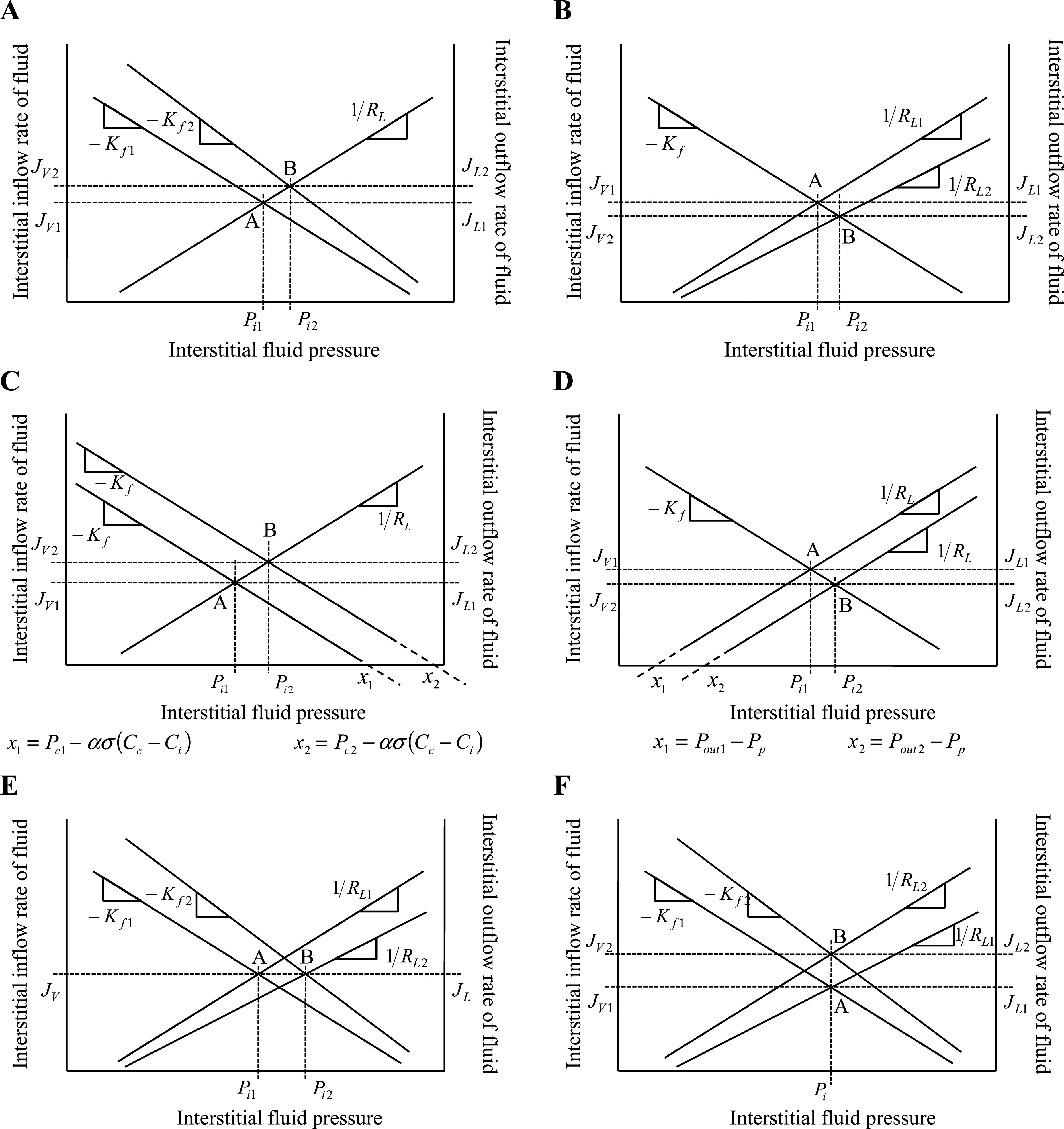
Illustration of the use of the graphical balance point analysis introduced in Fig. 1 to provide intuitive insight into interstitial fluid pressure regulation. Effect of changing various parameters and variables on interstitial fluid pressure (P_i), microvascular fluid filtration (J_V), and lymph outflow (J_L) is illustrated by a shift in the balance point from A to B. Subscripts indicate change from state 1 to state 2. A: increasing microvascular filtration coefficient (from K_f1 to K_f2) shifts the balance point from A to B and increases interstitial fluid pressure (from P_i1 to P_i2). B: increasing effective lymphatic resistance (from R_L1 to R_L2) shifts the balance point from A to B and increases interstitial fluid pressure (from P_i1 to P_i2). C: increasing capillary pressure (from P_c1 to P_c2) shifts the x-intercept from x₁ to x₂ and the balance point from A to B and results in higher interstitial fluid pressure (from P_i1 to P_i2). D: increasing lymphatic outlet pressure (from P_out1 to P_out2) shifts the x-intercept from x₁ to x₂ and the balance point from A to B and results in higher interstitial fluid pressure (from P_i1 to P_i2). E: concomitantly increasing K_f and R_L shifts the balance point from A to B and increases interstitial fluid pressure (from P_i1 to P_i2), but J_V and J_L are unaltered. F: simultaneously increasing K_f and decreasing R_L increases J_V and J_L, but maintains interstitial fluid pressure.

Perspectives and Significance

The present work provides a predictive characterization of interstitial fluid balance resulting from the interaction of microvascular, interstitial, and lymphatic function. This approach has made advances to conventional fluid balance models because it 1) does not neglect lymphatic function and its effect on interstitial fluid pressure, 2) does not assume that interstitial fluid pressure or protein concentration is constant, 3) characterizes fluid balance in terms of resistances to fluid transport, 4) provides a general algebraic solution in terms of microvascular and lymphatic parameters, and 5) provides a relatively simple analytical tool that may make the physics more accessible to physiologists and concepts of interstitial fluid balance accessible to students already familiar with the balance point concept. The resulting approach reveals that 1) steady-state interstitial fluid pressure depends on a simple multiplication of effective lymphatic resistance and the microvascular filtration coefficient, 2) interstitial compliance has no effect on steady-state interstitial fluid pressure, 3) interstitial pressure is more sensitive to changes in capillary pressure than lymphatic outlet pressure, 4) interstitial pressure is at least as sensitive (or possibly more sensitive) to changes in effective lymphatic resistance than the more commonly studied microvascular filtration coefficient, and 5) the practice of using lymph flow to estimate the microvascular filtration coefficient (14) may fail, because the data simply does not contain enough information to make such a determination. The present work, however, presents notable limitations that must be addressed in future work. First, all parameters used to validate the current model did not originate from the same study, which constrains the ability to identify model limitations. Second, the time course of edema formation is clinically relevant, and the balance point approach only characterizes the steady-state condition. Third, the common practice of using measured lymph protein concentration to estimate interstitial protein concentration can lead the model to overestimate the predicted value of interstitial fluid pressure. Fourth, the model has not yet been interrogated to explore how different species exhibit different adaptive strategies to achieve optimal fluid balance. Finally, the mathematical model of the present approach has not yet been applied to re-evaluate the conclusions drawn by numerous previous studies that use mathematical models of fluid balance to interpret their experimental results that are less comprehensive and make much more problematic assumptions.

GRANTS

Portions of this work were supported by National Heart, Lung, and Blood Institute Grants K25-HL-070608 (to C. M. Quick), American Heart Association Grants 0565116Y (to C. M. Quick), and 0365127Y (to R. H. Stewart), and Center for Disease Control Grant 623086 (to G. A. Laine).

APPENDIX

Nonlinear forms of the protein extravasation equation.

Based on the principles of irreversible thermodynamics, Kedem and Katchalsky (37) characterized solute transport across homoporous, sieving membranes (Eq. A1). In this formulation, the convective and diffusive processes responsible for protein extravasation are considered independent of each other. On the other hand, the Patlak-Hoffman formulation (Eq. A2) (49) considers simultaneous convection and diffusion of proteins through the same pathway. In fact, their formulation generalizes the Hertzian formulation for sieving membranes, recognized as the gold standard for nonsieving membranes (7). The Manning formulation (Eq. A3) (44) is a linear approximation of Patlak-Hoffman formulation, assuming small J_V. The Taylor-Granger formulation (Eq. 3) (56) is the linear empirical approximation of Kedem-Katchalsky formulation. Except for the Kedem-Katchalsky formulation, the two-well accepted formulations (Eqs. A2 and A3), along with Taylor-Granger formulation, suggest that C_L/C_c approaches (1−σ) with increasing J_V, i.e., lymph protein concentration (C_L), approaches a constant value at high J_V.

(A1)

(A2)

(A3)

Comparison of numerical solutions for protein extravasation.

Various comparative studies have reported the accuracy of different microvascular protein extravasation characterizations. One such study by Bresler and Groome (7) compared the Kedem-Katchlasky (37) and Manning (44) formulations to the Patlak-Hoffman formulation (49). The Taylor-Granger formulation (56) has not been included in such studies. In the present work, an approach similar to that of Bresler and Groome was used to compare the accuracy of the J_sV estimation by the Taylor-Granger formulation (Eq. 3) with those of Kedem-Katchlasky (Eq. A1), Patlak-Hoffman (Eq. A2), and Manning (Eq. A3). As reported by Bresler and Groome, the Patlak-Hoffman formulation is considered the gold standard for comparison purposes. The ratio of errors in J_sV estimation is determined with Eqs. A4a and A4b. Equation A4a compares the Taylor-Granger formulation with the Kedem-Katchlasky formulation, and Eq. A4b compares the Taylor-Granger formulation with the Manning formulation.

(A4a)

(A4b)

Figure 6 illustrates R1 (Fig. 6A) and R2 (Fig. 6B) as a function of J_V with C_i/C_c = 0.1, 0.5 and 0.9 (σ = 0.6, PS = 0.118). R1 is reduced as C_i approaches C_c. However, it can be shown by algebraically reducing Eq. A4b that R2 is independent of C_c or C_i and is therefore not affected by changes in C_i/C_c. The Taylor-Granger formulation (56) better approximates the Patlak-Hoffman formulation (49) with increasing J_V than the others.

Fig. 6.

Microvascular protein extravasation rate (J_sV) estimation using the Taylor-Granger formulation (J_sV^TG) (Eq. 3) (56) is compared with the Kedem-Katchalsky formulation (J_sV^KK) (Eq. A1) (37) and the Manning formulation (J_sV^M) (Eq. A3) (44) assuming the Patlak-Hoffman formulation (J_sV^PH) (Eq. A2) (49) is ideal (7). A: ratio of errors as a function of J_V compares the Taylor-Granger formulation with the Kedem-Katchalsky formulation assuming C_i/C_c = 0.1, 0.5 and 0.9 (σ = 0.6, PS = 0.118). B: ratio of errors as a function of J_V compares the Taylor-Granger formulation with the Manning formulation assuming C_i/C_c = 0.1, 0.5, and 0.9 (σ = 0.6, PS = 0.118). R1 is reduced as C_i approaches C_c. However, it can be shown by algebraically reducing Eq. A4b that R2 is independent of C_c or C_i and is therefore not affected by changes in C_i/C_c. The fact that R1 >1 and R2 >1 with increasing J_V suggests that the Taylor-Granger formulation is the best approximation of the Patlak-Hoffman formulation.

REFERENCES

- 1.Arturson G, Mellander S. Acute changes in capillary filtration and diffusion in experimental burn injury. Acta Physiol Scand 62: 457–463, 1964. [DOI] [PubMed] [Google Scholar]
- 2.Aukland K, Reed RK. Interstitial-lymphatic mechanisms in the control of extracellular fluid volume. Physiol Rev 73: 1–78, 1993. [DOI] [PubMed] [Google Scholar]
- 3.Benoit JN, Zawieja DC, Goodman AH, Granger HJ. Characterization of intact mesenteric lymphatic pump and its responsiveness to acute edemagenic stress. Am J Physiol Heart Circ Physiol 257: H2059–H2069, 1989. [DOI] [PubMed] [Google Scholar]
- 4.Bentzer P, Kongstad L, Grande PO. Capillary filtration coefficient is independent of number of perfused capillaries in cat skeletal muscle. Am J Physiol Heart Circ Physiol 280: H2697–H2706, 2001. [DOI] [PubMed] [Google Scholar]
- 5.Bert JL, Gyenge CC, Bowen BD, Reed RK, Lund T. A model of fluid and solute exchange in the human: validation and implications. Acta Physiol Scand 170: 201–209, 2000. [DOI] [PubMed] [Google Scholar]
- 6.Brennan MJ, Miller LT. Overview of treatment options and review of the current role and use of compression garments, intermittent pumps, and exercise in the management of lymphedema. Cancer 83: 2821–2827, 1998. [DOI] [PubMed] [Google Scholar]
- 7.Bresler EH, Groome LJ. On equations for combined convective and diffusive transport of neutral solute across porous membranes. Am J Physiol Renal Fluid Electrolyte Physiol 241: F469–F476, 1981. [DOI] [PubMed] [Google Scholar]
- 8.Chapple C, Bowen BD, Reed RK, Xie SL, Bert JL. A model of human microvascular exchange: parameter estimation based on normals and nephrotics. Comput Methods Programs Biomed 41: 33–54, 1993. [DOI] [PubMed] [Google Scholar]
- 9.Cheville AL, McGarvey CL, Petrek JA, Russo SA, Taylor ME, Thiadens SR. Lymphedema management. Semin Radiat Oncol 13: 290–301, 2003. [DOI] [PubMed] [Google Scholar]
- 10.Dongaonkar RM, Quick CM, Stewart RH, Drake RE, Cox CS Jr, Laine GA. Edemagenic gain and interstitial fluid volume regulation. Am J Physiol Regul Integr Comp Physiol 294: R651–R659, 2008. [DOI] [PubMed] [Google Scholar]
- 11.Drake RE, Adcock DK, Scott RL, Gabel JC. Effect of outflow pressure upon lymph flow from dog lungs. Circ Res 50: 865–869, 1982. [DOI] [PubMed] [Google Scholar]
- 12.Drake RE, Allen SJ, Katz J, Gabel JC, Laine GA. Equivalent circuit technique for lymph flow studies. Am J Physiol Heart Circ Physiol 251: H1090–H1094, 1986. [DOI] [PubMed] [Google Scholar]
- 13.Drake RE, Allen SJ, Williams JP, Laine GA, Gabel JC. Lymph flow from edematous dog lungs. J Appl Physiol 62: 2416–2420, 1987. [DOI] [PubMed] [Google Scholar]
- 14.Drake RE, Laine GA. Pulmonary microvascular permeability to fluid and macromolecules. J Appl Physiol 64: 487–501, 1988. [DOI] [PubMed] [Google Scholar]
- 15.Dunbar BS, Elk JR, Drake RE, Laine GA. Intestinal lymphatic flow during portal venous hypertension. Am J Physiol Gastrointest Liver Physiol 257: G94–G98, 1989. [DOI] [PubMed] [Google Scholar]
- 16.Ehrhart IC, Granger WM, Hofman WF. Filtration coefficient obtained by stepwise pressure elevation in isolated dog lung. J Appl Physiol 56: 862–867, 1984. [DOI] [PubMed] [Google Scholar]
- 17.Elk JR, Drake RE, Williams JP, Gabel JC, Laine GA. Lymphatic function in the liver after hepatic venous pressure elevation. Am J Physiol Gastrointest Liver Physiol 254: G748–G752, 1988. [DOI] [PubMed] [Google Scholar]
- 18.Erdmann AJ, Vaughan TR Jr, Brigham KL, Woolverton WC, Staub NC. Effect of increased vascular pressure on lung fluid balance in unanesthetized sheep. Circ Res 37: 271–284, 1975. [DOI] [PubMed] [Google Scholar]
- 19.Franklin GF, Powell JD, Abbas EN. Feedback Control of Dynamic Systems. Upper Saddle River, NJ: Prentice Hall, 2005.
- 20.Fronek K, Zweifach BW. Microvascular pressure distribution in skeletal muscle and the effect of vasodilation. Am J Physiol 228: 791–796, 1975. [DOI] [PubMed] [Google Scholar]
- 21.Fung YC Biomechanics: Mechanical Properties of Living Tissues. New York: Springer-Verlag, 1993.
- 22.Gaar KA, Taylor AE, Owens LJ, Guyton AC. Pulmonary capillary pressure and filtration coefficient in the isolated perfused lung. Am J Physiol 213: 910–914, 1967. [DOI] [PubMed] [Google Scholar]
- 23.Gashev AA, Davis MJ, Zawieja DC. Inhibition of the active lymph pump by flow in rat mesenteric lymphatics and thoracic duct. J Physiol 540: 1023–1037, 2002. [DOI] [PMC free article] [PubMed] [Google Scholar]
- 24.Gashev AA, Zawieja DC. Physiology of human lymphatic contractility: a historical perspective. Lymphology 34: 124–134, 2001. [PubMed] [Google Scholar]
- 25.Granger DN, Taylor AE. Permeability of intestinal capillaries to endogenous macromolecules. Am J Physiol Heart Circ Physiol 238: H457–H464, 1980. [DOI] [PubMed] [Google Scholar]
- 26.Greenway CV, Lautt WW. Effects of hepatic venous pressure on transsinusoidal fluid transfer in the liver of the anesthetized cat. Circ Res 26: 697–703, 1970. [DOI] [PubMed] [Google Scholar]
- 27.Guyton AC Determination of cardiac output by equating venous return curves with cardiac response curves. Physiol Rev 35: 123–129, 1955. [DOI] [PubMed] [Google Scholar]
- 28.Guyton AC Interstitial fluid pressure. II. Pressure-volume curves of interstitial space. Circ Res 16: 452–460, 1965. [DOI] [PubMed] [Google Scholar]
- 29.Guyton AC, Hall JE. Textbook of Medical Physiology. Philadelphia, PA: Saunders, 2000.
- 30.Guyton AC, Lindsey AW. Effect of elevated left atrial pressure and decreased plasma protein concentration on the development of pulmonary edema. Circ Res 7: 649–657, 1959. [DOI] [PubMed] [Google Scholar]
- 31.Gyenge CC, Bowen BD, Reed RK, Bert JL. Transport of fluid and solutes in the body. I. Formulation of a mathematical model. Am J Physiol Heart Circ Physiol 277: H1215–H1227, 1999. [DOI] [PubMed] [Google Scholar]
- 32.Gyenge CC, Bowen BD, Reed RK, Bert JL. Transport of fluid and solutes in the body. II. Model validation and implications. Am J Physiol Heart Circ Physiol 277: H1228–H1240, 1999. [DOI] [PubMed] [Google Scholar]
- 33.Hara N, Nagashima A, Yoshida T, Furukawa T, Inokuchi K. Effect of decreased plasma colloid osmotic pressure on development of pulmonary edema in dogs. Jpn J Surg 11: 203–208, 1981. [DOI] [PubMed] [Google Scholar]
- 34.Hargens AR, Zweifach BW. Contractile stimuli in collecting lymph vessels. Am J Physiol Heart Circ Physiol 233: H57–H65, 1977. [DOI] [PubMed] [Google Scholar]
- 35.Johnson PC, Hanson KM. Capillary filtration in the small intestine of the dog. Circ Res 19: 766–773, 1966. [DOI] [PubMed] [Google Scholar]
- 36.Johnson PC, Richardson DR. The influence of venous pressure on filtration forces in the intestine. Microvasc Res 7: 296–306, 1974. [DOI] [PubMed] [Google Scholar]
- 37.Kedem O, Katchalsky A. Thermodynamic analysis of the permeability of biological membranes to non-electrolytes. Biochim Biophys Acta 27: 229–246, 1958. [DOI] [PubMed] [Google Scholar]
- 38.Laine GA, Allen SJ, Katz J, Gabel JC, Drake RE. Outflow pressure reduces lymph flow rate from various tissues. Microvasc Res 33: 135–142, 1987. [DOI] [PubMed] [Google Scholar]
- 39.Laine GA, Drake RE, Zavisca FG, Gabel JC. Effect of lymphatic cannula outflow height on lung microvascular permeability estimations. J Appl Physiol 57: 1412–1416, 1984. [DOI] [PubMed] [Google Scholar]
- 40.Laine GA, Hall JT, Laine SH, Granger J. Transsinusoidal fluid dynamics in canine liver during venous hypertension. Circ Res 45: 317–323, 1979. [DOI] [PubMed] [Google Scholar]
- 41.Landis EM Micro-injection studies of capillary permeability: II. The relation between capillary pressure and the rate at which fluid passes through the walls of single capillaries. Am J Physiol 81: 124–142, 1927. [Google Scholar]
- 42.Levick JR Capillary filtration-absorption balance reconsidered in light of dynamic extravascular factors. Exp Physiol 76: 825–857, 1991. [DOI] [PubMed] [Google Scholar]
- 43.Lund T, Wiig H, Reed RK. Acute postburn edema: role of strongly negative interstitial fluid pressure. Am J Physiol Heart Circ Physiol 255: H1069–H1074, 1988. [DOI] [PubMed] [Google Scholar]
- 44.Manning GS, Bresler EH, Wendt RP. Irreversible thermodynamics and flow across membranes. Science 166: 1438, 1969. [DOI] [PubMed] [Google Scholar]
- 45.McHale NG, Roddie IC. The effect of transmural pressure on pumping activity in isolated bovine lymphatic vessels. J Physiol 261: 255–269, 1976. [DOI] [PMC free article] [PubMed] [Google Scholar]
- 46.McNamee JE Histamine decreases selectivity of sheep lung blood-lymph barrier. J Appl Physiol 54: 914–918, 1983. [DOI] [PubMed] [Google Scholar]
- 47.Pappenheimer JR, Soto-Rivera A. Effective osmotic pressure of the plasma proteins and other quantities associated with the capillary circulation in the hindlimbs of cats and dogs. Am J Physiol 152: 471–491, 1948. [DOI] [PubMed] [Google Scholar]
- 48.Parker JC, Perry MA, Taylor AE. Permeability of the microvascular barrier. In: Edema, edited by Staub NC and Taylor AE. New York: Raven, 1984, p. 143–187.
- 49.Patlak CS, Goldstein DA, Hoffman JF. The flow of solute and solvent across a two-membrane system. J Theor Biol 5: 426–442, 1963. [DOI] [PubMed] [Google Scholar]
- 50.Quick CM, Venugopal AM, Dongaonkar RM, Laine GA, Stewart RH. First-order approximation for the pressure-flow relationship of spontaneously contracting lymphangions. Am J Physiol Heart Circ Physiol 294: H2144–H2149, 2008. [DOI] [PubMed] [Google Scholar]
- 51.Reed RK, Wiig H. Compliance of the interstitial space in rats. I. Studies on hindlimb skeletal muscle. Acta Physiol Scand 113: 297–305, 1981. [DOI] [PubMed] [Google Scholar]
- 52.Reed RK, Woie K, Rubin K. Integrins and control of interstitial fluid pressure. News Physiol Sci 12: 42–49, 1997. [Google Scholar]
- 53.Starling EH On the absorption of fluids from the connective tissue spaces. J Physiol 19: 312–326, 1896. [DOI] [PMC free article] [PubMed] [Google Scholar]
- 54.Staub NC Pulmonary edema. Physiol Rev 54: 678–811, 1974. [DOI] [PubMed] [Google Scholar]
- 55.Stewart RH, Laine GA. Flow in lymphatic networks: interaction between hepatic and intestinal lymph vessels. Microcirculation 8: 221–227, 2001. [DOI] [PubMed] [Google Scholar]
- 56.Taylor AE, Granger DN. Exchange of macromolecules across the microcirculation. In: Handbook of Physiology. The Cardiovascular System. Microcirculation, Bethesda, MD: Am Physiol Soc, 1984, sect. 2 vol. IV, pt. 1, chapt. 11, p. 467–520.
- 57.Webster HL Colloid osmotic pressure: theoretical aspects and background. Clin Perinatol 9: 505–521, 1982. [PubMed] [Google Scholar]
- 58.Wiig H, Reed RK. Volume-pressure relationship (compliance) of interstitium in dog skin and muscle. Am J Physiol Heart Circ Physiol 253: H291–H298, 1987. [DOI] [PubMed] [Google Scholar]