A Novel Approach to High Accuracy of Video-Based Microrheology

Abstract

Video-based particle tracking monitors the microscopic movement of labeled biomolecules and fluorescent probes within a complex cellular environment. Information gained from this technique enables us to extract the dynamic behavior of biomolecules and the local mechanical properties inside the cell from a tracked particle's mean-square displacement (MSD). However, MSD measurements are highly susceptible to static error introduced by noise in the image acquisition process that leads to an incorrect positioning of the particle. Static error can mask the subtle effects from the local microenvironment on the MSD and potentially generate misleading conclusions about the biophysical properties of cells. An approach that greatly increases the accuracy of MSD measurements is presented herein by combining experimental data with Monte Carlo simulations to eliminate the inherent static error. This practical method of static error correction greatly advances particle-tracking techniques.

Introduction

Video-based particle tracking monitors the real-time motion of tracer particles. The mean-square displacement (MSD) of these tracer particles may be used to interpret cellular biophysical properties, including the diffusivities of lipid membrane and transmembrane proteins (1,2), intracellular mechanics (3,4), and the dynamics of chromatin and nuclear bodies (4–10). However, as more confined spaces are probed with higher temporal resolution, the ability of particle tracking to perform with consistent accuracy is diminished by the inherent measurement error (11,12). For example, when imaging with a charge-coupled device (CCD) camera, the noise can fluctuate between individual pixels within tracking frames causing a positioning error. This error will be extended as static error to affect the accuracy of MSD analysis because the MSD is calculated from a particle's displacement (12–14).

The characteristics of static error have been previously discussed from a theoretical perspective (11–13). Webb's group (13) investigated the magnitude of positioning error as a function of the number of detected photons and the spot size, demonstrating that the most reliable results stem from brighter, well-defined particles. In their studies, a formula was derived to calculate the spatial resolution. This formula enables a quick estimation of the spatial resolution with ∼70% accuracy when compared to their own experimental results from tracking immobilized particles (13). Later, Savin and Doyle (12) also developed a theoretical model to describe the static error based on a signal-independent Gaussian noise. Their work suggested that more accurate MSDs could be obtained by directly subtracting the extracted static error from experimental MSD results. These works approximated the static error in tracking systems, demonstrating the critical importance of correcting a potentially significant bias. However, a method to precisely extract static error from individual experimental systems is not currently known, and the accuracy of the MSD information used to decipher the biophysical properties of cellular systems has thus been limited.

In this article, a new, to our knowledge, approach is developed to accurately quantify static error. Using a Monte Carlo approach over a statistically meaningful number of trials, the standard deviation (the spatial resolution, ɛ) of the tracked positions of a static particle in an image was used as a quantitative measurement of the static error (2ɛ²) (12–14). In this way, the dependence of static error on a particle's signal intensity, background intensity, radius, and center position within a pixel was individually quantified. Simulated images constructed from these controlling parameters were empirically mapped to experimental images so that the static error extracted from simulations could be applied to correct the MSD of actual experiments. An advantage of this strategy is that it solely relies on experimental outcomes, bypassing the details of complicated tracking algorithms and the various hardware specifications of tracking systems (12,13,15). More importantly, this method significantly improves the resolution of particle-tracking experiments, greatly reducing ambiguities and potential errors in the interpretation of experiments.

The effectiveness of this approach was successfully tested by tracking particles in glycerol. Rheological measurements using this novel approach compare very well with conventional macroscopic rheological measurements. Creep compliance measurements of the cytoplasmic region of serum-starved MC3T3-E1 fibroblasts using this method revealed a greater degree of free diffusion in a shorter timescale than originally observed. Thus, this correction enhances our capacity to assess accurate MSD and offers a powerful approach for the significant advancement of particle-tracking techniques used for the studies of cellular dynamics and microrheology.

Materials and Methods

Preparation of glycerol samples with embedded fluorescent particles

Glycerol samples with suspended 100-nm carboxylated polystyrene fluorophores (Invitrogen, Carlsbad, CA) were made by well mixing at a 1:1000 volume ratio on a center area of a glass bottom dish (MatTek, Ashland, MA). Slides for tracking immobile particles were prepared by air drying 1:1000 volume ratio 100-nm carboxylated polystyrene fluorophores in ethanol onto a glass coverslip. The coverslip was mounted onto a glass slide with a drop of Fluoromount-G (SouthernBiotech, Birmingham, AL) and allowed to dry for 4 h before being sealed with nail polish.

Microscope and CCD acquisition system

Nikon TE 2000-E inverted microscope equipped with a 60× oil-immersion, N.A. 1.4 objective lens (Nikon, Melville, NY), and a Cascade 1K camera (Roper Scientific, Tucson, AZ) were used to acquire the time-course images of fluorescent particles for each sample. Ultraviolet-visible light from X-Cite 120 PC (EXFO, Mississauga, Ontario, Canada) incorporated with a G-2E/C filter (528–553:590–630 excitation/emission, Nikon) was used to excite the particles. Three-by-three binning, which resulted in the increment of pixel size increasing three times to 390 nm, and region of interest control was used to increase the frame reading rate to 30 frames per second (fps) and enhance the signal/noise ratio (SNR) in read pixels. On-chip multiplication gain functionality of the CCD was activated for effectively reducing the CCD read noise and enhancing the SNR. Video was captured at 30 fps over the course of 21.5 s, allowing 1.5 s for the frame rate to stabilize after initiation and 20 s for a single particle-tracking realization.

Particle-tracking algorithm

Tracking images not only contain the signals from the objects that were being analyzed, but also the system's inherent noise and background signals. To contrast the object signals from the noise and background, the images needed to be filtered to reduce the noise and to subtract the background. In this study, a Gaussian kernel filter (15) was selected to process the images. Many filters are designed for this purpose, such as an Airy disk (2) for the point-spread function; however, a Gaussian kernel filter is mathematically more tractable and shows an insignificant difference in practice.

In this study, MSD obtained by three positioning algorithms, centroid, Gaussian-fitting, and cross-correlation, have been cross-compared for fixed particles (presumably the MSD is equal to zero). The results suggested that the position determined by the Gaussian-fitting algorithm possessed the smallest static error because it generated the lowest MSD values for fixed particles. Moreover, the Gaussian-fitting algorithm not only yields an estimated particle position but also a peak intensity and radius, which can further be utilized in our simulation approach for predicting the static error (see the Monte Carlo simulation section below).

Thereafter, the filtered images were subjected to direct Gaussian curve fitting, as it had shown that this was the preferred method for particle localization in comparison to the Centroid and cross-correlation methods (14). Direct Gaussian curve fitting utilizes a least-squares algorithm on the logarithmic two-dimensional Gaussian distribution formula,

$$\mathbf{log}{I}_p\left(x,y\right)=\mathbf{log}\left(I\prime \right)-\frac{{\left(x-{\mu }_x^{\prime }\right)}^2+{\left(y-{\mu }_y^{\prime }\right)}^2}{2\times R_a^{\prime 2}},$$ (1)

to fit the particle intensity on the filtered images and to locate the particle position from the local maximum intensity pixel and its adjacent four pixels (14). In the equation, I_p represents the pixel intensity of an image and the fitted parameters I′, R_a′, μ_x′, and μ_y′ represent the particle peak intensity, particle image radius, and center position of the particle in x and y direction, respectively.

MSD

Captured videos of fluctuating microspheres were analyzed by custom particle-tracking routines incorporated into MATLAB (The MathWorks, Natick, MA). Individual time-averaged MSDs are expressed by the formula,

$$\langle \mathrm{\Delta }{r}^2\left(\tau \right)\rangle =\langle {\left[x\left(t+\tau \right)-x\left(t\right)\right]}^2+{\left[y\left(t+\tau \right)-y\left(t\right)\right]}^2\rangle ,$$ (2)

where x(t) and y(t) are the time-dependent coordinates of a nanoparticle in the x and y directions, t is the elapsed time, τ is the time lag, and the brackets represent time averaging (16).

Extracting the noise amplitude and estimating the mean signal intensity

Various combined sources of noise can occur in a CCD camera. The dominant varieties of noise are shot noise, readout noise, and background noise from out-of-focus particles (12,17). Under a uniform light source, each sensing unit (i.e., a pixel) should receive the same quantity of photons to be converted to the digital intensity output I_P. However, the fixed pattern noise suggested that each pixel unit inherently possesses an incomparable random bias in photon measurement (17). The mean signal intensity (I_PS) of the whole image can be estimated from the mean intensity over all pixels (I_P). To eliminate the bias caused by fixed pattern noise, intensity subtraction between two frames with the same amplitude of illumination power is used. Therefore, the standard deviation (STD) of pixel intensity (I_P) can mathematically represent the noise amplitude (I_PN):

$$I_{\text{PN}}=\frac{STD\left(I_{\mathrm{P}1}-I_{\mathrm{P}2}\right)}{\sqrt{2}}\text{.}$$ (3)

To estimate the background intensity (I_B) from an experimental CCD image with fluorescent particles present, the same method described in the previous paragraph was applied but using only the particle-signal-free region instead of the entire area. The particle signal region was found by looking for a difference larger than one between two convolved images, i.e., Gaussian kernel of half width (1 pxl) and Gaussian kernel of consistent size (2w + 1, 7 pxl) (12). Therefore, the region where the signal difference was <1 was selected for further background intensity analysis.

Monte Carlo simulation

Gaussian particles were simulated in the central area of a zero-intensity, 31 × 31 pixel zone image. Two-dimensional Gaussian distribution was used to describe the intensity profile of a simulated Gaussian bead. A noise-free Gaussian particle (I_P) can be expressed as

$$I_{\mathrm{P}}\left(x,y\right)=I\times \exp \left(-\frac{{\left(x-{\mu }_{\mathrm{x}}\right)}^2+{\left(y-{\mu }_{\mathrm{y}}\right)}^2}{2\times R_{\mathrm{a}}^2}\right)+I_{\mathrm{B}},$$ (4)

where I_P(x, y) is the pixel intensity value at the x, y position of an image; I represents the peak intensity; μ_x and μ_y are the subpixel location of Gaussian particle in x and y direction, respectively; and R_a indicates the apparent radius of particle intensity profile. Further, homogenous background intensity (I_B) is added to each pixel to mimic real imaging. The I_P intensity array represents the simulated noise-free image. Based on the experimental noise extracted from the microscopic tracking system used, the I_PN of each pixel is correlated with its I_PS, the individual pixel signal intensity (see Fig. 1 d). Therefore, simulated images (IMG) that mimic real imaging conditions can be represented by

$$\text{IMG}\left(x,y\right)=\left[I_{\mathrm{P}}\left(x,y\right)\right]+\mathit{StoN}\left(I_{\mathrm{P}}\left(x,y\right)\right)\times R\left(0,1\right)\text{.}$$ (5)

Figure 1.

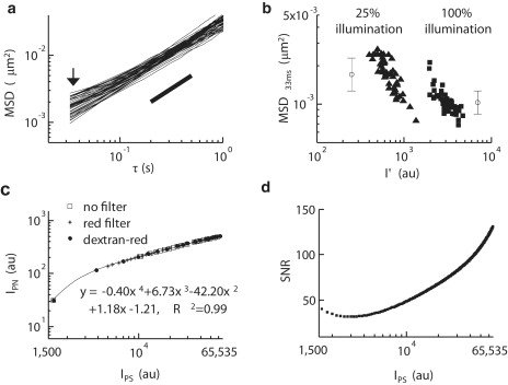
Mean square displacement (MSD) is correlated to the peak intensity (I′) of microspheres tracked by a charge-coupled device (CCD) camera. (a) A MSD versus time lag plot of microspheres (n = 47) embedded in glycerol shows the presence of MSD variation in a homogeneous aqueous solution (arrowhead). The particle-tracking experiments were conducted at a time resolution of 33 ms with using 25% of full power of illumination. (b) A logarithm plot of MSD (τ = 33 ms) versus peak intensity of microspheres (n= 53) embedded in glycerol under 25% (▴) and 100% (■) power of illumination suggests a relationship between increasing peak intensity and decreasing MSD value. The error bar shows the mean and standard deviation of the MSD (τ = 33 ms). (c) Digital intensity signal (I_PS) and noise (I_PN) values are extracted from uniform light sources: the head light without a filter (open squares), the head light with a red filter (+), and the ultraviolet-visible light with a red filter at different concentration of rhodamine B-tagged 70 kD Dextran (solid circles). The I_PS-I_PN relationship is expressed by a fourth-order polynomial fit. (d) Signal/noise ratio (SNR) versus digital signal intensity may be determined by the curve fitting described in panel c to well-estimate the SNR as a function of the digital signal strength ranging between saturated signal (65,535 arbitrary units (au)) and dark current (∼1500 au).

In the preceding function, StoN represents the empirically measured correlation between I_PS and I_PN (in the case herein, it is a fourth-order polynomial; see Fig. 1 c). R(0,1) represents a normally distributed random number with zero mean and unit variance. Here a Gaussian noise was used to represent the system noise over the full-intensity spectrum. The noise sources in a pixel of CCD are mainly dominated by readout and photon shot noise. The noise intensity histogram of the CCD camera of the experimental system displayed a Gaussian distribution throughout the entire CCD signal sensing range from 1300 arbitrary units (au) to 65,535 au. The R-squared value from fitting a Gaussian distribution to the entire spectrum of I_PS in the experiment was always higher than 0.98, suggesting that the use of a Gaussian random number in the Monte Carlo simulation to represent I_PS could be justified. This is in agreement with previous independent studies, which demonstrated that the combined noises, including shot noise, dark noise, and readout noise, show a Gaussian distribution for a high influx of photons (13,17).

The simulated image was further processed through the particle-tracking algorithm to estimate the simulated particle's position. Six hundred trials were tested for each condition to estimate the uncertainty in positioning and the relative error for this estimation was found to be below 3%. The position error (ɛ_p) is defined as the distance between the true position and the position estimated by the tracking algorithm. Spatial resolution (ɛ), and hence static error (2ɛ²), is estimated from the summation of standard deviation in the x and y directions.

Rheometer

Conventional rheology studies on the glycerol samples were conducted using an AR-G2 stress-controlled software-operated rheometer (TA Instruments, New Castle, DE). Glycerol was loaded into a 60-mm cone-and-plate sampler module (cone angle = 1°). To determine the viscoelastic properties of a glycerol, the sample was subjected to 0.05% sinusoidal shear strains with the frequency gradually increasing from 0.01 to 50 Hz (frequency sweep test) under isothermal conditions (23°C).

Intracellular particle tracking and cytoplasmic rheology

MC3T3-E1 (Riken Cell Bank, Tokyo, Japan) were cultured in αMEM supplemented with 10% fetal bovine serum (Hyclone, Logan, UT), 100 IU/ml penicillin, and 100 μg/ml streptomycin and maintained at 37°C in a humidified, 5% CO₂ environment. Cells were passed every 3–4 days and seeded (∼1 × 10⁴ cells/ml) onto 10-cm cell culture dishes. Before particle-tracking experiments, MC3T3-E1 cells were plated on 35-mm cell culture dishes and subjected to ballistic injection of 100-nm carboxylated polystyrene fluorophores (Invitrogen) using a Biolistic PDS-1000/HE particle-delivery system (Bio-Rad, Hercules, CA). In the ballistic injection process, nanoparticles were placed on macrocarriers and allowed to dry for 2 h. Rupture disk with 1800-psi rupture pressure were used in conjunction with a hepta adaptor (3). After injection, cells were plated again using αMEM supplemented with 5% fetal bovine serum on dishes coated with 20 μg/ml fibronectin (EMD Chemicals, Gibbstown, NJ). Culture medium was replaced the next day with serum-free αMEM. Cells were serum-starved for 48 h before the particle-tracking experiments.

After the particle-tracking experiment, the MSD of each probe nanosphere was directly related to the local creep compliance (18) of the cytoplasm, Γ(τ), as

$$\mathrm{\Gamma }\left(\tau \right)=\frac{3\pi a}{2k_{\mathrm{B}}T}\langle \mathrm{\Delta }{r}^2\left(\tau \right)\rangle \text{.}$$ (6)

The creep compliance (expressed in units of cm²/dyne, the inverse of a modulus) describes the local deformation of the cytoplasm induced by the thermally excited displacements of the nanoparticles. If the cytoplasm around a nanosphere behaves as fluid-like (e.g., glycerol), then the creep compliance increases continuously and linearly with time, with a slope that is inversely proportional to the shear viscosity, Γ(τ) = τ/η. If the cytoplasm behaves locally as solid-like (e.g., a gel), then the creep compliance is a constant with a value inversely proportional to the elasticity of the gel, Γ(τ) = 1/G₀. The local frequency-dependent viscoelastic parameters of the cytoplasm, G′(ω) and G″(ω) (both expressed in units of dyn/cm², a force-per-unit area), were computed in a straightforward manner from the MSD (4). The elastic modulus, G′, and viscous modulus, G″, describe the propensity of a complex fluid to resist elastically and to flow under mechanical stress, respectively.

Results

Light source affects the MSD values

The consistency of a purely homogeneous medium should be reflected by an identical MSD value for each tracked particle at any given time lag. This was not observed for glycerol, which had a distribution of MSDs inconsistent with a homogeneous medium, especially at shorter time lags (Fig. 1 a). Analysis of this discrepancy revealed a correlation between MSD (τ = 33 ms) and the peak intensity for individual microspheres (Fig. 1 b). Emission outside of the microscope's focal plane or interference from other randomly distributed particles obstructing the light path may affect the light intensity emitted from a microsphere to the photon detector, causing a distribution of peak intensity within a sample. Additionally, the digitization of photon signals by the detector introduces shot noise, and may also involve other types of noise (17). The presence of this combined noise could introduce significant bias in image analysis, making it essential to correct MSD values in particle-tracking experiments.

Subsequently, it was investigated whether the error revealed by the variation in MSD directly stems from the intensity fluctuations of the overall recorded signal. This was accomplished by extracting the signal and noise information from individual pixels throughout the whole image. Different pixels do not generate purely random noise under the same projected light due to noise inherent to the measurement device such as dark current variation and fixed pattern noise (17), which are consistently associated with an individual pixel and independent of outside signals. To eliminate this bias from each pixel, one reference image was set as a standard, and a successive image with the same illumination was then subtracted from the reference image (17). This procedure resulted in an even-weight (one bit of data per pixel) array with nonbiased random noise. The random noise had an approximate Gaussian distribution and zero mean (consistently biased noise and the background intensity are filtered by the reference image subtraction). Therefore, the intensity of homogeneous light emitted from a halogen bulb can be determined by the mean pixel intensity (I_PS) for pixels over the whole image, and a distribution profile of random noise corresponding to the illumination source can be determined to obtain the mean random noise intensity (I_PN) (see Materials and Methods).

Using the above method, images of water were taken under a homogeneous field of collimated light from a halogen bulb, either with or without a 590-nm cut-off (red) filter in the light path, or with various concentrations of rhodamine B-labeled dextran with a red filter, to extract the I_PS and the I_PN particular to the microscope being used. Using a CCD camera, a consistent correlation between I_PS and I_PN emerged from each of the three different experimental settings, over the full working range of light intensity (Fig. 1 c). Therefore, the correlation between I_PS and I_PN suggests that a tracking system could possess a digital output signal dependent noise, which cannot be simply expressed by only shot noise (I_PN = I_PS^1/2) (14), Gaussian noise (I_PN = N, where N is a constant) (12), nor a combination of both (I_PN = I_PS^1/2 + N) (13).

Consequently, this information was used to effectively estimate the SNR (I_PS/I_PN) for pixels over the full spectrum of I_PS (Fig. 1 d). These data further revealed that varying light intensity drastically affects the SNR for the camera readout, with brighter particles yielding better spatial resolutions. Furthermore, because the settings of a CCD camera (such as the gain in on-chip multiplication) can alter the correlation between I_PS and I_PN, the method demonstrated here offers a generic procedure to easily extract the SNR profile from any CCD camera-based tracking system for static error determination.

Interplay of several factors determines the static error

The SNR determined for the tracking system was then applied to create simulated images, which were used as a basis for investigating the conditions governing I_PS fluctuations and the degree of particle positioning bias. A Gaussian-shaped simulated bead was constructed (see Materials and Methods), which had a defined peak intensity (I), radius (R_a) and subpixel location (μ_x = μ_y = 0 for the center of the pixel), with a homogeneous background intensity (I_B). Once the bead parameters were assigned, the appropriate level of random noise was added to individual pixels in the simulated image based on the established SNR (Fig. 1 d). Subsequently, the simulated image containing the “system-noise” was added to the particle-tracking algorithm to determine the “experimental” tracked position of the bead. These images were reconstructed multiple times to represent separate tracking trials under the given initial parameters, and the spatial resolution (i.e., standard deviation of the positioning distribution) of the bead was obtained after conducting a statistically meaningful number of such trials (Fig. 2 a).

Figure 2.

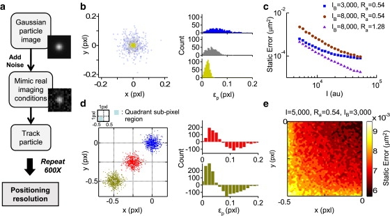
Static error (2ɛ²) can be estimated using simulated Gaussian beads. (a) A flow diagram demonstrates how to estimate static error by Monte Carlo simulation. (b) Distribution patterns of tracked positions were generated by running 600 independent trials incorporating pixel noise into simulated images using three different intensities of Gaussian beads (I = 5000 (blue), 10,000 (gray), and 50,000 (yellow)) with μ_x = μ_y = 0, R_a = 0.54, and I_B = 3000 (left panel). Three histograms in the right panel indicate the distribution of the experimental position error, ɛ_p (the displacement between the experimental center and the assigned center). Beads possessing a higher intensity generate smaller experimental errors with sharper distributions. (c) Static error versus the assigned peak intensity (I) is plotted for the three different Gaussian beads. (d) Left: The distribution of the tracked center after 600 simulations for Gaussian beads initially in three subpixel locations within the lower-left pixel quadrant ((0, 0), (−0.25, −0.25) and (−0.5, −0.5)) is shown. Right: A histogram of 6000 positioning error simulations for Gaussian beads located at the pixel center was set as a reference for off-center beads, and differences in count of the tracked displacements suggest that the subpixel location of a microsphere affects the size of its positioning error. (e) The intensity diagram illustrates the correlation between static error and the Gaussian particle subpixel location at a resolution of 0.01 pixels. The intensity bar indicates the range of static error.

Using this Monte Carlo approach, an investigation was conducted of the relationship between the peak intensity of particles (I) and the resulting positioning distributions. Trials for three different Gaussian bead peak intensities (μ_x = μ_y = 0, R_a = 0.54 and I = 5000, 10,000, and 50,000, respectively) with a uniform background intensity (I_B = 3000) suggested that the positioning error is related to the peak intensities (Fig. 2 b, left). In addition, the brighter peak intensities resulted in a tighter distribution of tracked positions and a smaller positioning error (Fig. 2 b, right). Because the spatial resolution (ɛ) can be quantitatively linked to the static error (2ɛ²) (12–14), the brighter peak intensities directly translate to a diminished static error. Moreover, static error versus the peak intensity was plotted for Gaussian beads having three sets of I_B and R_a values to demonstrate the dependence of static error on these additional parameters (Fig. 2 c). In each case, the static error always decreased incrementally with Gaussian bead peak intensity.

The final Gaussian bead parameter that could have an effect on the static error profile was the subpixel location. Under a uniform I_B, Gaussian beads with a fixed I and R_a were assigned different subpixel locations, i.e., (μ_x, μ_y) = (0, 0), (−0.25, −0.25), and (−0.5, −0.5), where μ_i = 0 corresponded to the pixel center and μ_i = −0.5 corresponded to the pixel edge, respectively. The static error extracted from the set centered within the pixel was used as a reference to observe deviations in the error distribution at other bead locations. Monte Carlo simulations suggested a trend of increasing error as Gaussian beads move closer to the pixel edge (Fig. 2 d). To further understand this trend, the evaluation of subpixelation effects on the static error was repeated throughout a whole pixel quadrant (because there is symmetry about the pixel center in both the x- and y-axis). It was found that the subpixel position can augment static error up to 1.5-fold (from ∼6 × 10⁻³ μm² to ∼9 × 10⁻³ μm²) for a single set of assigned bead parameters (Fig. 2 e). Thus, the subpixel localization of the bead center also contributes to the static error, revealing that several bead parameters collectively contribute to the propagation of such error.

Direct parameter mapping can be used to accurately estimate the static error

Although the static error extracted from the Monte Carlo trials is affected by the individual manipulation of peak intensity, radius, subpixel location, and background intensity values, these parameters may not be independent or constant throughout an actual experiment. As particles move out from the focal plane, their projected image will simultaneously appear to have a larger radius and a dimmer peak intensity than if they were in focus (19). The background intensity also changes for different microscopic and environmental conditions. Furthermore, some microenvironments constrain particles so that the total displacement of a particle during short lag times can be less than the pixel size (i.e., a particle embedded in highly viscous and/or highly elastic media). In this case, subpixel localization of the particle will be a dominant factor for static error in the tracking analysis. Therefore, the accurate representation of experimental particles necessitates a case-by-case assignment of the proper Gaussian bead parameters to validate the Monte Carlo approach of extracting the spatial resolution using simulated images.

Particle-tracking algorithms independently process microspheres in the acquired images and produce a set of experimental parameters, (R_a′, I′, μ_x′, and μ_y′) to describe each tracked microsphere. However, these parameters cannot represent the true characteristics of particles because they have been processed by convolution of the tracking algorithm, and cannot be directly used to extract the static error by Monte Carlo simulation. A mapping procedure has been developed to estimate the true parameters (R_a, I, μ_x, and μ_y) of the original microsphere from the convolved images of the nonlinear algorithm tracking analysis (Fig. 3 a). During this process, the addition of extracted system noise to the simulated images was omitted to avoid generating additional variation in the image data that would only corrupt the comparisons.

Figure 3.

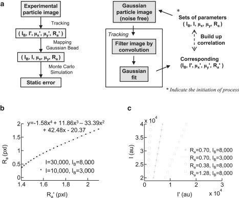
Method to relate extracted static error from simulated beads to experimental microsphere images is demonstrated. (a) The left flow chart demonstrates the process of estimating static error from raw particle image. The process retrieves tracked parameters from a raw image, maps the adequate parameters to simulate experimental images with the complementary Gaussian particle, and applies Monte Carlo simulation to estimate the static error. The right flow chart shows the procedure used to map parameters for simulated Gaussian beads to match experimental tracked parameters. (b) A fourth-order polynomial equation can be adopted to describe the relationship between the radius of the simulated Gaussian bead, R_a, and the radius of tracked microsphere, R_a′, with perfect fitting (R² = 1). This result is independent of the peak intensity, I, and background intensity, I_B. (c) The Gaussian bead peak intensity (I) versus the experimental peak intensity (I′), plotted for three different Gaussian bead radii, showing a linear correlation between I and I′. The plot also suggests that the correlation is independent of the pixel background because lines are overlaid at the same R_a despite having pixel backgrounds that are set differently.

The mapping begins by assuming that the absolute position of a simulated Gaussian bead, (μ_x, μ_y), is the same as the experimentally tracked positions, (μ_x′, μ_y′). This assumption has previously been evaluated with the conclusion that the pixilization effects can only generate up to 0.02 pixels of error (12). Several simulated Gaussian bead images generated by a series of R_a values (from 0.38 to 1.80 pixels), and different peak and background intensities were subjected to the tracking algorithm to retrieve the corresponding apparent radii (R_a′). A scatter plot of R_a to R_a′ fit by a fourth-order polynomial with perfect regression (R² = 1) (Fig. 3 b) is evidence that the correlation of R_a and R_a′ depends only on the tracking algorithm and is independent of the peak intensity of the Gaussian bead and the background pixel intensity. Having accounted for all other Gaussian bead parameters, the relationship between I and I′ was uncovered using a linear curve fitting (Fig. 3 c). The entire mapping procedure was repeated for a range of Gaussian bead parameter configurations until a clear link between simulated and experimental tracking images was evident. Through this simple process, any typical microsphere experimental image can be precisely simulated by a corresponding Gaussian bead image (Fig. 4). The mapped values of the pixel intensity in a 3 × 3 pixel region are comparable between the simulated bead and the experimentally tracked microsphere. This result demonstrates that the correlations determined by our procedure can be used to define experimentally relevant Gaussian beads to determine static error.

Figure 4.

Gaussian bead with the parameters determined by the mapping procedure in this article can represent the experimental microsphere. The experimental (left) and simulated (right) data are in agreement, as evident in their images and the pixel intensity of the 3 × 3 area surrounding the brightest pixel.

Procedure verification using in vitro and in situ experimental systems

The accuracy of the mapping procedure was verified by imaging static particles. Several microspheres were immobilized onto a coverslip and their MSDs were tracked. Immobilized microspheres should exhibit approximately no movement, and the detected MSD values are expected to represent the static error. The mapping procedure was applied to estimate the static error from the experimental images. Comparing the experimental static error of each microsphere to its peak intensity revealed that static error invariably reduces when the peak intensity of the corresponding microsphere increases (Fig. 5 a). Using the Monte Carlo simulation trials, the static error (2ɛ²) was extracted and correlated to the experimental static error in a log-log plot showing that the simulated static error is in agreement with the experimental results (MSD), having a strong linear correlation (R² = 0.99) (Fig. 5 b). This strong correlation confirms that the Monte Carlo simulation approach explained herein can successfully estimate real-time static error.

Figure 5.

Static error can be corrected for the MSD of microspheres embedded in glycerol. (a) A sample of fixed microspheres is used to verify the estimated static error from simulations by representing the tracked MSD values as the spatial error generated from the experimental system. In a logarithm scale, the individual microsphere's peak intensity is inversely proportional to its MSD (the approximate experimental static error). (b) The logarithm of experimental static error (MSD at 33 ms) and the corresponding estimated simulated static error strongly correlate with a linear fit, R² = 0.99. (c) Raw MSD data from particle tracking under 25% power of illumination (n = 47) exhibits a degree of heterogeneity in the data, but raw MSD data (n = 53) and its corrected MSD both obtained under 100% power of illumination share a similar scale and trend as the corrected MSD from low illumination (25%). (d) The mean viscous modulus, G″, of glycerol is estimated at time lags of 33 ms from the raw and corrected MSD values at 25% and 100% power of illumination, respectively. The dashed line indicates the viscous modulus measured by a conventional rheometer, and the star denotes the significantly lower G″ of the raw MSD at 25% power of illumination using a two-tailed t-tests with p < 0.05. (e) The illustration explains how errors generated from the experimental system can affect the MSD result in the cases of glycerol: measured MSD is the culmination of system MSD and static error.

MSD data from a standard tracking analysis in glycerol was corrected using this technique by directly subtracting the estimated static error value. Comparison between the raw and corrected results under low (25%) and high (100%) illumination suggests that the correction produce significantly more precise results, reflecting the true nature of the homogeneous Newtonian fluid (Fig. 5 c). When the generalized Stokes-Einstein Relation was used to convert the MSDs to the viscous modulus, it was found that the values are underestimated in the raw MSDs of low illumination, but are accurate when the MSDs are calibrated or are obtained from high-illumination experiments (Fig. 5 d). This provides another validation of the fact that static error is important in tracking experiments and should be eliminated using the correction algorithm (Fig. 5 e).

Further investigations demonstrated the use of the correction technique for tracking particles inside cells and calculating the creep compliance from the MSD data. One-hundred-nm diameter, carboxylated fluorescent microspheres were ballistically bombarded into the cytoplasm of a MC3T3-E1 fibroblasts culture. After serum-starving for 48 h, the majority of particles were evenly distributed into the cytoplasmic region of the cells (Fig. 6 a). In comparison with a standard cell culture, serum-starved cells lack massive actin-cytoskeletal structures in most of their cytoplasmic region (20), and in this cytoskeletally depleted zone, particles are permitted to exhibit a relatively greater degree of free diffusion. Yet, the timescaling profile of the raw MSDs obtained from particle tracking indicate that almost all such particles in the cytoplasmic region move subdiffusively (Fig. 6 b). In contrast, the corrected MSD values obtained by the approach herein suggest that these particles are less subdiffusive (Fig. 6 c). This analysis strongly advocates the necessity of eliminating static error from MSD measurements for correctly probing the cellular biophysical properties using particle tracking.

Figure 6.

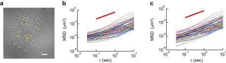
Static error can be corrected for the MSD of 100-nm carboxylated polystyrene particles embedded in MC3T3-E1 fibroblast cells under red-fluorescence. (a) An image acquired from our CCD camera. Square dots indicate the positions of microspheres within the frame. (b) A MSD versus time lag plot extracted from the cellular system (80 particles in seven cells) implies subdiffusive particle motion at shorter lag times, indicating a range of local microenvironments that the microspheres are encountering. (c) Using our method to subtract out the estimated static error in the system revealed a new MSD profile, which implies more diffusive particle motion throughout the cellular environment at short lag times.

Discussion

MSD inaccuracy due to static error is ubiquitous in CCD camera-based particle-tracking systems. However, the complex interplay between multiple tracking parameters had precluded the development of a practical method to minimize the errors. The correction approach explained herein significantly minimizes static error. This approach circumvents the complication of direct static error calculation by employing a simulation-based method to correct experimental particle-tracking measurements. This considerably enhances the accuracy of the MSD and improves the subsequent estimation of diffusivity as well as rheological properties.

Tracking of particles in a homogenous glycerol solution resulted in a wider MSD distribution at short lag times with decreasing light source intensity. This result indicates that static error can significantly bias the MSD profile, potentially causing a misinterpretation of the underlying physical properties (11). Static error in the tracking system used herein can be estimated to be between ∼2 × 10⁻⁵ μm² and ∼10⁻³ μm² by tracking immobilized microspheres, suggesting that measured MSD values within this range are clearly unreliable. However, elimination of this static error allows for an accurate MSD measurement with a resolution of ∼10⁻⁶ μm² from a sufficiently bright particle.

In the simulation approach, the simulated Gaussian bead has a single “point” position expressing the peak intensity, which is an appropriate model to match with the Gaussian fit algorithm. The particle diameter used in this study was 100 nm, whereas many in vitro studies have applied particles of a larger size for tracking. Compared to larger particles, the 100-nm particle is more suitable to be considered as a “point” light source. Meanwhile, a previous study (P.-H. Wu, and Y. Tseng, unpublished data) suggested that the estimated static error is comparable to the measured MSD obtained from fixed 1-μm particles. In essence, this method can be applied to the current particle-tracking experiments regardless of the particle size.

However, there are some additional advantages to the use of 100-nm particles that were chosen for this work. Light scattering by tracking particles can directly affect the background signal in a tracking video while simultaneously depleting the detectable peak intensity within the exposure time. These effects can have a detrimental outcome on the proper estimation of MSD. Based on the Mie theory, the main parameter to consider in elastic light scattering is the size parameter, x = 2πR/ λ, where λ is the wavelength and R is the radius of the particle. The wavelength of the light used in the video-based particle-tracking experiment ranges between ∼400 and 700 nm. Therefore, the 100-nm size particle has an x ∼ 0.5, in which the extinction coefficient is negligible and light scattering effects are minimized. Meanwhile, Rayleigh scattering will not affect the particle-tracking results unless the size of the particle is reduced to ∼10 nm.

For a 1-μm particle, the size parameter of light scattering is approximately equal to 5, and the extinction coefficient approaches the maximum value. Therefore, light absorbance by 1-μm particles is inevitable. Nevertheless, the emitted signal from a 1-μm particle is much higher than the detectable threshold (SNR is much greater compared to the 100-nm particle). The larger particle should have much smaller static error. However, when the particle size increases from 100 nm, the extinction coefficient consequently increases as well, which would generate heat and increase the temperature to the microenvironment. Therefore, heat effects on the experiments would need to be assessed.

To ensure that the discrepancy of MSD values of 100-nm particles embedded in glycerol was not an effect of heat generated from different power settings of the light source, particle tracking was repeated successively three times on a sample at full power of light intensity. In this case, the sample was exposed to constant light for more than 1 min. The three tracking results were carefully compared to evaluate whether the MSD values shift toward higher or lower values. The result showed that there was no heat accumulation, which would affect a change in the MSD (data not shown). The short lag-time MSD values for the first 5-s period and the last 5-s period in the same experiment were also evaluated to examine the transient heat build-up, and it was concluded that the difference of MSD values were not caused by the heat effect for the 100-nm particles.

In summary, this correction technique is not limited to the particular system used herein, but is broadly applicable to any tracking system. The transition to another system requires simple steps of determining the correlation between the pixel signal and noise, and appropriately selecting correct tracking parameters. By closely following the methodology described herein, static error can be significantly eliminated, leading to a greater clarity when interpreting the MSD values from a particle-tracking experiment.

References

- 1.Wieser S., Moertelmaier M., Fuertbauer E., Stockinger H., Schutz G.J. (Un)confined diffusion of CD59 in the plasma membrane determined by high-resolution single molecule microscopy. Biophys. J. 2007;92:3719–3728. doi: 10.1529/biophysj.106.095398. [DOI] [PMC free article] [PubMed] [Google Scholar]
- 2.Saxton M.J., Jacobson K. Single-particle tracking: applications to membrane dynamics. Annu. Rev. Biophys. Biomol. Struct. 1997;26:373–399. doi: 10.1146/annurev.biophys.26.1.373. [DOI] [PubMed] [Google Scholar]
- 3.Lee J.S.H., Panorchan P., Hale C.M., Khatau S.B., Kole T.P. Ballistic intracellular nanorheology reveals ROCK-hard cytoplasmic stiffening response to fluid flow. J. Cell Sci. 2006;119:1760–1768. doi: 10.1242/jcs.02899. [DOI] [PubMed] [Google Scholar]
- 4.Kole T.P., Tseng Y., Huang L., Katz J.L., Wirtz D. Rho kinase regulates the intracellular micromechanical response of adherent cells to rho activation. Mol. Biol. Cell. 2004;15:3475–3484. doi: 10.1091/mbc.E04-03-0218. [DOI] [PMC free article] [PubMed] [Google Scholar]
- 5.Gorisch S.M., Wachsmuth M., Ittrich C., Bacher C.P., Rippe K. Nuclear body movement is determined by chromatin accessibility and dynamics. Proc. Natl. Acad. Sci. USA. 2004;101:13221–13226. doi: 10.1073/pnas.0402958101. [DOI] [PMC free article] [PubMed] [Google Scholar]
- 6.Jin S., Haggie P.M., Verkman A.S. Single-particle tracking of membrane protein diffusion in a potential: Simulation, detection, and application to confined diffusion of CFTR Cl- channels. Biophys. J. 2007;93:1079–1088. doi: 10.1529/biophysj.106.102244. [DOI] [PMC free article] [PubMed] [Google Scholar]
- 7.Cabal G.G., Genovesio A., Rodriguez-Navarro S., Zimmer C., Gadal O. SAGA interacting factors confine sub-diffusion of transcribed genes to the nuclear envelope. Nature. 2006;441:770–773. doi: 10.1038/nature04752. [DOI] [PubMed] [Google Scholar]
- 8.Apgar J., Tseng Y., Fedorov E., Herwig M.B., Almo S.C. Multiple-particle tracking measurements of heterogeneities in solutions of actin filaments and actin bundles. Biophys. J. 2000;79:1095–1106. doi: 10.1016/S0006-3495(00)76363-6. [DOI] [PMC free article] [PubMed] [Google Scholar]
- 9.Borgdorff A.J., Choquet D. Regulation of AMPA receptor lateral movements. Nature. 2002;417:649–653. doi: 10.1038/nature00780. [DOI] [PubMed] [Google Scholar]
- 10.Haft D., Edidin M. Cell biology - modes of particle-transport. Nature. 1989;340:262–263. [Google Scholar]
- 11.Martin D.S., Forstner M.B., Kas J.A. Apparent subdiffusion inherent to single particle tracking. Biophys. J. 2002;83:2109–2117. doi: 10.1016/S0006-3495(02)73971-4. [DOI] [PMC free article] [PubMed] [Google Scholar]
- 12.Savin T., Doyle P.S. Static and dynamic errors in particle tracking microrheology. Biophys. J. 2005;88:623–638. doi: 10.1529/biophysj.104.042457. [DOI] [PMC free article] [PubMed] [Google Scholar]
- 13.Thompson R.E., Larson D.R., Webb W.W. Precise nanometer localization analysis for individual fluorescent probes. Biophys. J. 2002;82:2775–2783. doi: 10.1016/S0006-3495(02)75618-X. [DOI] [PMC free article] [PubMed] [Google Scholar]
- 14.Cheezum M.K., Walker W.F., Guilford W.H. Quantitative comparison of algorithms for tracking single fluorescent particles. Biophys. J. 2001;81:2378–2388. doi: 10.1016/S0006-3495(01)75884-5. [DOI] [PMC free article] [PubMed] [Google Scholar]
- 15.Gonzalez R.C., Woods R.E. Prentice Hall; Upper Saddle River, NJ: 2002. Digital Image Processing. [Google Scholar]
- 16.Hong Q.A., Sheetz M.P., Elson E.L. Single-particle tracking - analysis of diffusion and flow in 2-dimensional systems. Biophys. J. 1991;60:910–921. doi: 10.1016/S0006-3495(91)82125-7. [DOI] [PMC free article] [PubMed] [Google Scholar]
- 17.Reibel Y., Jung M., Bouhifd M., Cunin B., Draman C. CCD or CMOS camera noise characterisation. Eur. Phys. J. Appl. Phys. 2003;21:75–80. [Google Scholar]
- 18.Xu J.Y., Viasnoff V., Wirtz D. Compliance of actin filament networks measured by particle-tracking microrheology and diffusing wave spectroscopy. Rheologica Acta. 1998;37:387–398. [Google Scholar]
- 19.Speidel M., Jonas A., Florin E.L. Three-dimensional tracking of fluorescent nanoparticles with subnanometer precision by use of off-focus imaging. Opt. Lett. 2003;28:69–71. doi: 10.1364/ol.28.000069. [DOI] [PubMed] [Google Scholar]
- 20.Kole T.P., Tseng Y., Jiang I., Katz J.L., Wirtz D. Intracellular mechanics of migrating fibroblasts. Mol. Biol. Cell. 2005;16:328–338. doi: 10.1091/mbc.E04-06-0485. [DOI] [PMC free article] [PubMed] [Google Scholar]