

Abstract
Multiphoton fluorescence recovery after photobleaching is a well-established microscopy technique used to measure the diffusion of macromolecules in biological systems. We have developed an improved model of the fluorescence recovery that includes the effects of convective flows within a system. We demonstrate the validity of this two-component diffusion-convection model through in vitro experimentation in systems with known diffusion coefficients and known flow speeds, and show that the diffusion-convection model broadens the applicability of the multiphoton fluorescence recovery after photobleaching technique by enabling accurate determination of the diffusion coefficient, even when significant flows are present. Additionally, we find that this model allows for simultaneous measurement of the flow speed in certain regimes. Finally, we demonstrate the effectiveness of the diffusion-convection model in vivo by measuring the diffusion coefficient and flow speed within tumor vessels of 4T1 murine mammary adenocarcinomas implanted in the dorsal skinfold chamber.
Introduction
Fluorescence recovery after photobleaching (FRAP) was developed in the 1970s as a method to probe the local mobility of macromolecules in living tissue (1–4). Briefly, FRAP is performed by using an intense laser flash to irreversibly photobleach a region of interest within a fluorescent sample and then monitoring the region of interest with the attenuated beam as still-fluorescent molecules from outside the region diffuse inward to replace the bleached molecules. FRAP relies on single-photon excitation of the fluorescent sample, which generates fluorescence throughout the light cone of the objective. Fluorescence and photobleaching are therefore unconfined in three dimensions, generally limiting the technique to thin samples (∼1 μm) for measurement of absolute diffusion coefficients. FRAP with spatial Fourier analysis (5,6) allows thicker samples to be investigated; however, deep-tissue imaging is still prohibited due to the poor depth penetration of epifluorescence microscopy. The FRAP technique was significantly enhanced with the advance to multiphoton excitation. The intrinsic spatial confinement of multiphoton excitation (7) allows multiphoton fluorescence recovery after photobleaching (MP-FRAP) to be performed within thick samples, while the greater depth penetration of multiphoton imaging (8) allows MP-FRAP to be performed deep within scattering samples (9).
The existing mathematical theory of MP-FRAP assumes that diffusion is the only recovery mechanism and so does not account for the possibility of convective flow within the focal volume, a situation that is now likely to arise as MP-FRAP is applied to a greater variety of in vivo applications. The presence of an unexpected significant convective flow in an MP-FRAP experiment can produce erroneously high diffusion coefficients when the existing diffusion-only model is used to analyze the data. It is important, therefore, to include convective flow in the MP-FRAP derivation and to determine over what range of flow speeds the MP-FRAP technique can thereby provide accurate diffusion coefficients.
We expect this new diffusion-convection model to be crucial for diffusion studies conducted in tissues with above-average interstitial flow. Kidney studies, for example, are already enjoying advances due to the application of multiphoton imaging techniques (10–12). Interstitial flow within the juxtaglomerular apparatus of the kidney has been measured via multiphoton video imaging to be 27.9 ± 7.2 μm/s (13), which is a significant enough flow speed to elicit erroneous diffusion coefficients when measured via MP-FRAP and fit to the diffusion-only model. MP-FRAP with the new derivation may also find a place in the burgeoning world of microfluidics, where measurements of diffusion coefficients (and flow speeds) are already in demand (14–16).
Through application of the Stokes-Einstein relation, the diffusion coefficient obtained from MP-FRAP measurements can be used to calculate fluid viscosity. In a healthy human, blood plasma viscosity maintains a narrow range of values, 1.10–1.30 mPas at 37°C (17). An elevated plasma viscosity, in the extreme case (greater than twice the normal value) known as hyperviscosity syndrome (18), is indicative of many disease states. For example, a positive correlation has been found between the degree of plasma viscosity elevation and the severity of coronary heart disease (19), as well as the incidence of heart attack or stroke (20–22). Hyperviscosity is often associated with Waldenström's macroglobulinemia and multiple myeloma (23). Elevated plasma viscosity has been indicated in cancer development, particularly among the gynecologic cancers (24). Plasma viscosity can also be used to assess changes in acute phase response due to trauma (17,25). MP-FRAP offers a noninvasive, real-time measure of plasma viscosity, which could be used to probe more deeply the connection between plasma viscosity and these (and other) disease states and/or the response of these disease states to treatments. However, our results show that measurement of the diffusion coefficient, and therefore plasma viscosity, in blood vessels requires the use of our diffusion-convection model for accurate fitting of MP-FRAP recovery curves under the influence of significant directed flow.
A fortunate benefit of the new derivation is that for a relatively wide range of diffusion coefficients and flow speeds, both parameters can be measured accurately. Other techniques have addressed the possibility of combined convective flow and diffusive transport. Axelrod et. al. (2) derived a diffusion-convection model similar to the one presented here, but for conventional (one-photon) FRAP. Later researchers utilized FRAP with Fourier analysis, which uses a video-based analysis of photobleaching recovery data to measure flow speeds and offer insight into flow directions (26–28). Fluorescence correlation spectroscopy is also capable of measuring flow speeds (29), while single particle tracking offers a true velocity vector (30,31).
As discussed, however, single-photon excitation techniques fail to offer the combined spatial resolution and depth penetration of MP-FRAP. Other techniques offering similar spatial resolution as MP-FRAP include multiphoton fluorescence correlation spectroscopy (32,33) and the closely related two-photon image correlation spectroscopy (ICS) (34). Both of these techniques are capable of measuring flow velocities, as well as diffusion, and two relatively new variations of image correlation spectroscopy, k-space ICS (35), and spatio-temporal ICS (36), explicitly offer the ability to measure diffusion coefficients and velocity vectors simultaneously. However, the need of the various correlation spectroscopies for both low concentrations of fluorophores and low background noise, compared with the need of FRAP techniques for high concentrations of fluorophores and subsequent resistance to background noise, means that the correlation spectroscopies and the photobleaching recovery techniques are complementary, not competitive.
In this article, we will first derive the theory of MP-FRAP with both diffusion and convection. Then, we will use computer-generated data to understand how MP-FRAP curves evolve under flow and to predict how the diffusion-only and diffusion-convection MP-FRAP models will fit data with convective flow. Next, we will perform MP-FRAP experimentally using tracers with known diffusion coefficients in situations with known flow speed, and determine specific cutoff speeds that define regimes where the diffusion-only and diffusion-convection models produce accurate diffusion coefficients (and/or flow speeds). Lastly, we will apply the diffusion-convection model in vivo under a range of flow conditions.
Theory
In the existing MP-FRAP model, diffusion is assumed to be the only mechanism for recovery. The diffusive recovery after a brief bleaching pulse is given by Brown et. al (37),
| (1) |
where β is the bleach depth parameter, τD is the characteristic diffusion time, and R is the square of the ratio of the axial to the radial dimensions of the focal volume. The diffusion coefficient is given by D = ωr2/8τD, where ωr is the radial 1/e2 radius of the two-photon focal volume. With only two fitting parameters, β and τD, fits to the fluorescence recovery using the existing model are very robust. In the absence of flow, a three-to-four decade range of seed values for the fitting parameters required by the fitting program will produce convergence to the same, low-residual, fit.
By adding a time-dependent coordinate shift to the standard model of diffusive recovery before its convolution with the excitation laser profile (see Appendix), we arrive at an improved diffusion-convection model that describes fluorescence recovery in the presence of convective flow, as well as diffusion:
| (2) |
In this model, an additional fitting parameter, τv, is introduced, which describes the characteristic recovery time due to convective flow. For one-dimensional flow parallel to the imaging plane, this equation reduces to
| (3) |
The flow speed is easily calculated as v = ωr/τv. This form of the equation readily reduces to that derived by Axelrod et. al. (2) for thin samples with flow measured via one-photon FRAP if the intensity profile is assumed to be two-dimensional (square-root term in denominator disappears). For the purpose of this article, we will focus on the one-dimensional diffusion-convection form (Eq. 3), unless explicitly stated otherwise. This formula produces MP-FRAP recovery curves that are indistinguishable from MP-FRAP recovery curves derived using the diffusion-only formula (Eq. 1) when flow speeds are extremely low. Increasing the flow speed shortens the recovery time and alters the shape of the MP-FRAP recovery curves, eventually producing curves that approach an almost sigmoidal shape at high flow speeds (see Fig. 1).
Figure 1.
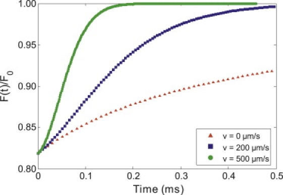
Comparison of the recovery of computer-generated MP-FRAP curves for a macromolecule with D = 9.2 μm2/s and differing values of flow speed. The lower curve is a diffusion-only recovery (v = 0 μm/s), while the middle recovery curve has a moderate amount of flow (v = 120 μm/s), and the upper recovery curve is flow-dominated (v = 500 μm/s). The shape of the curve changes as flow increases, eventually leading to an almost sigmoidal shape for the flow-dominated recovery.
With the improved diffusion-convection model, we can now measure diffusion accurately in the presence of flow while simultaneously measuring the flow speed. However, the introduction of a third fitting parameter complicates the fit. We might now expect that when either diffusion or flow dominates the fluorescence recovery, the fitting program will yield inaccurate values for the nondominant parameter. Care must be taken to define the range of flow speeds over which the diffusion coefficient and flow speed may be measured accurately.
Methods
Computer-generated data and fitting
Fluorescence recovery curves were generated using the diffusion-convection model and fit to both the diffusion-only and diffusion-convection models using the lsqcurvefit function in MATLAB (The MathWorks, Natick, MA). We added Poisson-distributed noise to the generated data in proportion to the relative noise expected for either in vitro (3%) or in vivo (5%) experiments, as determined from previous experience (37). Three experimentally relevant bleach depths were also chosen: 0.2, 0.6, and 1.0 (37). For each bleach depth/noise combination, a range of diffusion coefficients and flow speeds was explored. After fitting the recovery curves, the ratio of fit diffusion coefficient to input diffusion coefficient (with both the diffusion-only and diffusion-convection models) and the ratio of fit speed to input speed (with the diffusion-convection model) were plotted versus input speed. Initial seed values for the fitting parameters required as inputs to the lsqcurvefit function were generated via algorithms developed from limits to the diffusion-convection model equation and assumed no a priori knowledge of the experimental system or of the particular diffusion coefficients and flow speeds. Specifically, the formula used to calculate a seed value for β was derived by solving the recovery equation (Eq. 3) at t = 0 for β in terms of F(0)/Fo, plotting a range of bleach depth parameters as a function of F(0)/Fo, and then choosing the best-fit polynomial to the curve. Seed values for τD were easily estimated as the one-half recovery time of the MP-FRAP recovery curve (τ1/2). And the seed value for flow speed was approximated as v = (x1/2)1/2(ωr/τ1/2), where x1/2 was determined by taking the limit of the recovery equation as , then plotting F(x)/Fo, with x = (vt/ωr)2, and finally picking the value at which F(x)/Fo was half recovered.
Experimental apparatus
Laser light was generated by a tunable, mode-locked Ti:Sapphire laser (Mai Tai; Spectra Physics, Mountain View, CA), yielding 80-fs pulses at a repetition rate of 100 MHz. Rapid modulation of the laser power to produce monitor and bleach intensities was provided by a KDP∗ Pockels Cell (model No. 350-80; Conoptics, Danbury, CT). Timing of the bleach and monitor pulses was delivered by a pulse generator (model No. DG535, Stanford Research Systems, Sunnyvale, CA), while the voltage output to the Pockels Cell was set and switched by a specially designed control box. The output of the Pockels Cell was directed through an Olympus Fluoview 300 laser-scanning microscope to the back aperture of the objective lens (0.8 NA, 40× water immersion; Olympus, Center Valley, PA). Proper overfilling of the back aperture of the objective lens was achieved for all experiments (see PSF Calibration below). Overfilling is accomplished when the 1/e radius of the laser beam is greater than or equal to the radius of the back aperture of the lens. The objective lens focused the excitation beam within the fluorescent sample (Fig. 2). The fluorescence emission was separated from the excitation light by a short-pass dichroic mirror (model No. 670 DCSX-2P, Chroma Technologies, Brattleboro, VT). For the in vitro experiments, emission signals were further separated by a second dichroic mirror and each was detected by a photomultiplier tube (PMT) (Hamamatsu, Bridgewater, NJ). The output from the PMT monitoring the green channel (fluorescent dye; see in vitro MP-FRAP below) could be directed to a photon counter (model No. SR400; Stanford Research Systems, Sunnyvale, CA), for general inquiry into the fluorescence behavior, or to a multichannel scaler/averager (model No. SR430; Stanford Research Systems), for fluorescence recovery data collection. Output from the PMT monitoring the red channel (fluorescent microspheres; see In vitro MP-FRAP below) was directed to the Olympus imaging software. For increased throughput, data collection was largely automated via LabVIEW (National Instruments, Austin, TX).
Figure 2.
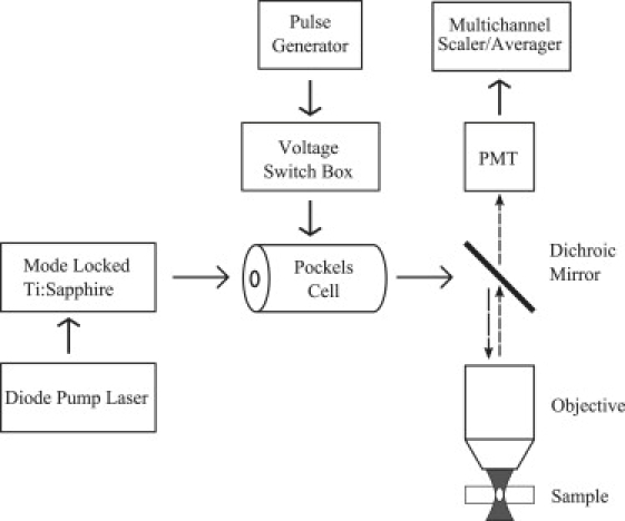
Equipment diagram of MP-FRAP apparatus. To obtain line-scan images for flow speed comparison, a laser scanning system was included in the system. For in vitro experiments, an additional dichroic mirror and PMT were added to separate and measure the red fluorescence of the polystyrene beads.
PSF calibration
The 1/e2 radial and axial dimensions of the two-photon excitation volume were verified by scanning the excitation volume across subresolution fixed fluorescent beads (Molecular Probes/Invitrogen, Eugene, OR). For the radial dimension, xy scans were taken and the intensity profiles of the beads were measured using ImageJ (National Institutes of Health, Bethesda, MD). For the axial dimension, z-stack images were acquired, then the intensity profiles of the beads in each image in the stack analyzed in ImageJ to determine the peaks of the intensity profiles and the peak values plotted versus image depth to build intensity profiles in the axial direction. The results of both measurements were compared against theoretical values. For this work, we defined the 1/e2 radii of the focal volume to be 0.403 μm in the radial direction and 2.22 μm in the axial direction for a 0.8 NA objective, properly overfilled with 780-nm laser light.
In vitro MP-FRAP
For in vitro testing of the flow model, fluorescent samples were produced by mixing fluorescein isothiocyanate (FITC) conjugated to bovine serum albumin (BSA) or 2000 kDa dextran (dextran) (Molecular Probes/Invitrogen) diluted to 1 mg/mL in phosphate buffered saline (PBS) with 1 μL/mL red fluorescent microspheres (FluoSpheres; Molecular Probes/Invitrogen). The solution was suspended in a syringe and allowed to flow freely through a thin tube (0.28 mm radius) and into a channel, capped by a No. 1.5 coverslip and immersed in a pool filled with PBS. The rate of flow was set by adjusting the height of the syringe relative to the channel. For MP-FRAP measurements, the excitation focal volume was kept stationary within the flowing solution in the channel, and the excitation intensity rapidly modulated between a strong bleaching pulse and a weak monitoring pulse. For independent flow speed measurements, the excitation volume was scanned repeatedly along a one-dimensional line parallel to the fluid flow at constant excitation intensity, thus producing a line-scan image with dimensions of position versus time (38). The angle of the sporadic streaks in the line-scan image, representing the movement of the microspheres, was used to calculate the flow speed.
In vivo tumor blood vessel imaging
4T1 murine mammary adenocarcinoma cells (American Type Culture Collection, Manassas, VA) were injected (∼4 × 10⁶ in 50 μL) into the inguinal mammary fat pad of 6–8-week-old female BALB/cByJ mice (Jackson Laboratory, Bar Harbor, ME). Tumors were removed for implant into dorsal skinfold chambers when they reached ∼2.5 mm in diameter.
Male BALB/cByJ mice (Jackson Laboratory) were anesthetized by intraperitoneal injection of a mixture of 90 mg/kg ketamine (IVX Animal Health, St. Joseph, MO) and 9 mg/kg xylazine (Hospira, Lake Forest, IL), and outfitted with a titanium dorsal skinfold chamber as previously described (39). Two days later, a small fragment of 4T1 tumor (∼0.5 mm) was placed in the window of the chamber and allowed to grow for one week before imaging.
Animals containing tumors growing in the dorsal skinfold chamber were anesthetized with ketamine/xylazine, as described above. FITC-dextran was injected intravenously (0.2 mL at 10 mg/mL in PBS), and animals were positioned under the microscope objective lens. MP-FRAP was performed as described above, with the focal volume positioned in the center of the vessel in the xy plane, but largely within the red blood cell-free region along the z axis to maximize fluorescent signal. Line-scans were also performed as described, using the shadows of RBCs, which do not take up FITC-dextran, instead of fluorescent beads.
All animal care and use was in accordance with the policies of the University of Rochester Committee on Animal Resources.
Data analysis
As with the computer-generated data, experimental MP-FRAP recovery curves were fit to the diffusion-only and diffusion-convection models using the MATLAB lsqcurvefit function, which is based on the Levenberg-Marquardt algorithm. Line-scan images were analyzed using ImageJ software.
Results
In silico: testing the limits of the MP-FRAP models
We used computer-generated data to explore the effect of convective flow on the shape and speed of fluorescence recovery, and to probe the conditions (input recovery parameters, noise, focal volume) under which the MATLAB fitting algorithm could correctly recover the diffusion coefficient, assuming the diffusion-convection model is physically accurate (which is tested in In Vitro MP-FRAP). Conditions under which the diffusion-only model produces accurate diffusion coefficients were assessed by generating fluorescence recovery curves using the diffusion-convection model and fitting them to the diffusion-only model, then comparing the input diffusion coefficients and fit diffusion coefficients. Beginning with a combination of a relative noise of 3% and a bleach-depth parameter of 0.6, we generated curves for a series of diffusion coefficients ranging from 0.5 to 500 μm2/s over a range of flow speeds from 0.1 to 10,000 μm/s. Fig. 3 shows that for this series of diffusion coefficients, the diffusion-only model begins yielding erroneously high diffusion coefficients as the flow speed increases, and that the error in determining the diffusion coefficient commences at flow speeds that vary with the diffusion coefficient of the tracer in question. By scaling the speed along the horizontal axis (inset), such that vs = v(ωr/8D), the curves for each value of the diffusion coefficient overlay onto one curve, and a universal behavior can be observed: the diffusion-only model produces erroneous diffusion coefficients () as the scaled speed approaches vs ∼0.3. This scaling behavior allowed us to complete our investigations of the remaining noise/bleach depth parameter combinations using only the diffusion coefficients representative of BSA and dextran, the two tracer molecules used in our in vitro experiments. With all combinations of noise and bleach-depth evaluated (3% and 5% relative noise, and β of 0.2, 0.6, 1.0), we find that the behavior of the Dfit/Dinput curve is unchanged (data not shown). The behavior of the Dfit/Dinput curve also remained unchanged when a significantly larger focal volume was assumed, ωr = 0.646 μm and ωz = 5.81 μm, corresponding to a numerical aperture of 0.5 (data not shown).
Figure 3.
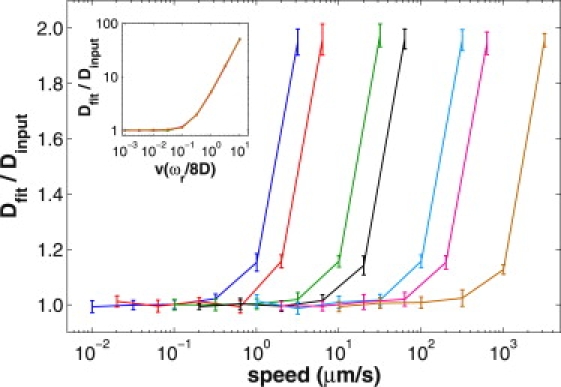
Conditions for accurate fitting using the diffusion-only model, as assessed by fitting computer-generated data. Fluorescence recovery curves were generated with the diffusion-convection model, keeping the bleach depth parameter and relative noise constant at 0.6 and 3%, respectively, while exploring a range of speeds (plotted logarithmically) for each of a set of diffusion coefficients (left to right: D = 0.5, 1, 5, 10, 50, 100, 500 μm2/s). The data were fit to the diffusion-only model, and the diffusion coefficients produced were normalized to the associated input diffusion coefficients. Hence, an accurate result produces a ratio of one. As the input speed increases beyond a certain cutoff value, the diffusion-only model yields a growing overestimate to the diffusion coefficient. By scaling the input speed along the horizontal axis (inset), the curves for each value of the diffusion coefficient overlay onto a single curve.
To evaluate the conditions under which the diffusion-convection model produces accurate diffusion coefficients, we generated, and fit, fluorescence recovery curves using the diffusion-convection model for diffusion coefficients representing BSA and dextran over a range of flow speeds. We show representative results in Fig. 4 a for β = 0.6 and relative noise = 3%, where the ratio of fit diffusion coefficient to input diffusion coefficient is displayed along with the ratio of fit speed to input speed. Of greatest importance to note is that the diffusion-convection model produces accurate values for the diffusion coefficient for values of flow speed much greater than those for which the diffusion-only model produces accurate values for the diffusion coefficient. We also note that at the extremes of the plot, representing results from fits to fluorescence recoveries dominated by either diffusion (on the left) or flow (on the right), the fit accurately determines the dominant parameter (i.e., a ratio of one with a small standard deviation), while poorly determining the nondominant parameter (i.e., a ratio not equal to one and/or a large standard deviation). For a wide range of scaled speeds, the effects of diffusion and flow on the fluorescence recovery dynamics are reasonably balanced, and both the diffusion coefficient and the flow speed are accurately determined. Based on this result, we can define three regimes: 1) diffusion-dominated, in which only the diffusion coefficient is accurately determined; 2) balanced, in which both the diffusion coefficient and flow speed are accurately determined; and 3) flow-dominated, in which only the flow speed is accurately determined. After completing investigations of the full collection of bleach-depth/noise combinations, we find that the balanced regime, where both the diffusion coefficient and flow speed are well determined, is narrowed as β decreases and/or the relative noise increases (Fig. 4 b) and is broadened as β increases and/or as the relative noise decreases (Fig. 4 c). No change is seen, however, when a larger focal volume is assumed (data not shown). We also find that as we move into either of the two regimes where one parameter dominates the other, the standard deviation in the measurement of the nondominant parameter increases precipitously. This increase in the standard deviation of the nondominant parameter is more sensitive to the scaled speed than are changes in the mean value of Dfit/Dinput or vfit/vinput, and therefore, the standard deviation is a more conservative indicator of inaccurate results. The arrows in Fig. 4 a point to regimes where the standard deviation in the relevant ratio grows significantly, even while the average of the ratio remains close to one. In Fig. 3, however, we see that using the diffusion-only model to fit data whose recovery is dominated by flow does not produce large standard deviations. This is because the fitting routine must erroneously assign all of the recovery kinetics to diffusion, thus producing a very precise, but very inaccurate, diffusion coefficient. It is only when the diffusion-convection model is used to determine D (and v) that the standard deviations can grow large while the ratio of Dfit/Dinput (or vfit/vinput) remains close to one. This is because as the bulk of the recovery is assigned to the dominant parameter and the negligible contribution from the nondominant parameter can fluctuate.
Figure 4.
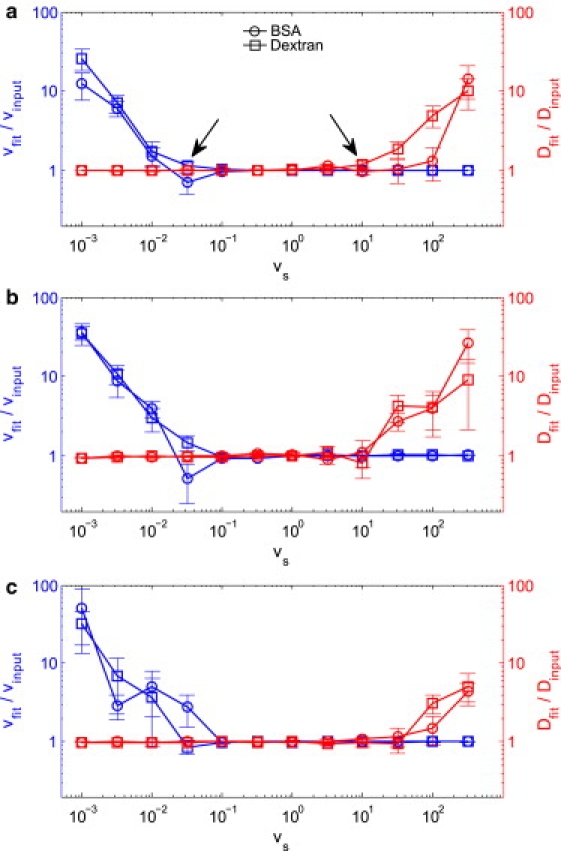
Conditions for accurate fitting using the diffusion-convection model, as assessed by fitting computer-generated data. Fluorescence recovery curves were generated with the diffusion-convection model, keeping the bleach-depth parameter and noise level constant while exploring a range of flow speeds (plotted logarithmically) for each of two diffusion coefficients representing BSA and 2000 kDa dextran. The data were fit to the diffusion-convection model, and the diffusion coefficients (red) and flow speeds (blue) produced by the fits were normalized to associated input values. Hence, an accurate result produces a ratio of one. In the case that either diffusion or flow dominates the recovery, the fit poorly determines the nondominant parameter. For a wide range of balanced recoveries, both diffusion and flow are well determined. (a) β = 0.6 and N/S = 3%, experimentally representative values. Arrows point to regimes where the standard deviations in the nondominant parameter are high, even though the average normalized value is close to one. (b) β = 0.6 and N/S = 5%; the increase in noise narrows the balanced regime. (c) β = 1.0 and N/S = 3%; the deeper bleach depth widens the balanced regime.
By producing fits to computer-generated data, we have gained important knowledge of the scaling behavior of recovery curves influenced by diffusion and convection. Verifying the diffusion-convection model in subsequent in vitro tests could require, in principle, hundreds of combinations of flow speeds and tracer molecules. However, by taking advantage of the scaling behavior depicted in Fig. 3, we can demonstrate the physical accuracy of the diffusion-convection model using just two tracer molecules and a moderate range of flow speeds. We also determined a range of conditions (recovery parameters, noise, focal volume) over which we can expect to recover accurate diffusion coefficients when fitting experimental curves with the diffusion-convection model, as well as developed expectations for the behavior of our data statistics. For example, we predict that the error in recovering the diffusion coefficient using both the diffusion-only and diffusion-convection models will increase with increasing flow speed, while for some range of low flow speeds both models will produce accurate diffusion coefficients. We also predict that there will be a range of flow speeds over which the diffusion-convection model produces accurate diffusion coefficients and flow speeds, and a range of flow speeds over which the diffusion-convection model produces only accurate flow speeds. Further, we predict that, using the diffusion-convection model, the standard deviation of the nondominant parameter will increase before the average ratio of Dfit/Dinput or vfit/vinput begins to deviate from one, while the diffusion-only model, lacking a nondominant parameter, will produce very precise, but very inaccurate, values of D as flow increases.
In vitro MP-FRAP
For a direct measure of the conditions necessary to yield accurate fits to the diffusion coefficient using the two models, as well as for verification of the physical accuracy of the new diffusion-convection model, we designed an experimental system with known diffusion and known directed flow. FITC-BSA and FITC-dextran were used as fluorescent tracer molecules. The dramatic difference in molecular weight, 64 kDa and 2000 kDa for BSA and dextran, respectively, was necessary to access the widest range of relevant scaled speeds as suggested by the results of fitting computer-generated data. To determine accuracy of fit, the fit diffusion coefficient was compared against the diffusion coefficient for a diffusion-only system, i.e., performed without experimental flow and fit to the diffusion-only model, and the fit speed was compared against the speed obtained from line-scan data taken concurrently with the MP-FRAP measurements. In the literature, diffusion-coefficient values for BSA vary from 55 to 62 μm2/s (6,27,40–43), while values for dextran range from 8.4 to 9.1 μm2/s (42,43), when adjusted to 20°C via the Stokes-Einstein relation. Our diffusion-only measurements yielded 52 ± 0.7 μm2/s and 9.2 ± 0.05 μm2/s for BSA and dextran, respectively, consistent with the literature.
The results of our measurements with flow are summarized in Figs. 5 and 6. Fig. 5 compares results of the accuracy of the diffusion coefficient as given by both the diffusion-only (circles) and diffusion-convection (diamonds) models for the same collection of data. As predicted from fits to the computer-generated data, the standard deviation in the results from experimental data fit by the diffusion-only model does not increase, even as the error becomes great (i.e., ). To determine a cutoff speed beyond which the diffusion-only model no longer produces an accurate diffusion coefficient, we define an inaccurate fit by the diffusion-only model as one in which Dfit/Do is statistically greater than 1.2 (determined by a one-sided hypothesis test), and we see that the diffusion-only model begins yielding inaccurate fits to the diffusion coefficient at a cutoff value of vs ≈ 0.3. The diffusion-convection model, meanwhile, continues to provide accurate values for the diffusion coefficient for significantly greater flow speeds.
Figure 5.
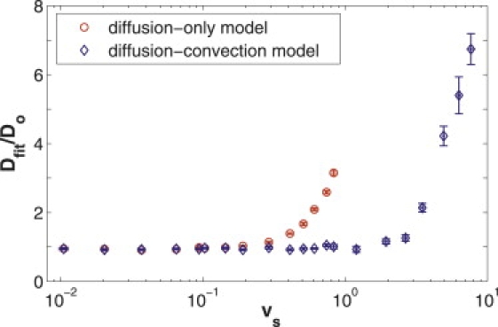
Comparison of in vitro experimental data with flow, fit to the diffusion-only and diffusion-convection models. A series of experimental fluorescence recovery curves for FITC-BSA and FITC-2000 kDa dextran were taken over a wide range of known flow speeds (plotted logarithmically). The curves were then fit to both the diffusion-only (circles) and the diffusion-convection (diamonds) models, and the diffusion coefficients produced by each fit were normalized to the value measured in a system without flow and fit to the diffusion-only model. Hence, an accurate result produces a ratio of one. As the flow speed grows beyond vs ≈ 0.3, the diffusion-only model yields an increasing overestimate to the diffusion coefficient. The improved diffusion-convection model, however, continues to provide accurate diffusion coefficients for scaled speeds up to vs ≈ 3, ∼10 times larger than the cutoff speed for the diffusion-only model.
Figure 6.
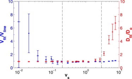
Results of fitting in vitro experimental data with flow to the diffusion-convection model. A series of experimental fluorescence recovery curves for FITC-BSA and FITC-2000 kDa dextran were taken over a wide range of known flow speeds (plotted logarithmically). The diffusion coefficients (red) taken from the respective fits to the diffusion-convection model are presented here as ratios with respect to the associated diffusion coefficient measured in a system without flow and fit to the diffusion-only model. The flow speeds (blue) taken from the fits are presented as ratios with respect to flow speeds measured via line-scans. An accurate result produces a ratio of one. As with the computer-generated data, when either diffusion or flow dominates the fluorescence recovery, the fit correctly determines the dominant parameter, but poorly determines the nondominant parameter. For a wide range of balanced recoveries, 0.2 ≲ vs ≲ 3, both parameters are determined accurately. Dotted lines delineate the two experimentally determined cutoff speeds that define the parameter spaces in which the diffusion-convection model accurately determines one (or both) parameters.
Fig. 6 displays the accuracy of the results for both the diffusion coefficient and the flow speed as determined by fitting data with the diffusion-convection model. For the diffusion-convection model, our fits to computer-generated data indicated that the standard deviation in fit values of the nondominant parameter can increase before deviations from one arise in the ratio of Dfit/Do or vfit/vlinescan. We therefore define a poor measurement as having a standard deviation >15% of the mean value. Using this criterion, we can expect the transition from diffusion-dominated to a balanced recovery to occur at vs ≈ 0.2 and the transition from balanced to a flow-dominated recovery to occur at vs ≈ 3. These experimentally determined cutoff speeds are valid for β ≈ 0.5 and relative noise ≈ 4%, chosen to match typical experimental values (37). While our fits to generated data have shown that differing amounts of noise and bleach-depth will shift these cutoff values slightly (see Fig. 4), we can use these cutoff values as estimates of the range of behaviors expected for in vivo experiments.
We also tested the ability of the diffusion-convection model to measure diffusion in the presence of flow in the axial direction (perpendicular to the imaging plane). With this geometry, it was not feasible to measure flow speeds via line-scans for independent verification. However, by choosing a reservoir height corresponding to a relatively modest flow, we produced a diffusion coefficient for FITC-BSA of 51 ± 2 μm2/s (vs = 0.9 ± 0.2 based on velocity values taken from the fit), which matched our same-day measurement of diffusion in a flow-free system, D = 53 ± 4 μm2/s (p = 0.42, N = 5). In addition, for a relatively high rate of flow, we found D = 59 ± 2 μm2/s (vs = 4 ± 0.5), which was statistically larger than the flow-free measurement (p = 0.0042, N = 5). These results compare well with those derived from measurements taken within the imaging plane.
In vivo MP-FRAP
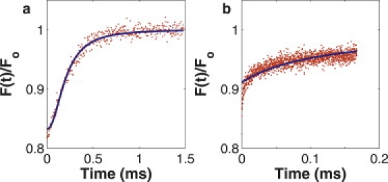
We chose to demonstrate the effectiveness of the diffusion-convection model in vivo by measuring diffusion (and convection) within living tumor vessels. This model was selected because blood flow through tumor vessels exhibits a wide range of flow speeds with which to fully test the diffusion-convection model in vivo in analogy with our in vitro experimentation. Moreover, measurement of plasma viscosity (using a simple conversion via the Stokes-Einstein equation) has important applications in the study of several disease states. By choosing vessels parallel to the plane of imaging, we could continue to employ the line-scan technique to measure the red blood cell (RBC) speed, which was used as an independent in vivo measurement of transverse flow to compare with our MP-FRAP flow speed measurements. Fig. 7 shows representative recovery curves and associated fits to the diffusion-convection model for FITC-dextran flowing in three different tumor vessels. Table 1 shows the results of fitting the curves to both the diffusion-only and diffusion-convection models, as well as the average RBC speed in that part of the vessel. We have also tabulated the value of the predicted flow scaled speed, vs, as calculated from RBC speeds and in vitro diffusion coefficient measurements (adjusted to 37°C and η = 1.2 cP, the viscosity of plasma (44), via the Stokes-Einstein relation). Please note that the data presented for vs and vRBC represent the mean and standard error of five measurements, while the data presented for Ddiff–only, Ddiff–conv, and vdiff–conv represent the fit values from each of three single data curves and the associated error in the fitted parameters. The presence of pulsatile flow caused flow rates to vary within individual vessels, and particularly widely in larger vessels, thus preventing the calculation of meaningful means and standard deviations for speed values. (In this case, the mean and standard deviation would describe the variation in the speed, not the variation in the ability of the diffusion-convection model to fit the data accurately.)
Figure 7.
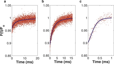
Experimental fluorescence recovery curves of FITC-dextran, flowing in vessels of 4T1 tumors growing in dorsal skinfold chambers. Each curve represents a different fitting regime for the diffusion-convection model. (a) Diffusion-dominated recovery; only the diffusion coefficient is accurately determined. (b) Balanced recovery; both the diffusion coefficient and flow speed are accurately determined. (c) Flow-dominated recovery; only the flow speed is accurately determined.
Table 1.
Results of fitting experimental in vivo data of diffusion and convection in tumor vessels using both the diffusion-only and diffusion-convection models
| vs∗ | Dd† (μm2/s) | Dd–c† (μm2/s) | vd–c† (μm/s) | vRBC∗ (μm/s) | |
|---|---|---|---|---|---|
| Vessel 1 | 0.08 ± 0.02 | 9.3 ± 0.5 | 9.3 ± 0.5 | 0.02 ± 2000 | 14 ± 3 |
| Vessel 2 | 0.45 ± 0.05 | 19.6 ± 0.4 | 9.7 ± 0.3 | 70 ± 1 | 80 ± 10 |
| Vessel 3 | 6.2 ± 0.4 | 250 ± 25 | 35 ± 10 | 990 ± 40 | 1140 ± 80 |
Reported error is ± error of the mean, n = 5.
Reported error is ± standard error in fitted parameter, n = 1.
In vessel 1, we see that the RBC speed was 14 ± 3 μm/s, producing a predicted scaled speed of 0.08 ± 0.02, well below the estimated cutoff speed for accurate fitting with the diffusion-only MP-FRAP model and comfortably within the diffusion-dominated regime for the diffusion-convection model. From this, we would predict that both models would yield an accurate value for the diffusion coefficient, and that the diffusion-convection model would provide an inaccurate value for the flow speed. As predicted, the two models produce identical values for the diffusion coefficient (D = 9.28 μm2/s), which is consistent with the literature when adjusted via the Stokes-Einstein relation using a plasma viscosity of η = 1.2 cP. Meanwhile, as predicted, a significant difference is evident between the measured flow speed (v = 0.02 ± 2000 μm/s) and the RBC speed (v = 14 ± 3 μm/s).
Vessel 2 has a predicted scaled speed of 0.45 ± 0.05, which is above the cutoff speed for the diffusion-only model but within the balanced regime for the diffusion-convection model. This indicates that the diffusion-only model should overestimate the diffusion coefficient, while the diffusion-convection model should yield accurate results for both the diffusion coefficient and the flow speed. As expected, the diffusion-only model produces an erroneously high diffusion coefficient (D = 19.6 ± 0.4 μm2/s) due to the presence of significant flow. In addition, as predicted, the diffusion-convection model produces a diffusion coefficient (D = 9.68 ± 0.34 μm2/s) that compares well with the value obtained from vessel 1 and with the extrapolated literature value. This suggests that this measurement is not impacted by the increased flow speed. Additionally, the diffusion-convection model yields a result for the flow speed that is comparable to the RBC speed. The slight difference between the plasma speed produced by the diffusion-convection model and the RBC speed produced by the line-scans is statistically significant (69.3 ± 1.0 versus 80 ± 10 μm/s, p = 0.036). However, on the edge of the red blood cell-free layer within blood vessels, it is expected that the RBC speed will be slightly larger than the plasma speed (44).
Vessel 3 has a predicted scaled speed of 6.2, well above the cutoff speed for the diffusion-only model and in the flow-dominated regime for the diffusion-convection model. From this, we expect both models to yield inaccurate results for the diffusion coefficient, while the diffusion-convection model should provide an accurate measure of the flow speed. As predicted, the diffusion-only model produces a diffusion coefficient that is erroneously high (D = 250 ± 24 μm2/s), due to the presence of dominant flow. The diffusion-convection model also produces an erroneously high diffusion coefficient (D = 34.9 ± 9.5 μm2/s). This suggests that the flow in this vessel is rapid enough to produce detectable deviations in diffusion coefficient measurements, even for the diffusion-convection model. Finally, the plasma speed determined by the diffusion-convection model is comparable to the RBC speed, although the small difference between the measured flow speed and the RBC speed is statistically significant (987 ± 36 versus 1140 ± 80 μm/s, p = 0.013). This small difference is again anticipated in tumor vessels, and allows us to conclude that the fit speed value is accurate.
Discussion
MP-FRAP is a well-established microscopy technique used to measure the diffusion of macromolecules within biological systems. However, the presence of unanticipated convective flow can produce erroneous diffusion coefficients when recovery curves are fit with the previously derived diffusion-only model. Here we have derived a new diffusion-convection model for fitting MP-FRAP recovery curves, which improves upon the diffusion-only model by enabling accurate determination of the diffusion coefficient in the presence of significant convective flows. We have evaluated this new model by fitting computer-generated recovery curves with convective flow and by conducting in vitro experiments with known flows and known diffusion coefficients as a means of evaluating the physical accuracy of the model and quantifying the advantages of the diffusion-convection model compared with the diffusion-only model. We have also demonstrated the new MP-FRAP model in measurements of the diffusion coefficient and flow speed in vivo within tumor blood vessels.
Diffusion-only MP-FRAP model
As shown in Figs. 3 and 5, the diffusion-only model yields accurate values for the diffusion coefficient at negligible flows in both computer-generated data and in vitro experiments. As flows become appreciable and increase the rate of recovery, the diffusion-only model compensates by erroneously raising the diffusion coefficient in the resulting fit. At extremely high flow speeds, this error is obvious to the experimentalist as the shape of the recovery curve changes dramatically and the diffusion-only model fit becomes visibly poor (Fig. 8 a). However, when flow only moderately influences the recovery, the shape change is subtle and the diffusion-only model may still yield a good looking fit while offering an inaccurate diffusion coefficient (Fig. 8 b). Herein lies the danger when the diffusion-only model is applied to an unfamiliar system with modest convective flow. This effect can be quantified with our experimentally derived cutoff scaled speed of vs ≈ 0.3. For scaled speeds greater than this value, at typical relative noise values, fitting with the diffusion-only model will yield erroneous values of the diffusion coefficient.
Figure 8.
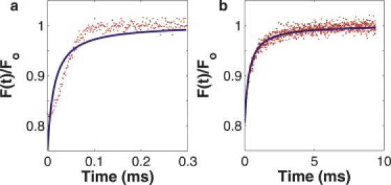
Computer-generated fluorescence recovery curves, generated with the diffusion-convection model and fit to the diffusion-only model. (a) The recovery is flow-dominated and there is an obvious alteration in the shape of the recovery curve, which is visibly poorly fit by the diffusion-only model. (b) The recovery is balanced under the influences of diffusion and flow. Although the fit looks good by eye, the diffusion-only model produces a diffusion coefficient 25% larger than the input value.
Diffusion-convection MP-FRAP model
The diffusion-convection model offers a significant improvement over the diffusion-only model by yielding accurate diffusion coefficients in the presence of flows significant enough to generate errors in the diffusion coefficient when fit by the diffusion-only model. As an added benefit, the diffusion-convection model is also capable of accurately determining the flow speed over some range of parameters. However, fits to computer-generated and in vitro data show that when either diffusion or flow dominates the fluorescence recovery, the diffusion-convection model poorly determines the nondominant parameter, thus setting up three regimes: 1), diffusion-dominated, in which only the diffusion coefficient is accurately determined; 2), balanced, in which both the diffusion coefficient and flow speed are accurately determined; and 3), flow-dominated, in which only the flow speed is accurately determined. By defining a scaled speed parameter, vs = v(ωr/8D), each of the two transitions between the regimes can be seen to occur over the same range of scaled speeds for all magnitudes of diffusion coefficients. These transitions will shift slightly when fluorescence recoveries with differing amounts of relative noise and/or bleach depths are analyzed, such that the balanced regime is broadest with low noise and/or high bleach depth and is narrowest with high noise and/or low bleach depth.
As a direct experimental measure of the abilities of the diffusion-convection model, we conducted MP-FRAP in a simple system with known flow speeds, using a fluorescent dye conjugated to a macromolecule (BSA or dextran) with a known diffusion coefficient. In agreement with the fits to computer-generated data, a comparison of fits of the in vitro data to the diffusion-only and diffusion-convection models showed that the diffusion-convection model yields accurate diffusion coefficients for flow speeds up to ∼10 times the value of the maximum speed at which the diffusion-only model was able to yield an accurate diffusion coefficient. In addition, as expected, when flow speeds were appreciable yet small, the diffusion-convection model accurately determined the diffusion coefficient, but poorly determined the flow speed. Specifically, for typical experimental noise (∼4%) and bleach depth (∼0.5), the cutoff speed for transition from diffusion-dominated to balanced recoveries was vs ≈ 0.2, while the cutoff speed for transition from balanced to flow-dominated recoveries was vs ≈ 3. For both transitions, the standard deviation of the measured value of the nondominant parameter was a more sensitive indicator of problems with the fit than was the average value of the nondominant parameter. We also applied the diffusion-convection model to recovery curves taken in the presence of axial flows (perpendicular to the imaging plane), and showed that the model correctly recovers the diffusion coefficient. By extension, with a priori knowledge of the flow direction, the diffusion-convection model could be used to determine the diffusion coefficient (and flow speed) for multidimensional flows without increasing the number of fitting parameters.
It is also important to note that the choice of tracer molecule significantly affects the ability to accurately measure the diffusion coefficient in the presence of convective flow. Given that the cutoff scaled speed values are constant with relation to the value of the diffusion coefficient, and that vs = v(ωr/8D), we see that the larger the diffusion coefficient is for a given tracer, the smaller the scaled speed will be for any particular absolute speed. To keep the scaled speed below the cutoff between the balanced and flow-dominated regimes (where diffusion can no longer be accurately measured), systems with large flow speeds are best probed with small molecules (typically having a large diffusion coefficient), whereas systems with small flow speeds are as accurately probed with small or large molecules (typically having a large or small value of the diffusion coefficient, respectively).
In vivo application
As an analogous demonstration of the diffusion-convection model in vivo to compare with our in vitro results, we chose to measure diffusion and convection within tumor blood vessels. The RBC speed provided a separate indicator of flow speeds with which to evaluate our model. Our first example was a vessel with an extremely slow RBC speed, and hence a low scaled speed of 0.08 (calculated using our in vitro values of the diffusion coefficient extrapolated to plasma at 37°C). From this scaled speed value, we predicted that accurate values for the diffusion coefficient would be produced by both the diffusion-only and the diffusion-convection models, but that an inaccurate value for the flow speed would be given by the diffusion-convection model, due to the dominance of diffusion over flow. Our second example was a vessel with a scaled speed of 0.45, in between the two transition cutoff speeds, suggesting that the diffusion-only model would be unable to produce an accurate value for the diffusion coefficient, while the diffusion-convection model would accurately determine both the diffusion coefficient and flow speed. Our third example was a vessel with a scaled speed of 6.24, above the highest transition cutoff speed, and predicting inaccurate values for the diffusion coefficient from both models, but an accurate flow speed from the diffusion-convection model. In each case, the in vivo data analyzed as predicted. These examples demonstrate in vivo that the diffusion-convection model extends the range of flow speeds over which accurate diffusion coefficients can be determined by an order of magnitude and that the diffusion-convection model can also determine the flow speed accurately over a wide range of flows.
In addition to the diffusion-convection model described here, an anomalous subdiffusion model has been derived and used as an alternative to the diffusion-only model to fit FRAP and in vivo MP-FRAP curves (37,45,46). An anomalous subdiffusion model can be produced by replacing any Dt terms in the recovery equation (Eq. 3) with Γtα, where Γ is a constant transport coefficient with units μm2/sα and 0 < α < 1 (37). Choosing between models is straightforward, as anomalous subdiffusion and convective flow differentially affect the speed of recovery and the shape of the recovery curve. Graphically, anomalous subdiffusion stretches out MP-FRAP curves, while convective flow adds a kink. By again using computer-generated MP-FRAP curves, we determined that the two models are incompatible. Recovery curves generated using the diffusion-convection model could be fit by the anomalous subdiffusion model with a low χ-squared value, but in the presence of significant convective flow, the added kink causes the anomalous subdiffusion model to produce parameter values grossly out of line with the literature. For example, for a curve generated with vs = 1 (within the balanced regime), the resulting fit to the anomalous subdiffusion model yielded Γ = 1.35 × 106 μm2/sα and α = 2.11 (Fig. 9 a), compared with Γ = 0.7 μm2/sα and α = 0.55 found in the literature (37). Meanwhile, in the presence of significant anomalous subdiffusion, the stretching-out of the curve is visibly very poorly fit by the diffusion-convection model (Fig. 9 b). Of course, in ranges with mildly anomalous subdiffusion (α > 0.85, i.e., close to 1) or small scaled flow speeds (vs < 0.1, i.e., close to 0), low χ-squared fits with reasonable parameter values are produced. In these cases, some a priori knowledge of the system would be necessary to distinguish mildly anomalous subdiffusion from a slow transverse flow speed.
Figure 9.
Mismatch between diffusion-convection and anomalous subdiffusion models. (a) Curve was computer-generated with the diffusion-convection model (D = 52 μm2/s and vs = 1) and fit with the anomalous subdiffusion model. Although the fit looks good, the anomalous parameters are grossly misaligned with the literature (Γ = 1.35 × 106μm2/sα and α = 2.11). (b) Curve was computer-generated with the anomalous subdiffusion model (Γ = 0.7 μm2/sα and α = 0.35) and fit with the diffusion-convection model. The fit is visibly poor (D = 172.08 μm2/s and v = 0.13 μm/s).
Future applications
In future experiments in which both the diffusion coefficient and flow speed are not known a priori, the diffusion-convection model can be used for fitting MP-FRAP curves, and the typical cutoff speeds determined here can act as a retrospective sanity check. If the output diffusion coefficient and flow speed are within the cutoff speeds, one can assume the values are correct. This is because at no point does the absolute error in the nondominant parameter grow large enough to map the incorrect output parameters into the balanced regime. For example, the computer-generated MP-FRAP curves that produced the data on the extreme right-hand side of Fig. 4 were performed at a scaled speed of 300 and produced a normalized diffusion coefficient of 10 and a normalized flow speed of 1. The output scaled speed is hence (incorrectly) determined to be 30. This scaled speed value is erroneously low, but still above the cutoff speed, and hence would be easily rejected by the experimentalist as indicating incorrect values of the fit parameters, even if the fit appears reasonable.
Conclusion
In this article, we derived an improved model of multiphoton fluorescence recovery after photobleaching that explicitly accounts for the presence of convective flow, as well as diffusion. Using computer-generated data to guide our in vitro experiments, we demonstrated that this new model extends the ability of MP-FRAP to determine diffusion coefficients accurately in the presence of flow to flow speeds an order-of-magnitude higher than is possible with the diffusion-only model of MP-FRAP, which does not account for flow. We also determined experimentally useful cutoff speeds that, for typical experimental parameters, predict the range of scaled speeds over which the diffusion-convection model allows MP-FRAP to produce accurate diffusion coefficients, as well as accurate flow speeds.
Appendix
The time-dependent concentration of unbleached fluorophore immediately after the termination of a bleach pulse is given by Brown et al. (37). When converted to Cartesian coordinates, this is given by
| (4) |
where
| (5) |
| (6) |
| (7) |
An attenuated laser beam is used to monitor the changing concentration profile. The fluorescence recovery is given by (37)
| (8) |
where δm is the multiphoton fluorescence action cross section, 〈Immo(x, y, z)〉 is the time-average of the bleach intensity raised to the mth power, and m is the number of photons required to produce fluorescence from a single fluorophore.
We first consider flow along the x axis. To solve for F(t) in this case, we choose a frame of reference in which we have a source moving along the x direction (the concentration distribution moving under flow) and a stationary observer (the focal volume monitoring the intensity). In the frame of reference of the observer, x′ = x + vt, y′ = y, and z′ = z. The time-dependent fluorophore concentration is now
| (9) |
The expression for the monitoring intensity distribution does not change from the case of both source and observer stationary (37):
| (10) |
Substituting Eqs. 9 and 10 into Eq. 8 yields
| (11) |
Before integrating, we first rewrite the exponential in x′ by expanding the exponent, completing the square in x′, then making the variable substitution:
| (12) |
The expression for the fluorescence recovery now looks like
| (13) |
where
| (14) |
The integrals in Eq. 13 are now all first-order Gaussians. When the integrals are performed and , μn(t), and νn(t) have been substituted in, the simplified expression, letting m = b = 2 for a two-photon process, is
| (15) |
We may also express the equation in terms of system-specific variables, τD = ωr2/8D and τv = ωr/v:
| (16) |
This equation can be generalized to flow with a component along all three axes (v2 = vx2 + vy2 + vz2) as
| (17) |
where , , and . Finally, we can express this equation in cylindrical coordinates, to mimic the symmetry of the two-photon focal volume,
| (18) |
where and . Note that vr is not a radial velocity (this would imply a divergence), but rather the resultant velocity obtained by adding the velocity components within the image plane (vx and vy) vectorially. Because the radial and axial dimensions of the two-photon focal volume are not equal, the velocity components parallel and perpendicular to the image plane cannot be combined into a coordinate-free resultant velocity. The decision to use Eq. 16, 17, or 18 depends on the experimentalist's knowledge of the direction of the flow. Use of the one-dimensional form, Eq. 16, is justified in this work because the in vitro experiments were designed to allow flow predominantly in one direction and the flow within blood vessels, measured in vivo, is directed parallel to the vessel wall.
Acknowledgments
Special thanks to Ryan Burke for overseeing all cell and tissue culture, and to Khawarl Liverpool for his careful dorsal skinfold chamber surgeries.
This work was funded by a Department of Defense Era of Hope Scholar Award (No. W81XWH-05-1-0396) and a Pew Scholar in the Biomedical Sciences Award to E.B.B. III.
References
- 1.Peters R., Peters J., Tews K., Bahr W. Microfluorimetric study of translational diffusion of proteins in erythrocyte membranes. Biochim. Biophys. Acta. 1974;367:282–294. doi: 10.1016/0005-2736(74)90085-6. [DOI] [PubMed] [Google Scholar]
- 2.Axelrod D., Koppel D.E., Schlessinger J., Elson E., Webb W.W. Mobility measurement by analysis of fluorescence photobleaching recovery kinetics. Biophys. J. 1976;16:1055–1069. doi: 10.1016/S0006-3495(76)85755-4. [DOI] [PMC free article] [PubMed] [Google Scholar]
- 3.Edidin M., Zagyansky M., Lardner T. Measurement of membrane protein lateral diffusion in single cells. Science. 1976;191:466–468. doi: 10.1126/science.1246629. [DOI] [PubMed] [Google Scholar]
- 4.Schlessinger J., Koppel D.E., Axelrod D., Jacobson K., Webb W.W. Lateral transport on cell membranes: mobility of convalin A receptors on myoblasts. Proc. Natl. Acad. Sci. USA. 1976;73:2409–2413. doi: 10.1073/pnas.73.7.2409. [DOI] [PMC free article] [PubMed] [Google Scholar]
- 5.Tsay T.-T., Jacobson K.A. Spatial Fourier analysis of video photobleaching measurements. Biophys. J. 1991;60:360–368. doi: 10.1016/S0006-3495(91)82061-6. [DOI] [PMC free article] [PubMed] [Google Scholar]
- 6.Berk D.A., Yuan F., Leunig M., Jain R.K. Fluorescence photobleaching with spatial Fourier analysis: measurement of diffusion in light-scattering media. Biophys. J. 1993;65:2428–2436. doi: 10.1016/S0006-3495(93)81326-2. [DOI] [PMC free article] [PubMed] [Google Scholar]
- 7.Denk W., Strickler J.H., Webb W.W. Two-photon laser scanning fluorescence microscopy. Science. 1990;248:73–76. doi: 10.1126/science.2321027. [DOI] [PubMed] [Google Scholar]
- 8.Brown E.B., Campbell R.B., Tsuzuki Y., Xu L., Carmeliet P. In vivo measurement of gene expression, angiogenesis, and physiological function in tumors using multi-photon laser scanning microscopy. Nat. Med. 2001;7:864–868. doi: 10.1038/89997. [DOI] [PubMed] [Google Scholar]
- 9.Brown E.B., Boucher Y., Nasser S., Jain R.K. Measurement of macromolecular diffusion coefficients in human tumors. Miscrovasc. Res. 2004;67:231–236. doi: 10.1016/j.mvr.2004.02.001. [DOI] [PubMed] [Google Scholar]
- 10.Dunn K.W., Sandoval R.M., Kelly K.J., Dagher P.C., Tanner G.A. Functional studies of the kidney of living animals using multicolor two-photon microscopy. Am. J. Physiol. Cell Physiol. 2002;283:C905–C916. doi: 10.1152/ajpcell.00159.2002. [DOI] [PubMed] [Google Scholar]
- 11.Molitoris B.A., Sandoval R.M. Intravital multiphoton microscopy of dynamic renal processes. Am. J. Physiol. Renal Physiol. 2005;288:F1084–F1089. doi: 10.1152/ajprenal.00473.2004. [DOI] [PubMed] [Google Scholar]
- 12.Sipos A., Toma I., Kang J., Rosivall L., Peti-Peterdi J. Advances in renal (patho)physiology using multiphoton microscopy. Kidney Int. 2007;72:1188–1191. doi: 10.1038/sj.ki.5002461. [DOI] [PMC free article] [PubMed] [Google Scholar]
- 13.Rosivall L., Mirzahosseini S., Toma I., Sipos A., Peti-Peterdi J. Fluid flow in the juxtaglomerular interstitium visualized in vivo. Am. J. Physiol. Renal Physiol. 2006;291:1241–1247. doi: 10.1152/ajprenal.00203.2006. [DOI] [PubMed] [Google Scholar]
- 14.Kuricheti K.K., Buschmann V., Weston K.D. Application of fluorescence correlation spectroscopy for velocity imaging in microfluidic devices. Appl. Spectrosc. 2004;58:1180–1186. doi: 10.1366/0003702042335957. [DOI] [PubMed] [Google Scholar]
- 15.Squires T., Quake S. Microfluidics: fluid physics at the nanoliter scale. Rev. Mod. Phys. 2005;77:977–1026. [Google Scholar]
- 16.Kim D.R., Zheng X. Numerical characterization and optimization of the microfluidics for nanowire biosensors. Nano Lett. 2008;8:3233–3237. doi: 10.1021/nl801559m. [DOI] [PubMed] [Google Scholar]
- 17.Késmárky G., Kenyeres P., Rábai M., Tóth K. Plasma viscosity: a forgotten variable. Clin. Hemorheol. Microcirc. 2008;39:243–246. [PubMed] [Google Scholar]
- 18.James D.R. The hyperviscosity syndrome. Br. J. Oral Surg. 1974;12:56–62. doi: 10.1016/0007-117x(74)90061-4. [DOI] [PubMed] [Google Scholar]
- 19.Junker R., Heinrich J., Ulbrich H., Schulte H., Schönfeld R. Relationship between plasma viscosity and the severity of coronary heart disease. Arterioscler. Thromb. Vasc. Biol. 1998;18:870–875. doi: 10.1161/01.atv.18.6.870. [DOI] [PubMed] [Google Scholar]
- 20.Kensey K.R. The mechanistic relationships between hemorheological characteristics and cardiovascular disease. Curr. Med. Res. Opin. 2003;19:587–596. doi: 10.1185/030079903125002289. [DOI] [PubMed] [Google Scholar]
- 21.Lowe G., Fowkes F., Dawes J., Donnan P., Lennie S. Blood viscosity, fibrinogen, and activation of coagulation and leukocytes in peripheral arterial disease and the normal population in the Edinburgh Artery Study. Circulation. 1993;87:1915–1920. doi: 10.1161/01.cir.87.6.1915. [DOI] [PubMed] [Google Scholar]
- 22.Coull B.M., Beamer N., de Garmo P., Sexton G., Nordt F. Chronic blood hyperviscosity in subjects with acute stroke, transient ischemic attack, and risk factors for stroke. Stroke. 1991;22:162–168. doi: 10.1161/01.str.22.2.162. [DOI] [PubMed] [Google Scholar]
- 23.Mehta J., Singhal S. Hyperviscosity syndrome in plasma cell dyscrasias. Semin. Thromb. Hemost. 2003;29:467–471. doi: 10.1055/s-2003-44554. [DOI] [PubMed] [Google Scholar]
- 24.von Tempelhoff G.-F., Heilmann L., Hommel G., Pollow K. Impact of rheological variables in cancer. Semin. Thromb. Hemost. 2003;29:499–513. doi: 10.1055/s-2003-44641. [DOI] [PubMed] [Google Scholar]
- 25.International Committee for Standardization in Hematology Guidelines on selection of laboratory tests for monitoring the acute phase response. J. Clin. Path. 1998;41:1203–1212. doi: 10.1136/jcp.41.11.1203. [DOI] [PMC free article] [PubMed] [Google Scholar]
- 26.Berk D.A., Swartz M.A., Leu A.J., Jain R.K. Transport in lymphatic capillaries. II. Microscopic velocity measurement with fluorescence photobleaching. Am. J. Physiol. 1996;270:H330–H337. doi: 10.1152/ajpheart.1996.270.1.H330. [DOI] [PubMed] [Google Scholar]
- 27.Chary S.R., Jain R.K. Direct measurement of interstitial convection and diffusion of albumin in normal and neoplastic tissues by fluorescence photobleaching. Proc. Natl. Acad. Sci. USA. 1989;86:5385–5389. doi: 10.1073/pnas.86.14.5385. [DOI] [PMC free article] [PubMed] [Google Scholar]
- 28.Jain R.K., Stock R.J., Chary S.R., Rueter M. Convection and diffusion measurements using fluorescence recovery after photobleaching and video calibration. Microvasc. Res. 1990;39:77–93. doi: 10.1016/0026-2862(90)90060-5. [DOI] [PubMed] [Google Scholar]
- 29.Madge D., Webb W.W., Elson E.L. Fluorescence correlation spectroscopy. III. Uniform translation and laminar flow. Biopolymers. 1974;17:361–376. doi: 10.1002/bip.1974.360130103. [DOI] [PubMed] [Google Scholar]
- 30.Qian H., Sheetz M.P., Elson E.L. Single particle tracking. Analysis of diffusion and flow in two-dimensional systems. Biophys. J. 1991;60:910–921. doi: 10.1016/S0006-3495(91)82125-7. [DOI] [PMC free article] [PubMed] [Google Scholar]
- 31.Saxton M.J., Jacobson K. Single-particle tracking: applications to membrane dynamics. Annu. Rev. Biophys. Biomed. 1997;26:373–399. doi: 10.1146/annurev.biophys.26.1.373. [DOI] [PubMed] [Google Scholar]
- 32.Berland K.M., So P.T.C., Gratton E. Two-photon fluorescence correlation spectroscopy: method and application to the intracellular environment. Biophys. J. 1995;68:694–701. doi: 10.1016/S0006-3495(95)80230-4. [DOI] [PMC free article] [PubMed] [Google Scholar]
- 33.Mertz J., Xu C., Webb W.W. Single-molecule detection by two-photon excited fluorescence. Opt. Lett. 1995;20:2532–2534. doi: 10.1364/ol.20.002532. [DOI] [PubMed] [Google Scholar]
- 34.Wiseman P.W., Squier J.A., Ellisman M.H., Wilson K.R. Two photon image correlation spectroscopy and image cross-correlation spectroscopy. J. Microsc. 2000;200:14–25. doi: 10.1046/j.1365-2818.2000.00736.x. [DOI] [PubMed] [Google Scholar]
- 35.Kolin D.L., Ronis D., Wiseman P.W. k-space image correlation spectroscopy: a method for accurate transport measurements independent of fluorophore photophysics. Biophys. J. 2006;91:3061–3075. doi: 10.1529/biophysj.106.082768. [DOI] [PMC free article] [PubMed] [Google Scholar]
- 36.Hebert B., Costantino S., Wiseman P.W. Spatiotemporal image correlation spectroscopy (STICS) theory, verification, and application to protein velocity mapping in living CHO cells. Biophys. J. 2005;88:3601–3614. doi: 10.1529/biophysj.104.054874. [DOI] [PMC free article] [PubMed] [Google Scholar]
- 37.Brown E.B., Wu E.S., Zipfel W., Webb W.W. Measurement of molecular diffusion in solution by multiphoton fluorescence photobleaching recovery. Biophys. J. 1999;77:2837–2849. doi: 10.1016/S0006-3495(99)77115-8. [DOI] [PMC free article] [PubMed] [Google Scholar]
- 38.Kleinfeld D., Mitra P.P., Helmchen F., Denk W. Fluctuations and stimulus-induced changes in blood flow observed in individual capillaries in layers 2 through 6 of rat neocortex. Proc. Natl. Acad. Sci. USA. 1998;95:15741–15746. doi: 10.1073/pnas.95.26.15741. [DOI] [PMC free article] [PubMed] [Google Scholar]
- 39.Leunig M., Yuan F., Menger M.D., Boucher Y., Goetz A.E. Angiogenesis, microvascular architecture, microhemodynamics, and interstitial fluid pressure density during early growth in human adenocarcinoma LS 174T in SCID mice. Cancer Res. 1992;52:6553–6560. [PubMed] [Google Scholar]
- 40.Lanni F., Taylor D.L., Ware B.R. Fluorescence photobleaching recovery in solutions of labeled actin. Biophys. J. 1981;35:351–364. doi: 10.1016/S0006-3495(81)84794-7. [DOI] [PMC free article] [PubMed] [Google Scholar]
- 41.Bor Fuh C., Levin S., Giddings J.C. Rapid diffusion coefficient measurements using analytical SPLITT fractionation: application to proteins. Anal. Biochem. 1993;208:80–87. doi: 10.1006/abio.1993.1011. [DOI] [PubMed] [Google Scholar]
- 42.Pluen A., Netti P.A., Jain R.K., Berk D.A. Diffusion of macromolecules in agarose gels: comparison of linear and globular configurations. Biophys. J. 1999;77:542–552. doi: 10.1016/S0006-3495(99)76911-0. [DOI] [PMC free article] [PubMed] [Google Scholar]
- 43.Pluen A., Boucher Y., Ramanujan S., McKee T.D., Gohongi T. Role of tumor-host interactions in interstitial diffusion of macromolecules: cranial vs. subcutaneous tumors. Proc. Natl. Acad. Sci. USA. 2001;98:4628–4633. doi: 10.1073/pnas.081626898. [DOI] [PMC free article] [PubMed] [Google Scholar]
- 44.Jain R.K. Determinants of tumor blood flow: a review. Cancer Res. 1988;48:2641–2658. [PubMed] [Google Scholar]
- 45.Feder T.J., Brust-Mascher I., Slattery J.P., Baird B., Webb W.W. Constrained diffusion or immobile fraction on cell surfaces: a new interpretation. Biophys. J. 1996;70:2767–2773. doi: 10.1016/S0006-3495(96)79846-6. [DOI] [PMC free article] [PubMed] [Google Scholar]
- 46.Perisamy N., Verkman A.S. Analysis of fluorophore diffusion by continuous distributions of diffusion coefficients: applications of photobleaching measurements of multicomponent and anomalous diffusion. Biophys. J. 1998;75:557–567. doi: 10.1016/S0006-3495(98)77545-9. [DOI] [PMC free article] [PubMed] [Google Scholar]