Predictions of Phase-Locking in Excitatory Hybrid Networks: Excitation Does Not Promote Phase-Locking in Pattern-Generating Networks as Reliably as Inhibition

Abstract

Phase-locked activity is thought to underlie many high-level functions of the nervous system, the simplest of which are produced by central pattern generators (CPGs). It is not known whether we can define a theoretical framework that is sufficiently general to predict phase-locking in actual biological CPGs, nor is it known why the CPGs that have been characterized are dominated by inhibition. Previously, we applied a method based on phase response curves measured using inputs of biologically realistic amplitude and duration to predict the existence and stability of 1:1 phase-locked modes in hybrid networks of one biological and one model bursting neuron reciprocally connected with artificial inhibitory synapses. Here we extend this analysis to excitatory coupling. Using the pyloric dilator neuron from the stomatogastric ganglion of the American lobster as our biological cell, we experimentally prepared 86 networks using five biological neurons, four model neurons, and heterogeneous synapse strengths between 1 and 10,000 nS. In 77% of networks, our method was robust to biological noise and accurately predicted the phasic relationships. In 3%, our method was inaccurate. The remaining 20% were not amenable to analysis because our theoretical assumptions were violated. The high failure rate for excitation compared with inhibition was due to differential effects of noise and feedback on excitatory versus inhibitory coupling and suggests that CPGs dominated by excitatory synapses would require precise tuning to function, which may explain why CPGs rely primarily on inhibitory synapses.

INTRODUCTION

Synchrony, or phase-locked activity, is thought to underlie complex biological phenomena such as memory, facial recognition, circadian rhythms, and epileptic seizures (de la Iglesia et al. 2004; Fell et al. 2001; Rodriguez et al. 1999). These phenomena are thought to be emergent in the sense that they arise from self-organization of the component elements and cannot be predicted from the individual components without considering their interactions (Strogatz 2003). The most accessible preparations in which to study these phenomena are central pattern generating networks (CPGs). A CPG is a neural network that generates rhythmic output in the absence of rhythmic input. Here we address two outstanding problems in the field: to develop a framework for understanding how patterns emerge from CPGs and to gain insight into the preponderance of inhibitory synapses in such networks.

To gain insight into CPGs, we chose to start with the simplest possible hybrid network comprised of one bursting neuron and one model neuron. Hybrid network construction has the advantage of providing a controlled environment for testing our methodology that incorporates an actual biological neuron and realistic synapses. Endogenously bursting neurons have been shown to be important in the pyloric network (Hartline 1979; Hartline and Gassie 1979; Miller and Selverston 1982), the heartbeat of crustaceans (Tazaki and Cooke 1990), the gastric CPGs of the crustacean stomatogastric system (Harris-Warrick et al. 1992; Panchin et al. 1993; Selverston and Moulins 1987), the feeding CPG in mollusks (Arshavsky et al. 1989, 1991), and appetitive conditioning in the buccal ganglia of Aplysia (Nargeot et al. 1997, 2007). Therefore we chose to examine circuits constructed with endogenous bursters. For the biological neuron, we chose the pacemaking kernel of the pyloric network of the stomatogastric ganglion (STG) in Homarus americanus (Fig. 1 A), comprised of three neurons: the anterior burster (AB) neuron and two pyloric dilator (PD) neurons. The AB/PD complex is electrically coupled and we consider it to be a single functional unit, which we refer to throughout as the biological neuron. The biological neuron was isolated pharmacologically and coupled to a bursting model neuron via excitatory synapses using the dynamic clamp (Fig. 1B).

FIG. 1.

Experimental setup. A: simplified pyloric network. The pacemaking kernel (anterior burster/pyloric dilator [AB/PD] complex) consists of the AB and PD neurons, which are coupled via gap junctions. B: schematic of the dynamic clamp. The membrane voltage recorded in the AB/PD complex was used to calculate synaptic current (I_syn) received by the model cell. The model cell was updated in real time and the updated model neuron's membrane voltage was used to calculate I_syn received by the AB/PD complex. C: measurement of phase resetting in a biological neuron. Shown is a membrane potential recording from a free-running AB/PD complex with intrinsic period P₀, perturbed at ts (dotted vertical line) by an excitatory synaptic input, g_syn = 60 nS and duration = 650 ms. An upward crossing of the voltage threshold (horizontal dashed line; see Phase response curves) was defined as the start of a burst and assigned a phase of zero. The first burst after the perturbation was advanced such that the first perturbed period P₁ was <P₀. The subsequent period P₂ was delayed by a small amount such that P₂ > P₀. In this case, a new burst was triggered after a short delay of 100 ms, so that P₁ > ts and tr = 100 ms. D: measurement of phase resetting in a model neuron. Analogous to the biological neuron, the free-running model neuron was perturbed at ts by an excitatory synaptic input with g_syn = 60 nS. This perturbation was strong and triggered a new burst immediately, such that P₁ ≈ ts and tr ≈ 0. The burst threshold is shown as a horizontal dashed line. (B adapted from DailyClipArt.net.)

A phase response curve (PRC) tabulates the effect of a perturbation on cycle length as a function of the phase at which it is delivered. Our methods use the PRCs of individual component neurons measured in the open-loop configuration with unidirectional synaptic stimuli (Fig. 1, C and D) to predict patterned activity in the closed-loop network configuration with bidirectional coupling. Several assumptions are required so that these PRCs can be used to predict the activity of a network. First, we assume that all component neurons in our circuits exhibit an oscillation in the membrane potential that drives bursting. Quiescent or tonically spiking neurons in the circuit are not within the scope of our methods. Second, we assume that the input received in the closed network is similar to that used to generate the PRC. We do not require the weak coupling assumption that is often used in network analysis (Ermentrout and Chow 2002; Mancilla et al. 2007; Netoff et al. 2005b) and that assumes the phase response is linear. Instead, we make a third assumption—that the effects of one input die out before the next one is received. This is the pulsatile coupling assumption, which treats the perturbation as a whole, reducing the analysis to a cycle-by-cycle mapping, and is equally valid for weak or strong coupling. We consider only 1:1 phase-locking between two bursting neurons in which a stable pattern of activity is established in which each neuron fires one burst per cycle.

To date these methods have been evaluated both in model networks (Achuthan and Canavier 2009; Canavier et al. 1997, 1999; Canavier et al. 2009; Luo et al. 2004; Maran et al. 2008; Oh and Matveev 2008) and in hybrid networks coupled with inhibition (Oprisan et al. 2004). Here we test the applicability of PRC-based firing time maps (Ermentrout and Chow 2002) to excitatory coupling of significant strength and duration, using a wide range of synaptic strengths (from 1 to 10,000 nS) and input durations (from 0.3 to 1.5 s).

Our motivation for studying excitatory synapses was in part to understand why they are less commonly observed in CPGs because all known real CPGs are dominated by inhibitory synapses. Leech heartbeat (Calabrese and Peterson 1983), pyloric and gastric networks of the STG (Marder and Calabrese 1996), lamprey swimming (Cangiano and Grillner 2005), salamander locomotor (Cheng et al. 1998), and mammalian locomotor (McCrea and Rybak 2008) CPGs are all functionally dominated by inhibitory synapses, as evidenced by the lack of a single identified excitatory synapse in the first two systems listed. We present experimental and theoretical data showing that a CPG dominated by typical excitatory synapses would need to be carefully tuned to function and in many configurations would be highly sensitive to noise.

METHODS

Electrophysiology

Homarus americanus were purchased from Inland Seafood (Atlanta, GA). They were maintained in artificial seawater at 10–14°C until used. The stomatogastric nervous system was dissected and pinned out in a dish coated with Sylgard (Dow Corning, Midland, MI) and the STG was desheathed with fine forceps. Throughout the experiments, the stomatogastric nervous system was superfused with chilled (9–14°C) saline containing (in mM) NaCl, 479; KCl, 12; CaCl₂, 18; MgSO₄, 20; Na₂SO₄, 4; and HEPES, 5 (pH 7.45). Extracellular recordings were made with stainless steel pin electrodes in Vaseline wells on the motor nerves and amplified with a differential AC amplifier (Model 1700, A-M Systems, Carlsborg, WA). Intracellular recordings from cells in the STG were obtained with an Axoclamp-2B amplifier (Axon Instruments, Foster City, CA) in discontinuous current-clamp (DCC) mode using microelectrodes filled with 0.6 M K₂SO₄ and 20 mM KCl; electrode resistances were in the range of 10–25 MΩ. Extracellular and intracellular voltage traces were digitized with a Digidata 1200A board (Axon Instruments), recorded using Clampex 9.2 software (Axon Instruments) and analyzed with Spike2 (Cambridge Electronic Design), Matlab (The MathWorks), and in-house software. The AB and PD neurons were identified based on their membrane potential waveforms; the timing of their activity in the pyloric rhythm; and, for PD only, their axonal projections to the appropriate motor nerves. The only chemical synaptic feedback to the pyloric pacemaker group through the lateral pyloric neuron (LP) to PD inhibitory synapse was removed by applying 0.01 mM picrotoxin to the bath. The pharmacologically isolated pyloric pacemaker was monitored by impaling either the AB neuron or one of the PD neurons (Fig. 1A). Experimental preparations were discarded when the pacemaking kernel did not burst consistently.

Dynamic clamp

We recorded the membrane potential of the AB/PD complex and used the dynamic clamp (Prinz et al. 2004; Sharp et al. 1993a,b) to measure biological PRCs and to construct hybrid networks consisting of the AB/PD complex and a model neuron coupled by artificial synapses (Fig. 1B). The membrane potential at the AB or PD cell body was amplified, fed into a National Instruments DAQ board (PCI-6051E), and digitized at 20 kHz. Dynamic-clamp programs were written in C++ and designed to use the Real Time Linux Dynamic Controller (Dorval et al. 2001). One program was written to measure the biological PRC. This program used a membrane potential threshold to detect bursts in the ongoing AB or PD rhythm and monitored the cycle period. Artificial synaptic stimuli were injected at different phases of the rhythm by playing a saved synaptic activation waveform into the artificial synapse (see Phase response curves). This stimulus was a conductance waveform used to calculate the momentary current that would flow through the cell membrane at a given time if the stimulus conductance were present in the membrane. To inject this momentary synaptic current into the AB or PD neuron, the program computed the corresponding command voltage, which was turned into an analog voltage by the DAQ board and sent to the electrode amplifier to compute the synaptic current (described in the next section).

A second program was written to construct hybrid networks. This program implemented two artificial synapses to couple the neurons reciprocally (see Artificial synapses, Fig. 1B). At increments of 50 μs of real time, the following steps were looped: 1) the biological membrane voltage was read from the electrode and used to calculate the synaptic current applied to the model neuron. 2) This current was applied to the model neuron as it was advanced through 50 μs of simulation time. 3) The model membrane voltage was read and used to calculate the synaptic current applied to the biological neuron. 4) This current was applied to the biological neuron. Note that synaptic current was applied “continuously” to the biological neuron using the DCC mode of the Axoclamp amplifier. In step 4, this “continuously” injected current is updated to reflect changes in the presynaptic model neuron. When the model neuron was quiescent, the current delivered to the biological neuron was calculated to be zero. The time resolution of coupling was 50 μs, which was effective to approximate real-time coupling for this system because biological variability of the intrinsic period was relatively large and artificial synapses were sufficiently slow (see Fig. 2 for examples of rise time and fall time of synaptic activation). Biological variability of the intrinsic period was about 10% or 100 ms for a typical burst period.

FIG. 2.

A and B: snippets of free-running membrane voltage traces (black) and synaptic activation variables (gray) are shown for model neurons 1 to 4 (A, top to bottom) and for biological neurons 1 to 5 (B, top to bottom). Dashed lines show burst thresholds specific to each neuron. Timescale for both panels is shown in B. Synaptic activation variable s is unitless.

Artificial synapses

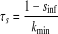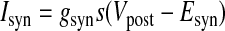
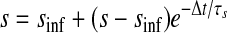
We created hybrid networks by coupling one biological neuron to one model neuron via artificial synapses. Artificial synapses mapped the membrane voltage in one neuron to a synaptic conductance in its partner neuron, so bursts in the presynaptic neuron caused current to be injected in the postsynaptic neuron (Fig. 1B). For all artificial synapses implemented here, the synaptic current I_syn was calculated according to a model of chemical synaptic transmission (Abbott and Marder 1999), where g_syn is the maximal conductance of the synapse, s is the synaptic activation, V_post is the membrane potential of the postsynaptic neuron, s_inf is the asymptotic value of s in time, Δt is the simulation time step, τ_s is the synaptic time constant, V_th is the half-activation voltage of synaptic activation, V_pre is the presynaptic membrane potential, k_min is the backward rate constant of direct ligand binding to the ion channel, and E_syn is the synaptic reversal potential, which was set to 0 mV for all synapses to make them excitatory. V_th and k_min were chosen so that the synapse was fully activated during a presynaptic burst and fully deactivated otherwise. For the networks presented here, Δt = 50 μs, k_min = 0.1 ms⁻¹, and V_th was set equal to the burst threshold of the presynaptic neuron (Fig. 2). Hyperpolarizations between spikes within a burst cause the model neuron voltage to drop below V_th during a burst. The synaptic time constant τ_s (which is controlled by the parameter k_min) acts as a low-pass filter, smoothing repeated crossings of V_th by the model neuron so that bursts are clear in the s trace. For each neuron, this threshold was chosen so that it was in the steepest part of the slow membrane voltage oscillation, giving the highest tolerance to baseline drift. The synaptic activation variable s varies between 0 and 1, so that the synaptic current I_syn is equal to the driving force (V_post − E_syn) scaled by a value between 0 and g_syn. Thus when s = 0, the synapse is “off” (I_syn = 0), whereas when s = 1, the synapse is “on” and I_syn = g_syn(V_post − E_syn). Experimental values of g_syn varied from 1 to 10,000 nS for the biological to model synapse and from 1 to 150 nS for the model to biological synapse. Model to biological synapse strength was limited by stability of the dynamic clamp (Preyer and Butera 2007).

Model neurons

In each hybrid network experiment we used one of four endogenously bursting model neurons, each a single compartment with eight Hodgkin–Huxley-type membrane currents and an intracellular calcium buffer. The membrane currents were based on voltage-clamp experiments on lobster stomatogastric neurons (Turrigiano et al. 1995) and included a fast sodium current (I_NaF), a fast and a slow transient calcium current (I_CaT and I_CaS), a fast transient potassium current (I_A), a calcium-dependent potassium current (I_KCa), a delayed rectifier potassium current (I_Kd), an H-type current (I_H), and a leak current (I_leak). The model neurons differed only in the maximal conductances of their eight membrane currents; these conductances were chosen to produce different burst periods and duty cycles in the different model neurons (Fig. 2A). The model was described in detail in Prinz et al. (2003). Model parameters are given in Table 1. The model was implemented in C++ and all differential equations were integrated with the exponential Euler method (Abbott and Marder 1999) at a time resolution of 50 μs.

TABLE 1.

Model neurons used in this study

Model Neuron	Maximal Conductance, μS
	gNa	gCaT	gCaS	gA	gKCa	gKd	gH	gleak
1	251.32	0.0	6.28	12.57	6.28	15.71	0.03	0.01
2	125.66	0.0	6.28	6.28	12.57	62.83	0.01	0.0
3	251.32	1.57	3.77	25.13	6.28	47.12	0.03	0.0
4	188.49	3.14	6.28	0.0	6.28	47.12	0.03	0.02

The form of these models is given in Prinz et al. (2003) and the maximal conductances for the eight membrane currents are given here.

Phase response curves

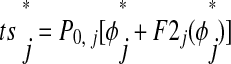
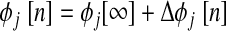
To make phase-locking predictions for each of the 86 hybrid networks we present, we generated 172 PRCs, one for each neuron of each network. The PRC for each component neuron was constructed in open-loop configuration (Fig. 1, C and D) using a pulse in postsynaptic conductance that was elicited by a single spontaneous burst in the partner neuron and parameterized by synaptic strength. Other parameters of the artificial synapse were held constant. For example, to measure the PRCs of biological neuron 1 due to stimulus from model neuron 2 with synapse strength of 30 nS, we first estimated what the profile of synaptic conductance received by the biological neuron would be in a closed-loop network. To do this, we ran a simulation of the model neuron combined with the artificial synapse but isolated from the biological neuron. From this simulation we saved a snippet of the synaptic activation variable s. This snippet was equal to the length of one burst cycle of the model neuron, beginning at the start of a burst, where the synaptic activation variable s rapidly changed from 0 to 1, and ending with the quiescent interval of the neuron, where s was zero (Fig. 2A). To deliver a stimulus, this snippet of s was played into the artificial synapse, which defined the current injected into the biological neuron. The injected conductance was this snippet of s scaled by the maximal conductance of the synapse g_syn. Next, we determined the intrinsic period of the biological neuron, P_0,bio, from 20 consecutive periods of unperturbed activity. We defined P_0,bio as the time between two successive crossings of a voltage threshold with positive slope. This burst threshold was equal to the synaptic parameter V_th so that the synaptic activation and burst thresholds were crossed simultaneously. The slow oscillation was isolated by filtering the voltage waveform according to V_filt(t + Δt) = V_filt(t) + [V(t + Δt) − V_filt(t)]/τ_filt, where V_filt is the filtered waveform, Δt is the time step, and τ_filt = 1 ms. For parity, the filtered voltage V_filt was used for all burst detection in both model and biological neurons. P_0,bio was divided into 100 equally spaced stimulus intervals ts and 100 phase response trials were run. For each value of stimulus phase φ = ts/P₀, ts is the delay from start of burst to start of stimulus, a stimulus is delivered, and the phase response is measured. We define the first-order phase response F1(φ) = (P₁ − P₀)/P₀ and the second-order phase response F2(φ) = (P₂ − P₀)/P₀, where P₁ is the length of the cycle containing the stimulus and P₂ is the length of the subsequent cycle. In each trial, the stimulus was delivered at one value of ts and the first and second perturbed periods P_1,bio and P_2,bio were measured. The recovery interval tr is the interval between stimulus onset and the next burst onset. Figure 3 gives examples of stimuli delivered during the burst (Fig. 3A1 and square in subsequent panels) or immediately after the burst has ended (Fig. 3A2 and triangle in subsequent panels). The bottom traces show the perturbation in conductance (snippet as in Fig. 2A) driven by the model neuron. Burst onset as determined by burst threshold crossing was defined as phase zero φ = 0. Effects on the cycle containing the start of the perturbation were tabulated as first-order resetting F1 (Fig. 3B1) and effects on the next cycle were tabulated as second-order resetting F2 (Fig. 3B2). First- and second-order phase responses F1 and F2 were defined as the amount by which the respective cycle lengths P_1,bio and P_2,bio were extended relative to P_0,bio and they were normalized by P_0,bio (equations in preceding text). By this definition, a positive phase response value indicated a delay of the subsequent burst, whereas a negative value indicated an advance. To ensure that the biological neuron had returned to its unperturbed dynamical activity between stimuli, individual stimuli were delivered four cycles apart. To control for slow adaptation, stimuli were delivered in random order of stimulus phase. Figure 3D shows how F1 and F2 are used to calculate equilibrium intervals ts and tr, denoted throughout this study as ts* and tr*. These are intervals that can be observed in the presence of the repetitive stimulation that occurs in a closed-loop network. As seen in the equations in Fig. 3D, the difference between ts in the open loop and ts* in the closed loop is the F2 term (see next section).

FIG. 3.

Example of phase response curve (PRC) generation and equivalence of information in PRCs vs. ts*–tr* plot. A: membrane voltage traces (top) and injected current (bottom) showing the qualitative difference in response for a stimulus delivered during a burst (A1) vs. one delivered in the quiescent interval between bursts (A2). Dashed horizontal lines in A and B indicate burst thresholds. B: 1st- and 2nd-order PRCs. Black dots denote phase responses measured from individual stimuli. Solid lines are piecewise polynomial fits. For 1st- and 2nd-order PRCs, the order of polynomial fits ranged from 1 to 7 and 1 to 3, respectively. The locations of discontinuities were determined by inspection. Square and triangle marks the data point measured in A1 and A2, respectively. C: schematic showing network connectivity used to measure these PRCs. D: ts*–tr* curve calculated from F1 and F2 in B according to the given equations. This curve represents possible modes of 1:1 phase-locked activity for the biological neuron. The ts*–tr* curve is a parametric function of φ, as described in Theoretical method. Square and triangle marks the phase-locked mode calculated from the data marked in B1 and B2.

PRCs for the model neurons were generated post hoc in an analogous manner. A snippet of the free-running biological voltage trace was used to calculate a snippet of the synaptic activation variable s, which was saved and played into the artificial synapse to stimulate the model neuron. Again, to generate the PRCs F1 and F2, this stimulus was applied at 100 equally spaced intervals of the intrinsic period of the model neuron P_0,mdl.

Mean PRCs used in our analysis were estimated by piecewise polynomial fits to PRC data. The number of polynomial pieces used per PRC ranged from one to three and the order of these polynomials ranged from one to seven. The order of polynomial was chosen to be minimal while maintaining goodness of fit and correct end behavior. To estimate biological variability in the PRCs, envelopes marking the boundary of ±2SDs (σ) were constructed around each mean PRC. This was done by binning each PRC (n = 5) and measuring σ at the center of each bin. Upper and lower envelopes were constructed using piecewise polynomial fits to the mean PRC ±2σ. The number of polynomial pieces used to fit the envelopes was equal to that used for the mean PRC and the order of polynomials used for the envelopes ranged from one to three. The orders of polynomials used to fit envelopes were smaller than those used to fit mean PRCs because the binned data contained fewer data points.

Theoretical method

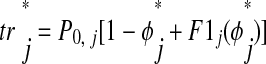
We used the theoretical methods of Oprisan et al. (2004) to predict 1:1 phase-locking in hybrid networks from the PRCs of component neurons. This method first checks for the existence of 1:1 phase-locking using a periodicity criterion then checks that solutions are locally stable by analyzing a linearized version the system. Figure 4 shows the pulse-coupled approximation on which the theoretical method is based (periodicity criterion shown in Fig. 4A). Conduction delays are ignored here, although they can be included in the approximation as shown previously (Oprisan et al. 2004; Woodman and Canavier 2008). Equilibrium stimulus phase φ* and stimulus (recovery) interval ts* (tr*) are defined as φ and ts (tr) earlier, but in the context of an ongoing 1:1 phase-locked mode rather than a single input. Considering only first-order resetting F1_j of neuron j, ts and tr can be calculated as follows

In this case, where second-order resetting is assumed to be zero, ts is the time elapsed between the start of the burst and the onset of input and tr is the fraction of the cycle remaining before the next burst, calculated as 1 − φ plus first-order resetting. The quantities φ and F1_j are unitless. We assume that each neuron returns to its unperturbed limit cycle before it receives a new input (see introduction, third assumption). This is valid because the effects of each input are concluded during the perturbed cycle, before the next input is received, and there is no effect on the subsequent cycle (F2_j is assumed to be zero). In Fig. 4B, neuron 1 receives input during P₁[n] after interval ts₁[n]. The first-order effects of that input are incorporated during the interval tr₁[n] and neuron 1 is allowed to return to its limit cycle by the end of tr₁[n]. The effects of the input received during P₁[n] are concluded by the time neuron 1 receives the next input at the end of the interval ts₁[n + 1]. When considering both F1_j and F2_j, the calculation of tr is the same; however, F2_j affects the subsequent cycle, so ts must be adjusted as follows

In this case, ts is adjusted to include second-order resetting due to input in the previous cycle. Our third assumption is still valid because the next input is not received until ts is complete. The second-order response of an input to a neuron causes the next cycle length to be lengthened or shortened. This effect is presumed to be localized to the ts interval so that when that neuron receives its next input, it has returned to its limit cycle. Thus the effect of F1 is localized to the tr interval of the current cycle and the effect of F2 is localized to the ts interval of the next cycle.

FIG. 4.

Pulse-coupled approximation of a reciprocally coupled bursting network. Gray rectangles represent bursts. Equilibrium intervals ts* and tr* are defined in the text. Conduction delays are ignored. A: definition of intervals during phase-locking between 2 neurons in closed-loop configuration. For phase locking to occur, ts* in the biological neuron (top) must be equal to tr* in the model neuron (bottom) and vice versa. B: convergence to 1:1 phase-locked mode. For a network to satisfy the stability criterion, this cycle-to-cycle mapping of ts[n] and tr[n] must converge to ts₁[∞] = tr₂[∞] and tr₁[∞] = ts₂[∞]. This framework was used to derive a discrete map for the time evolution of the system on a cycle-to-cycle basis. (Figure adapted from Oprisan et al. 2004.)

We can solve for the existence of a 1:1 phase-locked mode using a periodicity criterion, which states that in a 1:1 locking the stimulus interval in one neuron is exactly equal to the recovery interval in the other: ts = tr and tr = ts (Fig. 4A). For a neuron j, any ordered pair (ts, tr) is uniquely determined by the phase φ when that neuron receives input, so these intervals can be considered functions of each other; i.e., functions f and g, ts = f(tr) and tr = g(tr), are both valid because ts and tr are themselves parametric functions of φ (Fig. 3D, equations). Thus satisfaction of the periodicity constraint can be evaluated graphically by plotting ts versus tr and tr versus ts (see Example prediction of a 1:1 phase-locked mode in a hybrid network). Considering the choice of axes, it follows that any intersection of the two curves gives ts = tr and tr = ts. In other words, a phase-locked mode exists at any intersection.

Existence of a mode does not guarantee that it will be observed; it must also be stable, that is, robust to small perturbations. An intersection on a network's ts*–tr* plot uniquely defines a stimulus phase for each neuron, φ and φ (as seen earlier). If the phase-locking defined by this point is also stable, then as cycle number n → ∞, φ_j[n] → φ. To test for stability, PRCs for each neuron are linearized around φ_j[∞] = φ and a return map is constructed that defines the evolution of a small perturbation (Δφ) on a cycle-to-cycle basis. This map (Oprisan and Canavier 2001) is shown in the following text, where n is the cycle number and m_i,j is the linearized slope of the ith order PRC for neuron j at phase φ_j[∞]. Following this definition, m_2,j is the slope of F2(φ_j[∞])

(1)

When F2(φ_j[∞]) ≠ 0, two preceding cycles must be taken into account (n − 1 and n − 2), as shown earlier. Eigenvalues for this two-dimensional map are calculated as follows

When both eigenvalues λ₁ and λ₂ are between −1 and 1, the system is stable.

Inclusion of noise in iterated firing time maps based on the PRC

We modeled a subset of our hybrid networks using the experimentally obtained PRCs of component neurons as well as their noise envelopes. For each component neuron j, interburst intervals (IBIs) were calculated iteratively according to a modified Winfree model (Canavier et al. 1999)

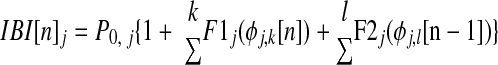where P₀ is the intrinsic period, φ_j,k[n] is the phase at which neuron j receives the kth input in the current cycle, φ_j,l[n − 1] is the phase at which the lth input was received by neuron j in the previous cycle, and F1 and F2 are polynomial fits of experimental PRCs modulated by Gaussian noise matching the distribution of experimental variability described by the envelopes of the appropriate PRCs. This map represents an ideal pulse-coupled system. It differs from the map given in Eq. 1 in that it does not assume a particular firing order. To construct each PRC, a Gaussian noise generator had output scaled to match the magnitude of the noise envelope and this noise was added to the PRC to within causal limits. Each iteration, a new amount of noise was added to the mean fit of the PRC, simulating the experimentally observed variability. To simulate a reduction in the overall amount of noise in the system, we scaled the noise envelope by a factor <1. The inclusion of noise in the PRC-based iterative map is similar to that of Netoff et al. (2005a); the major difference is the use of F2 in addition to F1 in our method.

Hybrid networks

We constructed 86 hybrid networks, each comprised of one biological and one model neuron coupled by artificial excitatory synapses via dynamic clamp (Fig. 1B). Each biological neuron was obtained from a different animal. Synapse strengths ranged from 1 to 10,000 nS, a range that includes conditions of weak and strong couplings, as can be verified by whether the PRCs scale linearly with respect to conductance (weak) or not (strong). For each network, we verified the stable behavior of the biological neuron, then turned on the artificial synapses and recorded the membrane voltages of the biological and model neurons for ≥2 min. Most networks reached steady state within a few seconds. Only steady-state data are reported here. These closed-loop recordings were used to extract experimental values of phase-locked network period and network phase. Synaptic coupling forced some networks into a tonic firing regime. In these cases, we cut short the recording to avoid injecting a large amount of charge into the neuron.

Circular statistics

Circular statistics (Drew and Doucet 1991; Mancilla et al. 2007) were used to summarize observed hybrid network activity. This method allows the presentation of mean and variability of network phase as a single vector. The angle of the vector represents mean network phase [Φ_net on the interval (0, 1)] and is given by

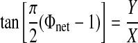where

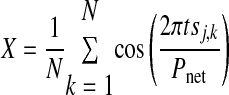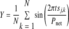where N is the number of bursts recorded in the experiment for neuron j, ts_j,k is the stimulus interval for the kth cycle of neuron j, and P_net is the average network period. The strength of phase-locking is represented by the length of the vector R, where R² = X² + Y². The threshold criterion R² > 0.7 was sufficient to separate networks in which phase-locking was visually obvious from those in which it was not. Instantaneous network phase is represented by the ordered pairs (X_k, Y_k), so that in all circular plots shown, the angle Φ_net = 0 is rightward, Φ_net = ¼ is upward, Φ_net = ½ is leftward, and Φ_net = ¾ is downward.

RESULTS

Example prediction of a 1:1 phase-locked mode in a hybrid network

A typical successful prediction of phase-locking is shown in Fig. 5. Data points from the first- and second-order PRCs for the biological neuron (red dots) were fitted with polynomials (Fig. 5A) and those for the model neuron (blue lines) were generated numerically. These PRCs were used to calculate the ts*–tr* curve for each component neuron (Fig. 5B). The existence of any 1:1 phase-locked modes was determined graphically as the intersections of these curves (Fig. 5B). Noise in the biological neuron was caused primarily by variability in the intrinsic period. The effects of this noise were incorporated in our prediction method by creating an envelope (dashed lines) around the biological PRC and mapping it to the ts*–tr* plot, as was done for the mean PRCs. In this example, there are two intersections on the ts*–tr* plot (blue indicates model tr* as a function of ts*; red indicates biological ts* as a function of tr*), indicating the existence of two modes of phase-locking (Fig. 5B). Our calculations predicted that phase-locking would be stable at only one intersection (arrow). This predicted stable mode of phase-locking was mapped back to phase in the component neurons and indicated using appropriately colored arrowheads (Fig. 5A, arrows).

FIG. 5.

Example of a good prediction. A: PRCs obtained in open-loop configuration from the model (blue) and biological (red) neurons. Raw data points from the biological neuron's PRC are shown, along with a polynomial fit and top and bottom envelopes at ±2σ (dashed lines). Colored arrows indicate stimulus phases for each neuron where the stable mode of synchrony is predicted (see arrow in B). B: graphical method for determining existence of a 1:1 phase-locked mode (ts*–tr* plot). Parametric curves of ts* vs. tr* for model (blue) and biological (red) neurons are shown. Dashed lines indicate an envelope around the biological curve of ±2σ. Intersections reveal points where 1:1 phase-locked modes exist; out of 2 such points, one was calculated to be stable (arrow). C: schematic specifying the hybrid network. Model neuron 3 was coupled to biological neuron 1 using artificial synapses with maximal conductances (g_syn) as shown. PRCs were measured in open-loop configuration using stimuli scaled by g_syn as described in methods. D: uncoupled (D1) and coupled (D2) network activity. E: circular statistics. Dots along the perimeter of the circle represent instantaneous network phase, defined post hoc as ts_bio/P_network (see Circular statistics). We predicted a mode of phase-locking at μ_network = 0.77 (dotted arrow) and we observed a mode of phase-locking in this hybrid network at μ_network = 0.71 (solid arrow).

In Fig. 5D, we show uncoupled (D1) voltage traces, then turn on the coupling as in Fig. 5C and show the stabilized locked mode after the transients dissipate (Fig. 5D2). Although the coupled neurons have a phase difference of nearly a quarter cycle, considering only burst initiation as a reference point, the overlap between the spiking and nonspiking phases is nearly maximal considering that the duty cycles, or fraction of the cycle comprised by the burst, is different. Thus the phase lag alone is not a complete measure of the degree of synchronization. The burst lengths of both neurons changed when they were coupled. Although this violated our second assumption, that the shape of synaptic inputs received in the closed-loop network are equal to those used in open-loop configuration to measure the PRC, our methods appear robust to the amount of variation in burst length shown.

In Fig. 5E, we describe coupled activity using circular statistics. Data points along the perimeter of the circle represent network phase on each cycle, defined as ts_bio/P_net. Phase-locking was tight in this example, so these data points blur into a thickening of the circle. We predicted a mode of phase-locking at Φ_net = 0.77 (dotted arrow) and we observed a mode of phase-locking in this hybrid network at Φ_net = 0.71 (solid arrow). In this case, the envelope of the biological ts*–tr* curve is sufficiently narrow and the intersecting branch of the model ts*–tr* curve is sufficiently wide that the mean and both envelopes of the biological neuron's ts*–tr* curve each have one stable and one unstable intersection with the model ts*–tr* curve on the intersecting branch. For this reason, we expect the phase-locked mode to be robust to biological noise.

Summary of qualitative predictions

Our goal was twofold: first, to accurately predict 1:1 phase-locking in hybrid networks of bursting neurons coupled by excitatory synapses and, second, for those networks exhibiting phase-locking, to predict the phase-locked period and network phase. A summary of results relating to our first goal is shown in Table 2. We constructed 86 hybrid networks using five biological neurons and four model neurons. Excluding 17 networks that violated our assumptions (special cases), our method correctly predicted whether a stable one to one locking would be established in 66 networks, a success rate of 96%. In three cases only, either a stable 1:1 locking was predicted but not observed or observed but not predicted. When our method was simplified to use only F1, as opposed to F1 and F2, the success rate was reduced to 82%.

TABLE 2.

Qualitative summary of predictions of 1:1 phase-locking using first- and second-order phase response curves (F1 and F2)

Model Neuron	Biological Neuron	gmodel>bio, nS	gbio>model, nS
			1	10	20	30	60	80	100	300	10,000
1	3	30	−/−			−/−			−/a		a/a, DB
1	3	100	−/−			−/−
1	4	10	−/−	−/−		c/−			a/a
1	4	30	−/−	−/−		c/−			a/a
1	5	10	c/−	−/−		−/−			−/−		−/−
1	5	30	c/−	−/−		−/−			c/−
2	1	20	−/−	c/−	a/−		a/−	a/a	a/a	a/a
2	1	60	c/−	−/−	−/−		−/−
2	2	30				a/a			a/−, N		a/a
2	2	60	−/a, N			a/a					a/a, DB
2	2	150	a/a
2	5	10	c/−	c/−		c/−			c/−	c/−	−/−
2	5	30	c/−	c/−		c/a			a/a
2	5	100	c/a, N	−/−		−/a, RE			−/a, RE
3	1	20		a/a			a/a	a/a	a/a
3	2	30				a/a
3	4	10	a/a	a/a					a/a
3	4	30	a/a	a/a		a/a			a/a
3	4	100	−/−	−/a, RE, N		−/a, RE			−/a, RE, N
3	5	10	c/−	c/a, N		c/a, N			c/a, N
4	5	30	−/−			−/a, RE, N			a/a
4	5	10	−/a, RE, N	−/a, RE					a/a
4	5	30	a/−, N	−/−					−/a, RE
4	5	100	a/a	−/a, RE, N					−/−

Each cell represents one hybrid network. Each network is defined by one model neuron (column 1), one biological neuron (column 2), and the maximal conductances of their artificial synapses (columns 3 and 4–12). Classifications of observed and predicted network activity are coded and displayed as “observed”/“predicted,” where a network may be observed to exhibit one of three types of behavior: 1:1 phase-locking (“a”), no phase-locking (“−”), or higher modes of phase-locking, which we call complex modes (“c”). Networks of interest are marked by a symbol following a comma; they are runaway excitation (RE), noise-induced mode transitions (N), and depolarization block (DB). These are discussed in the text. Individual networks are also color coded according to the accuracy of our method in predicting the observation of phase-locking. Cells are colored green to indicate that our method was successful, red to indicate failure, and yellow to indicate failure under special circumstances (see Special cases for further explanation).

Summary of quantitative predictions

In addition to predicting the mode of activity in hybrid networks, we predicted phase-locked period and network phase. For the 26 networks that were both predicted to phase-lock and exhibited phase-locking, we show a circular phase plot and a bar plot for each network (Fig. 6 A). For all networks, predicted values of phase-locked network phase (Fig. 6B1) and period (Fig. 6B2) are accurate to within the experimental variability observed in the biological neuron's intrinsic period. Most observed modes of activity show the model neuron leading the biological neuron (black arrows in the bottom half of the circle). The two hatched boxes indicate networks that exhibited phase-locking due to depolarization block (see Phase-locking mediated by depolarization block in the model neuron).

FIG. 6.

Quantitative summary of observed and predicted 1:1 phase-locking in hybrid networks. A: each pair consisting of one circular plot and one bar plot represents one hybrid network where 1:1 phase-locking was both predicted and observed. Circles show the observed (black) and predicted (gray) network phase, which is defined between 0 and 1. A network phase of zero, Φ_net = 0 = 1, is shown as a rightward arrow and phase is increasing in the counterclockwise direction. Observed network phase is calculated as the mean of ts_bio/P_net. Predicted network phase is calculated from the ts*–tr* plot as ts_bio/(ts_bio + ts_mdl). Bars show the observed (black) and predicted (gray) network period P_net. All bars are on the same scale, with the scale bar equal to 3 s. The hybrid network shown as an example in Fig. 5 is boxed in gray, the network showing depolarization block (DB) in Fig. 10 is cross-hatched, and another network that exhibited DB is vertically hatched. These plots are on a grid ordered from left to right, top to bottom by ascending absolute difference between the predicted and observed network period. B: summary plots of predicted vs. observed values of network period (B1) and network phase (B2). Dotted lines give an envelope of ±10% of the network period.

Special cases

Special case 1.

Runaway excitation (denoted by “RE” in Table 2). Coupling was effectively continuous. This occurred when either synapse was continuously active during coupled activity. This was often caused by reciprocal excitation in combination with large synapse strengths and a tonic firing mode in at least one neuron. The tonic firing mode in this case represents oscillator death with respect to the bursting limit cycle (Ermentrout and Kopell 1990). Our method assumes pulsatile coupling, specifically that the stimulus received in closed loop approximates that used in open loop to construct the PRCs. For networks that have continuously active synapses, our methods are not valid. These networks were marked with the letters “RE” in Table 2. An example is shown in Fig. 7. We applied our methods as seen earlier (Example prediction of a 1:1 phase-locked mode in a hybrid network). Although our methods predicted a 1:1 phase-locked mode, reciprocal excitation in the coupled network caused the model neuron to fire tonically and depolarized the biological neuron to above its threshold of synaptic activation (D). Both synapses were continuously active. When the neurons were coupled, the model neuron was not able to return to its unperturbed limit cycle between perturbations (introduction, third assumption), which explains why our methods made an incorrect prediction.

FIG. 7.

Example of runaway excitation. A: PRCs. B: ts*–tr* plot. For clarity, line segments connecting discontinuous branches of the PRCs are shown as semitransparent lines. C: network schematic. D: network activity. Dotted lines are at the half-activation thresholds for artificial synapses with respect to their presynaptic neurons. The prediction procedure illustrated in this figure is the same as that described in the legend for Fig. 5.

Special case 2.

Noise-induced mode transitions (denoted by “N” in Table 2). Complex behavior resulted from a discontinuous PRC. This criterion was satisfied when biological noise, as visualized by an envelope around the biological ts*–tr* curve, was large enough to cause the existence of a phase-locked mode to appear or disappear. An example is shown in Fig. 8. Measured PRCs and envelopes (A) were again used to calculate values of ts* and tr* (B) for each component neuron used to construct the network (C). The periodicity constraint was solved graphically (B) and a stable phase-locked mode was predicted to exist (arrows, A and B); however, observed coupled activity was complex. This network was active in what could have been a 2:1 mode, seen in raw traces (D) and in circular statistics (E) as 1 loose and 1 tight cluster of points around the circle. In this case we defined network phase relative to the model neuron so that no bursts would be ignored, Φ_net = ts_mdl/P_net. Note the large noise envelope around the biological curve in the ts*–tr* plot (B, dashed lines). In contrast to the intersection of the ts*–tr* curves in Fig. 5B, the intersection on Fig. 8B is not structurally stable because the top and bottom envelopes of the bio ts*–tr* curve do not intersect with the model ts*–tr* curve as does the mean fitted curve. Often, this is equivalent to saying that the intersection is close to the discontinuity, meaning that they are both within the noise envelope. In this case, a small deviation of the mean biological PRC (solid line) within this envelope would be sufficient to cause the intersection of the two ts*–tr* curves to disappear. Intersections represent fixed points in phase space. When they are created or annihilated, a bifurcation has occurred in the system. If the presence of noise, as quantified by the top and bottom envelopes of the measured PRC, can create or annihilate a fixed point, then the prediction is a complex phase walk-through mode rather than a one-to-one locking.

FIG. 8.

Example of noise-induced mode transitions. A: PRCs. B: ts*–tr* plot. C: network schematic. D: coupled activity. E: circular statistics showing complex behavior. The prediction procedure illustrated in this figure is the same as that described in the legend for Fig. 5.

The iterated map described in methods determines the timing of future spikes based on the PRCs and the timing of previous spikes. The sensitivity of the bifurcations described earlier to noise was explored using the iterated map (Fig. 9). Figure 9A shows the circular statistics for a robust example taken from Fig. 5 (A1) and a sensitive one taken from Fig. 8 (A2). The major difference in the observations (thick black arrows) is that the one for the robust case has unit length (touches the unit circle), indicating a robust locking with an R² near 1, whereas the one for the sensitive case falls far short of the length (R²) of 0.7 that was designated in methods as the cutoff for a robust locking. At low noise levels (1% of the measured noise levels), the firing intervals produced by the iterated map produced robust 1:1 locking, as indicated by the thin gray arrows that nearly touch the unit circle and that match the predictions of graphical method based on the PRC (stars). On the other hand, when the noise is increased to 100% of the measured levels, there is a clear distinction in the output of the iterated map for the robust and sensitive cases. The circular statistics of the iterated map with the higher noise level (thin black arrows) are similar to the lower noise level case in A1 (thin gray arrow), but in A2 the thin black arrow has length near zero, indicated by the absence of 1:1 locking, and is not visible. For clarity, the output of the iterated map is shown at only two noise levels in A, but in B, bar plots of R² values are summarized for several simulations. The magnitude of R² is nearly flat in B1, reflecting the insensitivity to noise of the robust prediction. On the other hand, the magnitude of R² falls off sharply in B2 when the noise becomes large enough to elicit bifurcations. For nominal noise levels, the simulations matched experimental observations, predicting phase-locking to occur (B1, asterisk) or not (B2, asterisk). This is a clear demonstration of the power of PRCs to predict the behavior of the networks in the presence of noise. In this example, noise induces transitions between 1:1 locking and phase walk through (Ermentrout and Rinzel 1984), which can be predicted from ts*–tr* plots by considering the noise envelope. We can predict a 1:1 phase-locked mode with certainty (as seen in Fig. 5B) only when the model ts*–tr* curve crosses the entire biological ts*–tr* envelope, dividing it into two distinct areas. Those networks in which the model ts*–tr* curve intersects with only a portion of the biological ts*–tr* envelope are sensitive to noise and were designated as special cases of the bifurcation type, noted in Table 2 with the letter “N.” These cases required an extension of the original methods, which assumed that the presence of noise did not qualitatively alter the dynamics, but are within the scope of the methods as extended here.

FIG. 9.

Effects of noise parameter in iterated map based on PRCs. A: circular statistics. Thick arrows show experimental observations; stars, predicted network phase; thin arrows, iterated map results. B: R² vs. simulated fraction of experimentally observed noise. Noise envelopes from biological PRCs were scaled by the values shown and used in the iterated map. Values of R² summarizing the strength of 1:1 phase-locking seen in the iterated map are shown. A1 and B1 are based on data shown in Fig. 5. A2 and B2 are based on data shown in Fig. 8.

Phase-locking mediated by depolarization block in the model neuron

In a subset of hybrid networks, we observed 1:1 phase-locking that was mediated by depolarization block (DB; denoted by “DB” in Table 2) in the model neuron. Quantitative predictions for an example network (Fig. 10 C) were obtained using the PRCs in Fig. 10A and the tr*–ts* plots in Fig. 10B. Surprisingly, these predictions are reasonably accurate, as summarized in Fig. 10E and the cross-hatched panel in Fig. 6. This is despite the fact that the model neuron (blue in Fig. 10D2) never drops below the activation threshold (horizontal dashed line) in the coupled network and has a waveform different from that in the uncoupled case (Fig. 10D1). An explanation of how the locking occurs is as follows. When coupled, the biological neuron drives the model neuron into DB during the biological burst. At the end of the biological burst, the model neuron is released and begins a burst after a short delay. This model burst excites the biological neuron, which initiates a burst and restarts the network cycle by causing DB in the model neuron once again.

FIG. 10.

Prediction of phase-locking via depolarization block. A: PRCs. B: ts*–tr* plot. C: network schematic. D: network activity. Dotted lines are at the half-activation thresholds for artificial synapses with respect to their presynaptic neurons. E: circular statistics showing strong phase-locking. The prediction procedure illustrated in this figure is the same as that described in the legend for Fig. 5.

DISCUSSION

Generality of our method

To predict the activity of two coupled oscillators, we require no knowledge of their intrinsic dynamics and no limitations on coupling strength, but need only to be able to measure PRCs from each oscillator. The assumptions we made were that 1) each neuron is a limit cycle oscillator; 2) the shapes of synaptic inputs received in the closed-loop network are equal to those used in open-loop configuration to measure the PRC; 3) in the closed-loop network, each neuron returns to steady state (its unperturbed limit cycle) before it receives a new synaptic input; and 4) the AB/PD complex can be treated as a single oscillator, or neuron.

1) Each neuron is a limit cycle oscillator, meaning here that it has oscillatory bursting and exactly reproducible steady-state behavior. Jitter in the dynamic clamp hardware caused the update interval of the model neurons to vary around 50 μs (Dorval et al. 2001), although we did not observe variations in the intrinsic period or duty cycle of the model neuron. A constant intrinsic period was assumed for both neurons, but the biological neuron's intrinsic period varied by roughly 10%. This variability was manifested as noise in the biological PRCs and was the main source of error in our results. Because these experiments were done using biological neurons whose function may benefit from variability (Hooper 2004; Horn et al. 2004), we hypothesize that the same methodology would produce fewer special cases if applied in a system that would not benefit from variability. 2) The shapes of synaptic inputs received in the closed-loop network are equal to those used in open-loop configuration to measure the PRC. We observed that burst durations in closed loop differed from those in open loop (Figs. 5, 7, 8, and 10). This introduced some error, but it did not correlate with observed prediction errors. 3) In the closed-loop network, each neuron returns to steady state (its unperturbed limit cycle) before it receives a new synaptic input. Slow drift of the biological intrinsic period between the time when PRCs were measured and the time when hybrid networks were connected introduced error into the phase predictions of hybrid networks. We measured third-order resetting F3 = 0 in all neurons; nonetheless, it is possible that adaptation of slow variables in the biological neuron could introduce error into the predictions of phase-locked period and network phase. Our PRC measurement did not account for adaptation, but a variant of this methodology (Cui et al. 2009) can account for adaptation where necessary. 4) The AB/PD complex can be treated as a single oscillator, or neuron. We impaled PD cell bodies in four preparations and the AB cell body in one preparation, whereas the oscillator kernel is presumed to be in the neurites of the AB neuron. Although the location of our electrode was some physical distance from the presumed location of the kernel, we found no evidence that space clamp was an issue in any of the preparations.

The observation of phase-locking was correctly predicted in 96% of 70 networks, excluding 17 networks that fell into two special categories described in the next section. Further, in the cases where phase-locking was both predicted and observed, our quantitative predictions of network phase and phase-locked period were accurate within experimental variability. The overall success of our method—despite the large amount of variability inherent in biological systems—indicates that it is likely that this method can be applied to gain insight into a variety of biological circuits in which the appropriate PRCs can be measured.

Successful prediction of networks exhibiting phase-locking via depolarization block

DB has been previously reported as a mechanism of phase-locking, specifically for switching between 1:1 and 1:2 entrainment in the lobster stomatogastric nervous system (Robertson and Moulins 1981). DB has been also been observed as a mechanism patterning neural activity in rat hippocampal slices. Ziburkus et al. (2006) observed DB in oriens interneurons due to excitatory input from pyramidal neurons during seizure-like events, describing it as a novel pattern of interleaving activity. In our results, the two networks exhibiting DB were accurately predicted in Table 2 (marked as DB) and Fig. 6 (shown by vertical and cross-hatches) despite the unusual nature of this phase-locked mode. This is possible because, using our PRC protocol, inputs applied to the neuron cause phase delays that can be used for prediction regardless of whether the neuron is hyperpolarized or in DB during the delay.

Systematic prediction failures observed for excitation but not inhibition

The analysis of circuits coupled by excitation provides an interesting contrast to that of the analysis of circuits coupled by inhibition. Previously, we showed that our theoretical methods predict 1:1 modes of phase-locking robustly, where 161 of 164 networks were predicted correctly (Oprisan et al. 2004). In contrast to the uniform success we experienced with inhibitory circuits, a significant fraction of the hybrid circuits constructed with excitation suffered from prediction failures. Most of these failures fell into two broad categories: runaway excitation and noise-induced transitions. In the runaway excitation case, synaptic coupling was strong and positive feedback in the network caused at least one neuron, usually the model neuron, to be tonically active. Tracking changes in burst length as well as cycle length due to coupling may allow prediction of tonic spiking in the coupled circuit (Oprisan and Canavier 2005 and Supplemental data).1

An implicit assumption in our previous work was that the presence of noise would not qualitatively change the mode expressed. In this study, we improve the prediction methods by identifying cases in which the presence of noise will make a qualitative difference. This is a significant extension of the method to real noisy systems. Essentially, noise in a biological PRC can cause an intersection on the ts*–tr* plot to transiently appear or disappear. The structural instability appears to be correlated to the presence of two or more branches in the first-order PRC for excitation and, consequently, in the ts*–tr* curves. The presence of multiple branches was not generally observed for inhibition.

Validation of the PRC map method in reproducing structural instability

In a strong validation of our methodology, a map of the firing times in the network including noise verifies that variability in a PRC does modulate the strength of phase-locking. When noise was added to the map in a biologically plausible way, the differential effects of noise on structurally stable and unstable systems were captured qualitatively and quantitatively using circular statistics. This simple idea is a powerful tool for understanding the predictive utility of PRCs because it simulates the measured variability of the biological neuron and gives outputs that are readily compared with experimental data. The structural stability depends on the ratio of noise, or variability, to the strength of the phase resetting in the system. Modulating this ratio could switch periodic activity in a network on or off and it is plausible that biological networks may avail themselves of this switching mechanism.

Implications for CPG design

Previously, in the same pyloric neurons, responses to excitatory inputs have been shown to be noisier than their responses to inhibitory inputs for both model and biological neurons (Elson et al. 1999; Selverston et al. 2000). Although we have not taken the excitatory and inhibitory measurements in the same biological neuron, these differences likely exist and are due to the intrinsic properties of the neurons in question, rather than to experimental error. The lowered reliability in the production of predictable phase-locked activity may explain why most CPGs rely predominantly on inhibition.

Excitatory synapses are not entirely absent from all CPGs, but they do not dominate. For example, although it has been shown that patterned activity in the lamprey hemicord is supported by a population of excitatory neurons without any inhibition, the full system appears to be dominated by inhibition because coordination of left–right activity in the segmental half-center oscillators is lost when inhibition is blocked (Cangiano and Grillner 2005). In salamander (Cheng et al. 1998) and mammalian spinal cord (McCrea and Rybak 2008), synchronized activity of flexor and extensor motor neurons has been observed in reciprocally coupled excitatory networks when inhibitory synaptic transmission was blocked. However, biologically relevant CPG coordination was again found to rely on one or several levels of half-center oscillators that organize alternating flexor–extensor motor neuron activation.

The large number of special cases we found (20% of all networks) imply that excitatory synapses are not well suited to implement 1:1 phase-locking. This may help explain why we see few excitatory synapses used in biological CPGs. Well-studied CPGs such as those in the pyloric and gastric networks of the STG, leech heartbeat, and mollusk feeding are coupled with exclusively inhibitory synapses. Our results provide two reasons why networks coupled by excitation are less suitable to carry on rhythmic, phase-locked firing than those coupled by inhibition. First, networks with excitatory, but not inhibitory, connections can be unstable due to positive feedback as in the case of runaway excitation. To maintain stability in an excitatory network, synapse strengths must be carefully constrained with respect to the noise level, resulting in increased regulatory load on the biological system. Second, discontinuities in the PRCs of component neurons of excitatory-coupled networks illustrate a mechanism whereby noise can cause modes of phase-locking to appear or disappear. In sum, the examination of phase resetting and its contribution to phase locking in excitatory compared with inhibitory networks provides an explanation of why inhibition generally predominates in central pattern generators, but also suggests that excitatory networks could be advantageous in contexts in which only brief, transient synchronization is required, as in the communication-through-coherence hypothesis (Fries 2005).

GRANTS

This work was supported by National Institute of Neurological Disorders and Stroke Grant NS-54281 under the Collaborative Research in Computational Neuroscience program. Additional support was provided by National Science Foundation Integrative Graduate Education and Research Traineeship program in Hybrid Neural Microsystems.

REFERENCES

- Abbott LF, Marder E. Modeling small networks. In: Methods in Neuronal Modeling: From Ions to Networks (2nd ed.), edited by Koch C, Segev I. Cambridge, MA: MIT Press, 1999, p. 361–410.
- Achuthan S, Canavier CC. Phase-resetting curves determine synchronization, phase locking, and clustering in networks of neural oscillators. J Neurosci 29: 5218–5233, 2009. [DOI] [PMC free article] [PubMed] [Google Scholar]
- Arshavsky YI, Deliagina TG, Orlovsky GN, Panchin YV. Control of feeding movements in the pteropod mollusk, Clione limacina. Exp Brain Res 78: 387–397, 1989. [DOI] [PubMed] [Google Scholar]
- Arshavsky YI, Grillner S, Orlovsky GN, Panchin YV. Central generators and the spatiotemporal pattern of movements. In: The Development of Timing Control and Temporal Organization in Coordinated Action: Invariant Relative Timing, Rhythms, and Coordination, edited by Fagard J, Wolff PH. Amsterdam: Elsevier, 1991, p. 93–115.
- Calabrese RL, Peterson EL. Neural control of heartbeat in the leech, Hirudo medicinalis. In: Neural Origin of Rhythmic Movements, edited by Roberts A, Roberts B. Cambridge, UK: Cambridge Univ. Press, 1983, p. 195–221. [PubMed]
- Canavier CC, Baxter DA, Clark JW, Byrne JH. Control of multistability in ring circuits of oscillators. Biol Cybern 80: 87–102, 1999. [DOI] [PubMed] [Google Scholar]
- Canavier CC, Butera RJ, Dror RO, Baxter DA, Clark JW, Byrne JH. Phase response characteristics of model neurons determine which patterns are expressed in a ring circuit model of gait generator. Biol Cybern 77: 367–380, 1997. [DOI] [PubMed] [Google Scholar]
- Canavier CC, Gurel Kazanci F, Prinz AA. Phase resetting curves allow for simple and accurate prediction of robust N:1 phase locking for strongly coupled neural oscillators. Biophysical J In press. [DOI] [PMC free article] [PubMed]
- Cangiano L, Grillner S. Mechanisms of rhythm generation in a spinal locomotor network deprived of crossed connections: the lamprey hemicord. J Neurosci 25: 923–935, 2005. [DOI] [PMC free article] [PubMed] [Google Scholar]
- Cheng J, Stein RB, Jovanovic K, Yoshida K, Bennett DJ, Han Y. Identification, localization, and modulation of neural networks for walking in the mudpuppy (Necturus maculatus) spinal cord. J Neurosci 18: 4295–4304, 1998. [DOI] [PMC free article] [PubMed] [Google Scholar]
- Cui J, Achuthan S, Canavier CC, Butera RJ. Periodic vs. transient estimation of phase response curves (Abstract). 2008 APS March Meeting. New Orleans, LA, March 10–14, 2008.
- Cui J, Canavier CC, Butera RJ. Functional phase response curves: a method for understanding synchronization of adapting neurons. J Neurophysiol 102: 387–398, 2009 [DOI] [PMC free article] [PubMed] [Google Scholar]
- de la Iglesia HO, Cambras T, Schwartz WJ, Diez-Noguera A. Forced desynchronization of dual circadian oscillators within the rat suprachiasmatic nucleus. Curr Biol 14: 796–800, 2004. [DOI] [PubMed] [Google Scholar]
- Dorval AD, Christini DJ, White JA. Real-time linux dynamic clamp: a fast and flexible way to construct virtual ion channels in living cells. Ann Biomed Eng 29: 897–907, 2001. [DOI] [PubMed] [Google Scholar]
- Drew T, Doucet S. Application of circular statistics to the study of neuronal discharge during locomotion. J Neurosci Methods 38: 171–181, 1991. [DOI] [PubMed] [Google Scholar]
- Elson RC, Huerta R, Abarbanel HD, Rabinovich MI, Selverston AI. Dynamic control of irregular bursting in an identified neuron of an oscillatory circuit. J Neurophysiol 82: 115–122, 1999. [DOI] [PubMed] [Google Scholar]
- Ermentrout GB, Chow CC. Modeling neural oscillations. Physiol Behav 77: 629–633, 2002. [DOI] [PubMed] [Google Scholar]
- Ermentrout GB, Kopell N. Oscillator death in systems of coupled neural oscillators. SIAM J Appl Math 50: 125–146, 1990. [Google Scholar]
- Ermentrout GB, Rinzel J. Beyond a pacemaker's entrainment limit: phase walk-through. Am J Physiol Regul Integr Comp Physiol 246: R102–R106, 1984. [DOI] [PubMed] [Google Scholar]
- Fell J, Klaver P, Lehnertz K, Grunwald T, Schaller C, Elger CE, Fernandez G. Human memory formation is accompanied by rhinal-hippocampal coupling and decoupling. Nat Neurosci 4: 1259–1264, 2001. [DOI] [PubMed] [Google Scholar]
- Fries P A mechanism for cognitive dynamics: neuronal communication through neuronal coherence. Trends Cogn Sci 9: 474–480, 2005. [DOI] [PubMed] [Google Scholar]
- Gurel Kazanci F, Maran S, Prinz A, Canavier C. Predicting n:1 locking in pulse coupled two-neuron networks using phase resetting theory. BMC Neurosci 9: P136, 2008. [Google Scholar]
- Harris-Warrick RM, Marder E, Selverston AI, Moulins M. Dynamic Biological Networks: The Stomatogastric Nervous System. Cambridge, MA: MIT Press, 1992, p. 327.
- Hartline DK Pattern generation in the lobster (panulirus) stomatogastric ganglion. 2. Pyloric network simulation. Biol Cybern 33: 223–236, 1979. [DOI] [PubMed] [Google Scholar]
- Hartline DK, Gassie DV. Pattern generation in the lobster (panulirus) stomatogastric ganglion. 1. Pyloric neuron kinetics and synaptic interactions. Biol Cybern 33: 209–222, 1979. [DOI] [PubMed] [Google Scholar]
- Hooper SL Variation is the spice of life. Focus on “Cycle-to-cycle variability of neuromuscular activity in Aplysia feeding behavior.” J Neurophysiol 92: 40–41, 2004. [DOI] [PubMed] [Google Scholar]
- Horn CC, Zhurov Y, Orekhova IV, Proekt A, Kupfermann I, Weiss KR, Brezina V. Cycle-to-cycle variability of neuromuscular activity in Aplysia feeding behavior. J Neurophysiol 92: 157–180, 2004. [DOI] [PubMed] [Google Scholar]
- Luo C, Canavier CC, Baxter DA, Byrne JH, Clark JW. Multimodal behavior in a four neuron ring circuit: modes switching. IEEE Trans Biomed Eng 51: 205–218, 2004. [DOI] [PubMed] [Google Scholar]
- Mancilla JG, Lewis TJ, Pinto DJ, Rinzel J, Connors BW. Synchronization of electrically coupled pairs of inhibitory interneurons in neocortex. J Neurosci 27: 2058–2073, 2007. [DOI] [PMC free article] [PubMed] [Google Scholar]
- Maran S, Sieling F, Prinz A, Canavier C. Predicting excitatory phase resetting curves in bursting neurons. BMC Neurosci 9: P134, 2008. [Google Scholar]
- Marder E, Calabrese RL. Principles of rhythmic motor pattern generation. Physiol Rev 76: 687–717, 1996. [DOI] [PubMed] [Google Scholar]
- McCrea DA, Rybak IA. Organization of mammalian locomotor rhythm and pattern generation. Brain Res Rev 57: 134–146, 2008. [DOI] [PMC free article] [PubMed] [Google Scholar]
- Miller JP, Selverston AI. Mechanisms underlying pattern generation in lobster stomatogastric ganglion as determined by selective inactivation of identified neurons. II. Oscillatory properties of pyloric neurons. J Neurophysiol 48: 1378–1391, 1982. [DOI] [PubMed] [Google Scholar]
- Nargeot R, Baxter DA, Byrne JH. Contingent-dependent enhancement of rhythmic motor patterns: an in vitro analog of operant conditioning. J Neurosci 17: 8093–8105, 1997. [DOI] [PMC free article] [PubMed] [Google Scholar]
- Nargeot R, Petrissans C, Simmers J. Behavioral and in vitro correlates of compulsive-like food seeking induced by operant conditioning in Aplysia. J Neurosci 27: 8059–8070, 2007. [DOI] [PMC free article] [PubMed] [Google Scholar]
- Netoff T, Banks M, Dorval A, Acker C, Haas J, Kopell N, White J. Synchronization in hybrid neuronal networks of the hippocampal formation. J Neurophysiol 93: 1197–1208, 2005a. [DOI] [PubMed] [Google Scholar]
- Netoff TI, Acker CD, Bettencourt JC, White JA. Beyond two-cell networks: experimental measurement of neuronal responses to multiple synaptic inputs. J Comput Neurosci 18: 287–295, 2005b. [DOI] [PubMed] [Google Scholar]
- Oh M, Matveev V. Loss of synchrony in an inhibitory network of type-I oscillators. BMC Neurosci 9, Suppl. 1: P149, 2008. [Google Scholar]
- Oprisan SA, Canavier CC. Stability analysis of rings of pulse-coupled oscillators: the effect of phase resetting in the second cycle after the pulse is important at synchrony and for long pulses. Diff Eq Dyn Syst 9: 242–259, 2001. [Google Scholar]
- Oprisan SA, Canavier CC. Stability criterion for a two-neuron reciprocally coupled network based on the phase and burst resetting curves. Neurocomputing 65: 733–739, 2005. [Google Scholar]
- Oprisan SA, Prinz AA, Canavier CC. Phase resetting and phase locking in hybrid circuits of one model and one biological neuron. Biophys J 87: 2273–2298, 2004. [DOI] [PMC free article] [PubMed] [Google Scholar]
- Panchin YV, Arshavsky YI, Selverston A, Cleland TA. Lobster stomatogastric neurons in primary culture. I. Basic characteristics. J Neurophysiol 69: 1976–1992, 1993. [DOI] [PubMed] [Google Scholar]
- Preyer AJ, Butera RJ. The effect of residual electrode resistance and sampling delay on transient instability in the dynamic clamp system. Conf Proc Eng Med Biol Soc et al. 2007 2007: 430–433, 2007. [DOI] [PubMed] [Google Scholar]
- Prinz AA, Abbott LF, Marder E. The dynamic clamp comes of age. Trends Neurosci 27: 218–224, 2004. [DOI] [PubMed] [Google Scholar]
- Prinz AA, Billimoria CP, Marder E. Alternative to hand-tuning conductance-based models: construction and analysis of databases of model neurons. J Neurophysiol 90: 3998–4015, 2003. [DOI] [PubMed] [Google Scholar]
- Robertson RM, Moulins M. Firing between two spike thresholds: implications for oscillating lobster interneurons. Science 214: 941–943, 1981. [DOI] [PubMed] [Google Scholar]
- Rodriguez E, George N, Lachaux JP, Martinerie J, Renault B, Varela FJ. Perception's shadow: long-distance synchronization of human brain activity. Nature 397: 430–433, 1999. [DOI] [PubMed] [Google Scholar]
- Selverston AI, Moulins M. The Crustacean Stomatogastric System. Berlin: Springer-Verlag, 1987.
- Selverston AI, Rabinovich MI, Abarbanel HDI, Elson R, Szucs A, Pinto RD, Huerta R, Varona P. Reliable circuits from irregular neurons: a dynamical approach to understanding central pattern generators. J Physiol (Paris) 94: 357–374, 2000. [DOI] [PubMed] [Google Scholar]
- Sharp AA, O'Neil MB, Abbott LF, Marder E. The dynamic clamp: artificial conductances in biological neurons. Trends Neurosci 16: 389–394, 1993a. [DOI] [PubMed] [Google Scholar]
- Sharp AA, O'Neil MB, Abbott LF, Marder E. Dynamic clamp: computer-generated conductances in real neurons. J Neurophysiol 69: 992–995, 1993b. [DOI] [PubMed] [Google Scholar]
- Strogatz SH SYNC: The Emerging Science of Spontaneous Order. New York: Hyperion, 2003.
- Tazaki K, Cooke IM. Characterization of Ca current underlying burst formation in lobster cardiac ganglion motorneurons. J Neurophysiol 63: 370–384, 1990. [DOI] [PubMed] [Google Scholar]
- Turrigiano G, LeMasson G, Marder E. Selective regulation of current densities underlies spontaneous changes in the activity of cultured neurons. J Neurosci 15: 3640–3652, 1995. [DOI] [PMC free article] [PubMed] [Google Scholar]
- Woodman M, Canavier C. Phase locking of pulse-coupled oscillators with delays is determined by the phase response curve. Frontiers in Systems Neuroscience. Conference Abstract: COSYNE. Salt Lake City, UT, 2009.
- Ziburkus J, Cressman JR, Barreto E, Schiff SJ. Interneuron and pyramidal cell interplay during in vitro seizure-like events. J Neurophysiol 95: 3948–3954, 2006. [DOI] [PMC free article] [PubMed] [Google Scholar]
Associated Data
This section collects any data citations, data availability statements, or supplementary materials included in this article.