apLCMS—adaptive processing of high-resolution LC/MS data

Abstract

Motivation: Liquid chromatography-mass spectrometry (LC/MS) profiling is a promising approach for the quantification of metabolites from complex biological samples. Significant challenges exist in the analysis of LC/MS data, including noise reduction, feature identification/ quantification, feature alignment and computation efficiency.

Result: Here we present a set of algorithms for the processing of high-resolution LC/MS data. The major technical improvements include the adaptive tolerance level searching rather than hard cutoff or binning, the use of non-parametric methods to fine-tune intensity grouping, the use of run filter to better preserve weak signals and the model-based estimation of peak intensities for absolute quantification. The algorithms are implemented in an R package apLCMS, which can efficiently process large LC/ MS datasets.

Availability: The R package apLCMS is available at www.sph.emory.edu/apLCMS.

Contact: tyu8@sph.emory.edu

Supplementary information: Supplementary data are available at Bioinformatics online.

1 INTRODUCTION

Liquid chromatography-mass spectrometry (LC/MS) is widely used to identify disease biomarkers, drug targets and unravel complex biological networks (Dettmer et al., 2007; Lindon et al., 2007; Lu et al., 2008; Nobeli and Thornton, 2006). An LC/MS profile from a complex biological sample contains several hundred to a few thousand features (Katajamaa and Oresic, 2007). Reliable detection of features from noise and quantification of feature intensity remains a challenging issue in LC/MS data analysis. Moreover, different mass spectrometers yield spectra of different characteristics, which makes finding the best data processing strategy a moving target.

Reliable feature identification is critical because the matching of m/z values is the major mechanism for finding the identity of features. The success of the matching hinges on accurate measurements of the features. Noise removal and background correction are entangled with feature identification. Machines with lower m/z resolution yield LS/MS profiles with substantial background noise. For such profiles, binning in the m/z dimension is widely used (Katajamaa and Oresic, 2007; Smith et al., 2006). After creating extracted ion chromatograms by binning, a number of methods can be applied to detect features and remove noise (Bellew et al., 2006; Hastings et al., 2002; Idborg-Bjorkman et al., 2003; Katajamaa et al., 2006; Sturm et al., 2008; Tolstikov et al., 2003; Wang et al., 2003; Windig and Smith, 2007). In one of the leading software packages, XCMS, the use of a second derivative Gaussian matched filter allows simultaneous feature detection and noise removal (Smith et al., 2006). There are issues created by binning such as artificially splitting a single feature and merging two features with very close m/z (Aberg et al., 2008; Smith et al., 2006). Iterative searching using seed single-scan peaks with fixed window size may alleviate the problem to some extent (Du et al., 2007). For a more complete listing and description of available software packages, we refer the reader to a review by Katajamaa and Oresic (Katajamaa and Oresic, 2007).

With modern high-resolution mass spectrometers, such as the Fourier transform mass spectrometer, m/z measurements are highly accurate. The high precision in m/z measurement brings about two benefits: (i) the m/z values of features can be pinpointed to facilitate metabolite matching, and (ii) the feature m/z values can be separated from noise m/z values, which mostly come in the form of white noise, i.e. random points in the two-dimensional space formed by retention time and m/z value. Background shift is hardly an issue except when we consider features mixed with chemical noise that form long ridges in the LS/MS profile. Methods have been developed to utilize the point distribution patterns in the two-dimensional space formed by m/z and retention time for feature detection (Aberg et al., 2008; Stolt et al., 2006).

The analysis of multiple LC/MS profiles involves a number of steps. We illustrate the common work flow in Figure 1, in which LS/MS profiles are sequentially processed, before all feature tables are pooled for alignment and downstream statistical analyses (Katajamaa and Oresic, 2007). Other routes may be taken, such as direct differential analysis between raw LS/MS profiles without performing feature detection beforehand (Baran et al., 2006). With high-resolution MS measurements, features can be matched with high accuracy across LC/MS profiles, which makes feature-based retention time correction and alignment feasible (Nordstrom et al., 2006; Robinson et al., 2007; Smith et al., 2006; Wang et al., 2007).

Fig. 1.

The general workflow of LC/MS data processing.

In this manuscript, we describe a set of algorithms for sensitive feature detection, accurate feature quantification and reliable feature alignment. The algorithms are intended for LC/MS profiles with high mass accuracy. A portion of a representative LC/MS profile is shown in Figure 2. The computational challenges that this kind of LC/MS profiles pose is very different from those posed by profiles with lower mass resolution. The randomness of the noise distribution in the m/z-retention time space allows us to detect weak peaks, based on their consistency in m/z and continuity in retention time. We also describe the implementation of the algorithms in an R package named apLCMS. File-based operation makes the package user friendly. A wrapper function is provided such that only a single command line is needed to process a batch of LC/MS data. The package is capable of processing large batches of LC/MS profiles. It is available at www.sph.emory.edu/apLCMS. In the following discussion, we will use the word ‘feature’ to refer to an ion trace in the LC/MS profile.

Fig. 2.

A fraction of a representative LC/FT-MS profile.

2 METHODS

2.1 Feature detection

We employ a three-step mechanism to identify features and remove noise. In the first step, a lenient m/z cutoff is selected based on a mixture model, and the data points, i.e. {m/z, retention time, intensity}, are grouped based on their m/z values using the threshold. In the second step, kernel density estimations in the retention time and m/z dimensions are used and each group of data points is potentially further split into smaller groups. In the third step, each group is examined by a run-filter to distinguish feature from noise.

2.1.1 Model-based search for m/z cutoff value

In this step, all data points in an LC/MS profile are ordered, based on the m/z values. Then the differences between adjacent m/z values in the ordered list are taken. The list of the differences (Δ_i) is made of two components (Fig. 3a): (i) the differences between m/z values in the same peak, which are caused by measurement variation and tend to be extremely small, and (ii) the differences of m/z between peaks/noise data points. Because the m/z values are ordered before the differences are taken, the (ii) component can be approximated by the spacings between a sample drawn from a uniform distribution, if we assume the features and noise data points are independent. According to the result by Pyke (1965), the spacings follow an exponential distribution. For the purpose of the finding the threshold, we do not need to know the exact form of the distribution for the (i) component, as long as we know the maximum value of the distribution is very small (Fig. 3a). Thus we can model {Δ_i} by a mixture distribution:

where G() is an unspecified distribution function, and F() is the exponential distribution with rate λ. The memoriless property of the exponential distribution allows us to estimate the rate parameter λ from data points within a range [d₁, d₂]. The parameter d₁ is chosen such that it is much larger than any data point from component (i). The parameter d₂ is chosen such that the log density between d₁ and d₂ is roughly linear, which ensures the validity of the assumption on the distribution (Fig. 3b).

Fig. 3.

Illustration of the algorithm for finding the m/z tolerance level. (a) Schematic illustration of the mixture model; (b) estimating the rate parameter from a segment of the estimated density (between the vertical lines).

To estimate λ, we first estimate the density of Δ using kernel density estimation. Then a straight line is fitted on the log-density between d₁ and d₂. After estimating λ from the data, we determine the threshold by searching for the value where the observed density is more than 1.5 times that of the fitted value based on the exponential density. We then find all the Δs that are larger than the threshold, and all data points are grouped accordingly.

2.1.2 Fine-tune the grouping by kernel density estimation and iterative splitting

In each group of data points, we apply the kernel density estimator (Venables and Ripley, 2002) on the m/z dimension. The bandwidth is determined based on the range of the m/z values in the group, as well as by the d₂ parameter in the previous section. Multiple modes in the estimated density indicate multiple features. If multiple modes are found, the group will be split at the valley positions. We iterate this process until no group can be further split. We then apply the kernel density estimator on the retention time dimension of every group. The group will be split into smaller groups at the valley positions of the kernel density. The bandwidth of the kernel density estimator is dependent on the range of retention time in the group, as well as the α parameter of the run filter (see next paragraph). After this step, within every group, if at any time point there are more than one intensity observation, the data points are merged by taking the m/z value corresponding to the highest intensity and summing the intensity values.

2.1.3 The run filter for noise removal

Based on detailed examination of high-resolution LC/MS profiles, we find that valid features show continuity in the retention time dimension (Fig. 2), while the observation may be missing at some time points (Fig. 2, lower box). Thus for every group of data points, we apply a run filter in the retention time dimension. The filter has two parameters: (i) α for the length of a segment, and (ii) η for the fraction of intensity present in the segment. For data points in a certain group, denote the time points (t₁, t₂, …, t_n), and the intensity values (x₁, x₂, …, x_n). First create an indicator vector (y₁, y₂,…, y_n),

Then we numerically search for the segment of maximal length in which observed intensities exceed a predetermined fraction.

Subject to

If such a segment is found, it is considered to correspond to one or more features. We then set the corresponding ys to zero and repeat the above process. When no such segment is found, the remaining data points are considered noise and removed from the data.

2.2 Feature location and area estimation using an EM algorithm with pseudo likelihood

After step 1, the data points in a LC/MS profile are tentatively grouped. Each group is considered to contain either one feature, or a few features with extremely close m/z values. In this step, the intensity information is considered to determine the number of features in each group, as well as to estimate the location and area of each group. The purpose of this step is to disentangle mixed features from metabolites sharing (or with extremely close) m/z values and are not far away in terms of retention time. For each group, we denote the time points (t₁, t₂,…, t_n), and the intensity values (x₁, x₂,…, x_n). Our goal is to find estimates to three parameters for each feature: the location in retention time μ, the spread in retention time σ, and the scale in intensity δ.

In LC/MS data, a large number of features have missing intensities at certain time points they span (Fig. 2, lower box). The resulting intensity versus retention time plot resembles a histogram with some missing frequencies. Writing a full likelihood involves the modeling of the probability of missing, which would involve more complex considerations such as the relationship between missing probability and intensity. In addition, considering the probability of missing out of the context of the identity of the metabolite is improper, because each metabolite may exhibit a different pattern depending on other metabolites it could potentially interact with. Due to these considerations, we developed an estimation procedure which only considers the likelihood of the observed intensities.

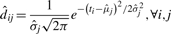
For each group, we first fit a kernel smoother (Venables and Ripley, 2002) to obtain an initial estimate of the number of features and their locations. If the smoother yields a single peak, we estimate the feature parameters as follows:

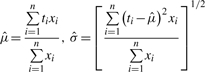To estimate the scale of the feature, we first take the fitted density squared as the weights,

Then assuming multiplicative error,

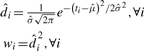
If the smoother has multiple peaks, we use a maximization–expectation (EM) algorithm with pseudo-likelihood for the estimation. Similar to the above, we only consider the likelihood of the observed frequencies. To initiate the algorithm, we first split the group at the valleys of the smoother, and use the data points in each subgroup to obtain the initial estimates of with the equations above, where j denotes the feature. In the following equations, we omit the step number for simplicity. An important difference from the regular EM algorithm is the addition of a third step in every iteration that potentially eliminates some components of the mixture. This is because of the high noise in the data, which could introduce false peaks. Hence in every iteration, we eliminate peaks that explain the data at a percentage that is smaller than a predetermined cut-off level.

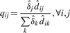
• Step 1, the E step. At every t_i, we find the expected proportions of the observed counts that belong to each component j, denoted q_ij.

  
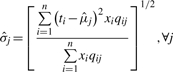
• Step 2, the M step. We find the MLE given the estimated q_ij in the previous E step. For every feature j,

  

  

  

  

  
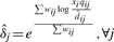
• Step 3, The elimination step. Find the percentage of observed intensities explained by each peak,

  

Remove component j if Q_j is smaller than a threshold. If any component is removed, the above M step is repeated before entering the next iteration.

2.3 Aligning retention time

After Steps 1 and 2, a feature table is generated for every LC/MS profile. The retention time alignment is based on feature-level information. First, features are aligned using their m/z values alone. To align the m/z values, we first search for a lenient m/z tolerance value using the same strategy as described in Section 1. The difference is that feature m/z values, rather than data point m/z values, are used. After grouping the features based on the tolerance level, we fit kernel density to the m/z values within each group. If the density in a group shows multiple modes, we split the group at the valley positions of the density estimate. Features in each group are considered to be aligned with each other at the m/z level. Second, a retention-time cut-off value is found by model-based search. Unlike the m/z measurements, the variability in retention time is much higher within a group of features that correspond to the same metabolite, hence a different algorithm is needed. For features grouped together by m/z values, we find the pairwise retention time difference between all features in the group. The retention-time differences from all groups are then combined. The list of the differences (Δ_i) is made of two components: (i) the differences of retention time between features corresponding to the same metabolite, and (ii) the differences of retention time between features from different metabolites having similar m/z. We approximate the feature location by a uniform distribution. Consequently the (ii) component follows a triangular density function. We first estimate the density of Δ using kernel density estimation. Then a straight line is fitted on the estimated density between d₁ and the maximum retention time. The parameter d₁ is chosen such that it is larger than the normal range of feature groups corresponding to a single metabolite. We determine the threshold by searching for the largest distance value where the observed density is more than 1.5 times that of the fitted value. Each group of features with similar m/z value is then further divided if any of the spacings in retention time is larger than the threshold.

We then select the profile that has the most number of features to be the template, and align all the other profiles against it, one at a time, using a kernel smoother. Only feature groups in which each profile has one and only one feature are selected. Denote the corresponding retention times (τ₁, τ₂, …, τ_n) in the template profile, and (t₁, t₂, …, t_n) in the profile to be aligned. We fit a kernel smoother (τ₁−t₁, τ₂−t₂, …, τ_n−t_n) against (t₁, t₂, …, t_n). We then add the fitted value to (t₁, t₂, …, t_n) to obtain the adjusted retention time. For features with retention time outside the range of (t₁, t₂, …, t_n), their retention times are adjusted with the same amount as the end point t₁ or t_n.

2.4 Aligning features across profiles

After retention time alignment, we repeat the step of model-based search for retention time cutoff and group features accordingly. Within each feature group, we then fit kernel density estimators on m/z and retention time dimensions to potentially further split the group. The final groups represent aligned features across all the profiles. From every group, we take the median m/z and median retention time to be the representative characteristic values for the feature. A table of aligned features is generated, in which median m/z, median retention time, m/z range, and intensities in each profile are recorded for every feature.

2.5 Recovering weaker signals

If a metabolite is not concentrated enough in a sample to pass the run filter, it will not be included in the feature table from that LC/MS profile, leading to a zero entry in the final aligned feature table. However, some valuable information may be lost. With LC-FTMS data, the background noise is in the form of randomly scattered intensities, rather than baseline shift. This allows us to recover the lost information by searching the small region corresponding to features in the aligned feature table. This is done in a conservative manner to reduce the chance of recruiting noise observations as the true signal.

We sequentially open every LC/MS profile. First, an interpolating spline is fit between the retention times of the observed features in the profile and the retention times in the aligned feature table. The retention times in the aligned feature table are adjusted to adapt to the specific profile using this spline in the same manner as in Section 3. Secondly, if a feature in the aligned table has value zero for the profile, we will search a region around the m/z and retention time location of the feature, which is smaller than the region defined by the m/z range and retention time range of this feature across all other profiles. The run filter is not applied in this step. If one or more features are detected, the feature that is most consistent with the parameters in the feature table is taken as the missed feature, and its intensity is put in the aligned feature table to replace the zero value.

3 IMPLEMENTATION AND DISCUSSION

Using the earliermentioned methods, we designed an overall workflow to identify features from profiles, adjust retention times, align features across profiles and recover weak signals (Fig. 4). We implemented the algorithms in an R package named apLCMS (www.sph.emory.edu/apLCMS). The following is a brief description of the major steps. Steps 1 and 2 are single-profile procedures: (i) From CDF format data, group data points, use run filter to reduce noise and select regions in the profile that correspond to features [function: proc.cdf()]; (ii) Identify features from the profile and summarize feature location, spread and intensity [function: prof.to.features()]. The filtered profile can be plotted after Step 1 [function: present.cdf.3d()] (Fig. 5a and b). Steps 3, 4 and 5 are multi-profile procedures: (iii) Retention-time correction across profiles [function: adjust.time()]; (iv) Feature alignment across profiles [function: feature.align()]; (v) Weak-signal recovery [function: recover.weaker()]. A wrapper function [cdf.to.ftr()] is provided such that all the five steps can be conducted by a single line of command in R. All relevant results are returned in a single list object. The central piece of the result is a table with features in the rows and samples in the columns. The user can choose to further analyze the data using R, or export the table to a tab-delimited text file using the write.table() function in a single command line. The operation of the package is file-based, which saves the user from operating the input/output of files. After the user identifies features of interest, the function EIC.plot() can generate plots of extracted ion chrmatograms (Fig. 5c and d). For more details and other diagnostic plots please see the instruction page at http://www.sph.emory.edu/apLCMS/instructions.htm.

Fig. 4.

Workflow of the apLCMS package. Box A, steps for noise removal and feature identification from a single profile; box B, steps for retention time alignment across profiles; box C, steps for feature alignment across profiles.

Fig. 5.

Sample plots by the R package apLCMS. (a) The full profile after square-root transformation of the intensities. (b) A fraction of the profile with cube-root transformation of the intensities showing more details. Relative scale is used for the intensity (z) axis. (c) Plot of the EIC of one feature in eight profiles. (d) Plot of EIC of the same feature in a subset of profiles.

A set of representative profiles were provided by our collaborators. The data belong to a larger biological study, the results of which will be reported separately. For demonstration purposes, eight profiles are used in this paper. They can be downloaded at http://www.sph.emory.edu/apLCMS/sample_data/data1.zip. To study the consistency of feature detection between the profiles, we set the two parameters of the run filter at α = 20 s, and δ = 70%, and allowed a feature to enter the final feature table as long as it was detected in at least one of the profiles. The method detected between 1229 and 1718 features per profile, with a mean of 1566. The average between-profile pair-wise overlap rate (number of overlapping features divided by the average number of features in the two profiles) is 84.4%. Figure 6a shows the detected features from one profile. The feature detection process is illustrated using a small portion of the profile (Fig. 6b). Long ridges along the time axis that represent chemical noise can be filtered out by restraining the spread of the detected features.

Fig. 6.

Illustration of the feature detection. (a) Features detected in a representative LC/MS profile; (b) Illustration of the steps of data point grouping, noise removal and feature detection.

To study the quality of the identified features, we used a more stringent criterion to find features that are consistent across samples. By requiring a feature to be detected in at least four of the eight profiles before weak signal recovery, 880 features were detected. We matched the m/z values of these features against known metabolites using the online service of the Madison Metabolomics Consortium Database (Cui et al., 2008). Two hundred and ninety-five (33.5%) of the features were matched to known metabolites at the tolerance level of 10 ppm, with 121 of them being unique matches (Supplementary Table 1). We examined the matched metabolites for common metabolites. Among the 20 amino acids, 6 (Gln, Ile, Leu, Phe, Trp, Tyr) have m/z matches in the list, while another 9 (Ala, Asn, Cys, Glu, Gly, His, Lys, Ser, Val) have at least one derivative in the list. Because apLCMS separates features with the same m/z but different retention time, we rounded the detected m/z values at the 4th decimal place and found 826 unique m/z values, among which 269 (32.5%) were matched to know metabolites.

As a comparison, we analyzed the same data using the xcms package (Smith et al., 2006). In an effort to optimize the performance, we tuned four parameters of xcms—step (the step size; values tested: 0.1, 0.01, 0.001), mzdiff (minimum difference for features with retention time overlap; values tested: 0.1, 0.01, 0.001), snthresh (signal to noise ratio cutoff; values tested: 10, 6, 3) and max (maximum number of peaks per EIC; values tested: 10, 5). We left the sigma parameter (standard deviation of the matched filter) at the default value because the default is close to the average standard deviation of the features identified by apLCMS. All 54 combinations of the parameters were tested on the same dataset, and the m/z values of the identified features that were present in at least four of the eight profiles were matched against known metabolites using the Madison Metabolomics Consortium Database (Cui et al., 2008). The results are summarized in Supplementary Table 2. The best performing parameter combinations (step = 0.001, mzdiff = 0.1, snthresh = 3, max = 5 or 10) yielded 768 features, 177 (23.1%) of which were matched to known metabolites. At the default parameter setting (first row of Supplementary Table 2), xcms detects 121 in at least four of the eight profiles, 31 (25.6%) of which were matched to known metabolites.

Comparatively, apLCMS identifies more features (880 versus 768). In addition, the features identified by apLCMS were matched to known metabolites at a higher rate (33.5% versus 25.6%). At 10-ppm tolerance level, 59% of the features identified by apLCMS have matched m/z among the features identified by xcms, which is a decent agreement. These findings suggest that apLCMS has higher sensitivity to detect signals. At the same time, apLCMS also shows higher specificity by identifying a higher percentage of features that can be matched to known metabolites.

As one of the most technically advanced software packages that processes LC/MS data, xcms has been criticized for the use of binning in the m/z dimension, which could artificially merge separate features (Aberg et al., 2008). In addition, the matched filter assumes equal spread in retention time for all features. According to our observation, the assumption may be violated in many situations. The use of this kind of techniques is necessary when the background noise is high. In processing highly noisy data, the algorithms have to lean heavily towards high specificity, rather than high sensitivity, to avoid detecting too many false features. However, with newer data that has little background shift and high m/z precision, we can lean towards sensitivity, rather than specificity, in the effort to keep as much true signal as possible, while keeping the specificity at a reasonable level with the help from the good quality of the data. This philosophy guided the development of the apLCMS package.

The apLCMS package relies on several adaptive procedures to avoid hard cutoffs. First, the feature detection is done using a combination of model-based tolerance level search and kernel density-based iterative splitting (Fig. 4, Box A). The goal of this complex scheme is to separate features whose m/z values are very close to each other. Second, the algorithm doesn't force a specific spread level on the features. Rather, the spread is learned from the data. Third, the algorithm allows features that overlap in m/z and partially overlap in retention time to be separated and gives the maximum likelihood estimate of the areas.

In metabolomics studies, a variety of experimental designs are used, from simple case-control to more complex cross-over designs, time series, etc. Some designs require advanced statistical analysis, or even new methods developed specifically for the design. A data preprocessing pipeline embedded in an advanced statistical platform can provide researchers with the convenience of a seamless connection with downstream statistical analysis. In developing the methods, we focused on the data preprocessing aspects of LC/MS data analysis, including noise removal, feature detection, feature quantification and alignment across LC/MS profiles. When internal biochemical standards are available, accurate alignment and quantification of all features, including the standards, can help achieve accurate absolute quantification based on the standards. In a targeted metabolomics study, usually MS/MS is involved, which endows each feature an extra attribute that greatly helps identification. Nonetheless, reliable feature detection/quantification and alignment are still key to the success of such studies, and the methods described here can be adapted relatively easily.

To suit the need of modern large-scale LC/MS metabolomics studies, the R package was designed to preprocess a large number of LC/MS profiles in a single batch. We have tested the package on a batch of over a thousand CDF files, each of which was ∼ 30 Mb in size. The computation time depends on the amount of information contained in the profiles and the parameters. At the default setting, from one CDF file to its feature list, a laptop computer with a core 2 DUO CPU at 2.2 GHz takes around 50 s to detect features from a CDF file that is about 30Mb in size. The package contains a built-in mechanism that is easy to use to speed up computation when multiple CPUs are available. The function cdf.to.feature() saves binary files of noise-removed profiles and feature tables from every CDF file it has finished processing. On each CPU, the user can run the wrapper function on a subset of the CDF files in pre-processing mode. After the preprocessing is (partially) finished, the user can re-run the function on all CDF files. The function will search for the saved binary files in the working directory to save computing time.

It has been argued that if information from different profiles is merged in the stage of feature detection, the detected features will be more reliable. However with large-scale experiments, the sheer size of the data makes it very hard to simultaneously detect features in all profiles. On the other hand, with the high-resolution LC/MS machines, the variability in m/z detected for the same metabolite is quite small across profiles. Thus, we can afford to perform feature detection profile by profile before performing alignment across profiles. The risk from not borrowing information across profiles in feature detection is that some weak signals may be missed. This problem can be alleviated by revisiting profiles and lowering the detection threshold at areas where features are detected in other profiles.

The tolerance-level search algorithm in this paper is designed for the analysis of complex samples, e.g. serum or urine, where a large number of metabolites exist. While the feature detection and quantification will function normally, the model-based search for thresholds and the retention time alignment may break down when there are too few features. However, the R package allows the user to input parameters (tolerance levels) to disable the automatic search, and the functions will be carried out using the user-input parameters. Because the thresholding results are always fine-tuned by non-parametric procedures, the overall package is robust against the selection of the parameters.

REFERENCES

- Aberg KM, et al. Feature detection and alignment of hyphenated chromatographic-mass spectrometric data. Extraction of pure ion chromatograms using Kalman tracking. J. Chromatogr. A. 2008;1192:139–146. doi: 10.1016/j.chroma.2008.03.033. [DOI] [PubMed] [Google Scholar]
- Baran R, et al. MathDAMP: a package for differential analysis of metabolite profiles. BMC bioinformatics. 2006;7:530. doi: 10.1186/1471-2105-7-530. [DOI] [PMC free article] [PubMed] [Google Scholar]
- Bellew M, et al. A suite of algorithms for the comprehensive analysis of complex protein mixtures using high-resolution LC-MS. Bioinformatics. 2006;22:1902–1909. doi: 10.1093/bioinformatics/btl276. [DOI] [PubMed] [Google Scholar]
- Cui Q, et al. Metabolite identification via the Madison Metabolomics Consortium Database. Nat. Biotechnol. 2008;26:162–164. doi: 10.1038/nbt0208-162. [DOI] [PubMed] [Google Scholar]
- Dettmer K, et al. Mass spectrometry-based metabolomics. Mass Spectrom. Rev. 2007;26:51–78. doi: 10.1002/mas.20108. [DOI] [PMC free article] [PubMed] [Google Scholar]
- Du P, et al. Data reduction of isotope-resolved LC-MS spectra. Bioinformatics. 2007;23:1394–1400. doi: 10.1093/bioinformatics/btm083. [DOI] [PubMed] [Google Scholar]
- Hastings CA, et al. New algorithms for processing and peak detection in liquid chromatography/mass spectrometry data. Rapid Commun. Mass Spectrom. 2002;16:462–467. doi: 10.1002/rcm.600. [DOI] [PubMed] [Google Scholar]
- Idborg-Bjorkman H, et al. Screening of biomarkers in rat urine using LC/electrospray ionization-MS and two-way data analysis. Anal. Chem. 2003;75:4784–4792. doi: 10.1021/ac0341618. [DOI] [PubMed] [Google Scholar]
- Katajamaa M, et al. MZmine: toolbox for processing and visualization of mass spectrometry based molecular profile data. Bioinformatics. 2006;22:634–636. doi: 10.1093/bioinformatics/btk039. [DOI] [PubMed] [Google Scholar]
- Katajamaa M, Oresic M. Data processing for mass spectrometry-based metabolomics. J. Chromatogr. A. 2007;1158:318–328. doi: 10.1016/j.chroma.2007.04.021. [DOI] [PubMed] [Google Scholar]
- Lindon JC, et al. Metabonomics in pharmaceutical R&D. FEBS J. 2007;274:1140–1151. doi: 10.1111/j.1742-4658.2007.05673.x. [DOI] [PubMed] [Google Scholar]
- Lu X, et al. LC-MS-based metabonomics analysis. J. Chromatogr. B Analyt. Technol. Biomed. Life Sci. 2008;866:64–76. doi: 10.1016/j.jchromb.2007.10.022. [DOI] [PubMed] [Google Scholar]
- Nobeli I, Thornton JM. A bioinformatician's view of the metabolome. Bioessays. 2006;28:534–545. doi: 10.1002/bies.20414. [DOI] [PubMed] [Google Scholar]
- Nordstrom A, et al. Nonlinear data alignment for UPLC-MS and HPLC-MS based metabolomics: quantitative analysis of endogenous and exogenous metabolites in human serum. Anal. Chem. 2006;78:3289–3295. doi: 10.1021/ac060245f. [DOI] [PMC free article] [PubMed] [Google Scholar]
- Pyke R. Spacings. J. R. Stat. Soc., Series B. 1965;27:395–449. [Google Scholar]
- Robinson MD, et al. A dynamic programming approach for the alignment of signal peaks in multiple gas chromatography-mass spectrometry experiments. BMC Bioinformatics. 2007;8:419. doi: 10.1186/1471-2105-8-419. [DOI] [PMC free article] [PubMed] [Google Scholar]
- Smith CA, et al. XCMS: processing mass spectrometry data for metabolite profiling using nonlinear peak alignment, matching, and identification. Anal. Chem. 2006;78:779–787. doi: 10.1021/ac051437y. [DOI] [PubMed] [Google Scholar]
- Stolt R, et al. Second-order peak detection for multicomponent high-resolution LC/MS data. Anal. Chem. 2006;78:975–983. doi: 10.1021/ac050980b. [DOI] [PubMed] [Google Scholar]
- Sturm M, et al. OpenMS – an open-source software framework for mass spectrometry. BMC Bioinformatics. 2008;9:163. doi: 10.1186/1471-2105-9-163. [DOI] [PMC free article] [PubMed] [Google Scholar]
- Tolstikov VV, et al. Monolithic silica-based capillary reversed-phase liquid chromatography/electrospray mass spectrometry for plant metabolomics. Anal. Chem. 2003;75:6737–6740. doi: 10.1021/ac034716z. [DOI] [PubMed] [Google Scholar]
- Venables WN, Ripley BD. Modern Applied Statistics with S. New York: Springer; 2002. [Google Scholar]
- Wang P, et al. A statistical method for chromatographic alignment of LC-MS data. Biostatistics. 2007;8:357–367. doi: 10.1093/biostatistics/kxl015. [DOI] [PubMed] [Google Scholar]
- Wang W, et al. Quantification of proteins and metabolites by mass spectrometry without isotopic labeling or spiked standards. Anal. Chem. 2003;75:4818–4826. doi: 10.1021/ac026468x. [DOI] [PubMed] [Google Scholar]
- Windig W, Smith WF. Chemometric analysis of complex hyphenated data. Improvements of the component detection algorithm. J. Chromatogr. A. 2007;1158:251–257. doi: 10.1016/j.chroma.2007.03.081. [DOI] [PubMed] [Google Scholar]