Coulombic Effects in Ion Mobility Spectrometry

Abstract

Ion mobility spectrometry (IMS) has been increasingly employed in a number of applications. When coupled to mass spectrometry (MS), IMS becomes a powerful analytical tool for separating complex samples and investigating molecular structure. Therefore, improvements in IMS-MS instrumentation, e.g. IMS resolving power and sensitivity, are highly desirable. Implementation of an ion trap for accumulation and pulsed ion injection to IMS based on the ion funnel has provided considerably increased ion currents, and thus a basis for improved sensitivity and measurement throughput. However, large ion populations may manifest Coulombic effects contributing to the spatial dispersion of ions traveling in the IMS drift tube, and reduction in the IMS resolving power. In this study, we present an analysis of Coulombic effects on IMS resolution. Basic relationships have been obtained for the spatial evolution of ion packets due to Coulombic repulsion. The analytical relationships were compared with results of a computer model that simulates IMS operation based on a first principles approach. Initial experimental results reported here are consistent with the computer modeling. A noticeable decrease in the IMS resolving power was observed for ion populations of >10,000 elementary charges. The optimum IMS operation conditions which would minimize the Coulombic effects are discussed.

Introduction

The ion mobility spectrometry (IMS) has been increasingly used e.g. as a screening tool for narcotics, explosives, and chemical warfare agents [1-5]. Commercial IMS instruments currently provide low resolving powers (less than 40) compared to research grade instruments, which have demonstrated resolving powers in excess of 150 [6, 7]. Though a trade-off in sensitivity is often observed with the research grade IMS instruments, these systems have enabled fast gas-phase separation of compounds such as structural isomers and polymeric conformers. When coupled with mass spectrometers (MS), the hybrid IMS MS instruments provide information on molecular structures within complex mixtures. As the analytical merits of IMS continue to improve, hybrid IMS-MS instrumentation enters the competition with traditional modes of on-line sample fractionation prior to mass analysis [8-10].

Space charge effects in IMS have been the subject of theoretical and experimental studies [11-17]. Early studies recognized that Coulombic interaction can be a significant factor contributing to the IMS peak shape and resolving power [11, 12, 17]. Conditions of negligibly small Coulombic effects in terms of the ion number density were derived [13]. A mathematical formalism describing the ion density distribution, which accounts for Coulombic interactions, was developed [12]. The effects of space charge on the IMS resolution of a miniature ion mobility spectrometer were investigated and relationships for Coulombic expansion have been obtained, assuming that the axial electric field can be roughly approximated as the radial field component in a cylindrical ion packet [14]. Other studies reported that ion densities were insufficient to cause significant electrostatic repulsion effects [13, 15, 16]. After the revised final version of this manuscript was prepared, an ASAP article has become available that uses the SIMION software package [18] to study the effect of space charge in atmospheric pressure IMS systems [19]. In addition to numeric modeling, the publication reports empirical expressions, which predict the ion losses and resolving power as a function of the input charge density and drift tube aspect ratio [19].

Implementation of the ion funnel trap (IFT) has provided considerably increased ion currents, and thus improved sensitivity, dynamic range and throughput of IMS-MS [20-24]. However, such increased ion populations can manifest Coulombic effects that markedly contribute to the spatial dispersion of ions traveling in the IMS drift tube, and thus affecting achievable resolving power. In this report, we present an analysis of the Coulombic effects on IMS resolution for conditions typical for IMS coupled to a time of flight (TOF) MS. We begin with derivation of basic relationships for the spatial evolution of the ion packet due to Coulombic repulsion. The equations obtained are compared to the results of a computer model that simulates IMS operation based on a first principles approach. The theoretical findings are then compared with experimental measurements of ion mobility resolution obtained over a range of pressures and ion populations. Finally, we discuss how these new findings can lead to the optimal IMS configuration.

Methods

Coulombic effects on the spatial dispersion of ions in IMS were evaluated analytically and modeled using a computer simulation approach described in the section “Modeling the ion motion driven by the diffusion and Coulombic field”. The theoretical results were compared with experimental data obtained as follows.

An IMS apparatus used was based upon the design previously reported [24], which utilized an ion funnel trap (IFT) as an ion storage and packet delivery system prior IMS separation. In order to accurately record the total ion current exiting the IMS system and ascertain peak shape, a shielded Faraday plate following the rear ion funnel was used rather than a time-of-flight mass spectrometer (TOF MS). IMS signals were recorded with a Keithley 428 current amplifier operating at a gain of 10⁹ and a rise time filter set up to 100 μs. IMS signal measurements with the Faraday charge collector were also verified in experiments with the IMS instrument coupled to a commercial TOF MS (Agilent, santa Clara, CA). Ions were generated using a custom electrospray configuration [24], in which samples were delivered at a flow rate of 250 nL/min using a needle potential that was 2.5 kV above that of the heated capillary inlet.

Ions were accumulated, stored and injected into the drift tube using the IFT [24]. In an effort to evaluate the proposed model, a sequential range of IFT accumulation times of 1, 2, 4, 8, 16, and 32 ms were used to vary ion populations in the IFT. An ion ejection time of 200 μs ensured nearly complete purging of the IFT after each accumulation event. The ion current information used to evaluate the model was determined by integrating the areas of the analyte peaks of interest in the acquired IMS spectra.

Samples of angiotensin I (Sigma Aldrich, St. Louis, MO) were prepared in a 50:50 methanol:water solution containing 0.1% (v/v) formic acid at concentrations ranging from 100 nM to 5 μM.

Results

1. Spatial evolution of the ion cloud driven by Coulombic repulsion

Generally, thermal diffusion-driven dispersion of ion packets is considered as a primary factor that limits the resolving power of an IMS instrument operating at reduced pressures, while the space charge effects are typically neglected. We begin with an opposite extreme scenario of a very high ion density within the ion packet, such that Coulombic repulsion becomes the dominant factor leading to spatial dispersion of ion packets. Consider an ion cloud having a spherical shape, radius R_q, consisting of a single type of ions having same molecular mass m, charge state z and ion mobility K. The radial expansion of the ion cloud due to Coulombic repulsion is driven by the electric field strength at its surface. According to the Gauss’ law, the field is defined by the surface area of the sphere 4Π R_q² and the total charge contained within this surface, as follows:

$$E_C=Q/\mathit{4}\pi {\epsilon }_{\mathit{0}}{R}_q^{\mathit{2}}$$ (1)

Here Q = ze N_ions is the total charge corresponding to N_ions, the total number of ions in the ion cloud, e is the elementary charge; ε₀ is vacuum permittivity. The electric field E_C is independent of the radial profile of the ion density distribution within the sphere, and is defined by the total charge ze N_ions, as long as spherical symmetry is maintained. The speed of expansion of the outer boundary is determined by the ion mobility. The following differential equation describes the rate of variation of an ion cloud radius as a function of time:

$${\mathit{dR}}_q/\mathit{dt}=K\cdot E_C$$ (2)

After substitution of eq. 1 into eq. 2, the solution is:

$$R_q(t)={\left[\frac{3\mathit{QK}}{4\pi {\epsilon }_0}(t+t_0)\right]}^{1/3}$$ (3)

The constant of integration t₀ can be found from an initial condition of the sphere having radius R₀ in the initial time t = 0:

$$t_0=\frac{4\pi {\epsilon }_0{R}_0^3}{3\mathit{QK}}$$ (4)

The IMS resolution due to Coulombic expansion R_SC can be estimated as the ratio of the drift region length L to the size of the sphere 2C_S R_q. The factor C_S accounts for the full width at half maximum (FWHM) corresponding to the radial number density profile. For the case of a uniformly populated sphere, the coefficient C_S can be estimated based on the z-coordinate, corresponding to the FWHM of the ion density, C_S = 2^-1/2 ≈ 0.71. In the derivation of the ion packet radial dispersion (eq.1-4), we did not make any assumptions on ion density distribution within the sphere R_q(t), except for the spherical symmetry. The uniform density was considered as a possible scenario. Generally, the space charge limited IMS resolution is as follows:

$$R_{\mathit{SC}}=\frac{L}{2C_S{R}_q}=\frac{L}{C_S}{\left(\frac{\pi {\epsilon }_0}{6\mathit{QK\; t}}\right)}^{1/3}$$ (5)

The time t can include the constant t₀, accounting for the initial ion cloud size. Assuming a negligibly small initial ion cloud size, the time t is equal to the IMS drift time:

$$t=\frac{L^2}{\mathit{KV}}$$ (6)

Here V is the voltage drop across the IMS drift region L. The space charge limit to IMS resolving power is then as follows:

$$R_{\mathit{SC}}=\frac{1}{C_S}{\left(\frac{\pi {\epsilon }_0\mathit{LV}}{6Q}\right)}^{1/3}$$ (7)

The relationship accounts for the Coulombic expansion of the ion packet, neglecting the diffusion-driven expansion. We would emphasize that the above derivation of space-charge driven evolution of an ion packet is feasible because of the property of Gauss’ law that defines the radial electric field as a function of the total charge within a specified boundary, independent of ion density distribution. Therefore, our derivation applies to both uniform surface density (i.e., zero volume density) and uniform volume density distributions, and for any other initial density distribution that has a defined boundary R_q. Generally, it can be shown that the ion density distribution inside R_q changes with time, so that the average ion density, defined as the total charge divided by volume, is n_a(t) = ε₀/K(t+t₀).

The diffusion-limited resolving power, neglecting space charge effects and assuming a negligibly small initial ion cloud size, is [17]:

$$R_D={\left(\frac{\mathit{zeV}}{16k_{B}T\ln 2}\right)}^{1/2}$$ (8)

Here k_B is the Boltzmann constant and T is temperature. Both limits show the resolving power increasing with increasing voltage V. R_D is proportional to the square root of voltage, while R_SC is proportional to the cube root of V. The diffusion-limit R_D depends on the ion charge state z and temperature, while the space-charge limit R_SC depends on the drift length L and the total charge Q = ze N_ions. These parameters can be used for an independent optimization of each of the resolving power limits.

Consider, for example, an IMS configuration having V = 1000 V. The diffusion-limited resolving power estimated using eq.8 for z =2 and T =293 K is R_D = 84.5. The space-charge limited resolving power, eq.7, gives R_SC = 201.5 for the ion charge Q corresponding to 10,000 elementary charges, L = 1 m. In this case, the IMS resolution is mainly defined by diffusion, with a minor contribution from Coulombic repulsion. However, at significantly larger (but now obtainable) ion populations, e.g., 1,000,000 elementary charges, a significant space charge contribution results in R_SD = 43.4. Thus, here the two mechanisms produce comparable contributions to the resolving power, and a numerical model accounting for both space charge and diffusion is needed.

2. Modeling the ion motion driven by the diffusion and Coulombic field

The computer model simulated the ion motion in the IMS drift tube, taking into account diffusion and drift motion caused by electric fields. The following equations of ion motion were used:

$$\mathit{dx}=K{E}_{\mathit{Cx}}\mathit{dt}+{\mathit{dx}}_D$$ (9)

$$\mathit{dy}=K{E}_{\mathit{Cy}}\mathit{dt}+{\mathit{dy}}_D$$ (10)

$$\mathit{dz}=K(E+E_{\mathit{Cz}})\mathit{dt}+{\mathit{dz}}_D$$ (11)

where dx, dy, dz are increments of the ion coordinate corresponding to the time step dt, K is the ion mobility, E_Cx, E_Cy, E_Cz are components of the Coulombic field acting on the ion, E, is the drift tube electric field, dx_D, dy_D, dz_D are components of the ion displacement due to diffusion. Diffusion motion was simulated according to the following diffusion motion equation:

$${\mathit{dx}}_D^2+{\mathit{dy}}_D^2+{\mathit{dz}}_D^2=6\mathit{Ddt}$$ (12)

The diffusion coefficient D is related to the ion mobility via Nernst - Einstein equation:

$$D=\frac{k_{B}T}{\mathit{ze}}K$$ (13)

A random number generator was used to generate diffusion increments dx_D, dy_D, dz_D at each time step dt, so that the mean squared displacement equals that defined by eq. 12.

The macro-ion approach [25, 26] was used to calculate the space charge effects caused by Coulombic ion-ion interactions. In this approach, the simulated ion ensemble is represented by a number of macro-ions, N_mi. Each macro-ion is attributed a charge corresponding to a certain number of ions; e. g., 33,000 ions charge state 3+ have the total ion charge 100 Ke, which can be represented in simulations using 1000 macro-ions, each of them having a charge equal to 100 elementary charges. The components of Coulombic electric field E_Cx, E_Cy, E_Cz were calculated as a sum of Coulombic fields from each macro-ion. Computation errors were evaluated using a range of time steps and numbers of macro ions, to ensure that the results converge to a constant value with a desired precision. It was found necessary to use sufficiently small time steps, dt ~ 1·10^-6 s, to accurately model high resolving power conditions. One simulation using 1000 macro-ions took approximately 2 hours using a 2 GHz desktop PC. The computation time increased proportionally to the number of macro-ions squared, which effectively limited this number to ~1000. To obtain a sufficient statistics for modeling the IMS peak shape, repeated simulations were used (up to 100), which resulted in the computation time of > 1 day per one simulated condition, using a desktop PC computer.

3. IMS resolving power due to combined effects of the diffusion and Coulombic expansion

The IMS resolving power was estimated as FWHM of the arrival time distribution (ATD) corresponding to the axial coordinate equal to the drift region length L. This approach agrees with the derivation of eq. 7, with the scaling factor C_S = 2^-1/2. The FWHM definition of the peak width is consistent with the experimental procedure used to determine the IMS resolving power. The ATD was calculated as a histogram of the arrival times obtained in simulations (Figure 1). Two alternative approaches were used to calculate FWHM resolution based on the simulated arrival time data. The first approach used the dispersion of arrival times, Δt_s, calculated as a mean squared deviation of arrival time. It was not necessary to calculate the ATD histogram with this approach, and lower numbers of the arrival time data could be used. This approach was used for fast evaluation of multiple conditions characterized by various pressures and ion charge densities. To relate the dispersion time width, Δt_s, to FWHM values, Δt_FWHM, it was necessary to apply a coefficient

Figure 1.

Arrival time distributions (ATDs) calculated as histograms of the arrival times obtained in simulations. Ion charge is 10,000 e (blue) and 1,000,000 e (red). IMS drift region voltage offset 1000 V. The IMS resolving power was calculated based on the width at half maximum of the ATD peaks. To reduce the statistical noise, the peak profiles were smoothened using the least square fitted modified Gaussian distribution, shown as solid curves.

$$C_{\mathit{HM}}=\frac{\mathrm{\Delta }{t}_{\mathit{FWHM}}}{\mathrm{\Delta }{t}_s}=\sqrt{2\ln 2}$$ (14)

This relationship can be derived based on Gaussian distribution of arrival times [27, 28]. The simulations produced arrival time distributions close to Gaussian, when low ion populations were used, <~50,000 elementary charges, in agreement with the classical theory of the ion mobility. Higher ion populations produced flatter ATD profiles, as illustrated in Figure 1. For such ATDs, the relationship given by eq.14 was inaccurate, and a more direct approach to FWHM calculation is required. Such an approach has been developed based on the arrival time distribution analysis, which mimics experimental determination of the FWHM of a signal trace. The arrival time was binned and the number of occurrences falling within each bin was calculated, to obtain an ATD histogram. The FWHM width of the histogram peak was determined, using interpolation of the histogram values to one half of the maximum. To reduce statistical noise, the peak profile was smoothened using the least square fitted Gaussian distribution. To account for deviations from Gaussian profiles caused by space charge effects, we used polynomials of an order higher than 2, up to 4th order, in the exponent of the distribution function. The histogram-based approach required a larger number of data points compared to the dispersion-based approach, since each histogram bin needed to be populated with a statistically significant count of arrival time data points. A typical simulation used 1000 macro-ions, repeated 10 times to accumulate 10,000 arrival time data points, which provided sufficient population statistics to accurately derive the ATD histograms, as shown in Figure 1.

Figure 2 shows the resolving power calculated for two drift voltages of 1 kV and 4 kV, ion charges ranging from 1000 to 10 million elementary charges (e). Parameters used were: the drift region length L = 1 m, the drift region voltage offset 1 kV (blue curves) and 4 kV (red curves), the drift gas 4 Torr N₂, T = 293 K, ions m = 1000, doubly charged (z = 2), cross section 200 A². Ions were initially distributed uniformly over a sphere of radius R₀ = 1 mm.

Figure 2.

The IMS resolving power for doubly charged ions vs. the ion charge per ion packet, theoretical results. Horizontal axis uses units of millions of elementary charges, Me. Results for two IMS voltages are shown, 1000 V (blue) and 4000 V (red). Horizontal lines: The diffusion-limited resolving power, eq.(8). Dashed curves: the Coulombic IMS resolving power limit, eq.(5) and eq.(7). Solid curves: the IMS resolving power calculated using eq.(16). Symbols: results of the computer modeling. Parameters used for the simulation are: the drift region length L = 1 m, the drift gas 4 Torr N₂, T = 293 K, doubly charged ions (z = 2), m = 1000.

The model was evaluated by comparison with the analytical relationships for the IMS resolving power in the diffusion and space charge limits. The space charge defined limit was calculated using eq. 5, with the time t corrected by the constant of integration t₀, eq. 4, corresponding to the initial radius R₀. It can be seen that under conditions used here the input of t₀ is minor, and eq. 7 produced nearly identical results when neglecting the initial ion packet size.

The diffusion-limited resolving power, eq. 8, is independent of the ion charge, shown by horizontal segments in Figure 2. The modeling produced resolving power values consistent with the analytical relationships. In the limit of low ion population, 1000 elementary charges (e), the modeled resolving power closely approached the diffusion limit. At >10,000 e, the resolving power was noticeably lower than the diffusion limit, e.g. ion populations of 50,000 e produced the resolving power lower by 17% for 1 kV and by 26% for 4 kV. The resolving power reduced by half at 1 million elementary charges (Me) at 1 kV and 0.5 Me using 4 kV. At very high ion population, >~1 Me, the simulation results approached the space charge limit, eq.7, plotted as dashed curves in Figure 2.

Generally, the IMS resolving power accounting for a combined effect of the Coulombic and diffusion-driven expansion can be approximately estimated using a combination of the two limiting relationships. Following a generally used assumption of additive dispersions, e.g., as in the case of Gaussian distributions [27, 28], the combined broadening W_total can be expressed as a function of the diffusional broadening W_diff and Coulombic broadening W_SC:

$$W_{\mathit{total}}=\sqrt{W_{\mathit{diff}}^2+W_{\mathit{SC}}^2}$$ (15)

This relationship can be extended to explicitly account for the broadening due to the initial ion gate pulse width, W_gate. Eq. 15 has been found to be in agreement with the modeling results. However, at pronounced diffusion and space charge effects, the square root relationship, eq.15, produced systematic underestimation of the IMS resolving power by up to ~10%. Better results were obtained using a combination of the cubic powers of the diffusion and Coulombic terms:

$$R_{\mathit{comb}}={\left[R_{\mathit{SC}}^{-3}+R_D^{-3}\right]}^{-1/3}$$ (16)

This relationship accounts for the additive spatial dispersion volumes due to the both mechanisms. The broadening due to the initial ion gate pulse width broadening W_gate can be included in R_SC term similarly to R₀ in eq. 4. Solid curves in Figure 2 were calculated using eq.16, assuming zero initial broadening. A good agreement between the analytical relationship and computer model was obtained.

4. Interaction of multiple ion packets

Considered so far was an idealized case of an ion packet consisting of ion species of the same type, with all ions characterized by same m/z and ion mobility values. In practice, the initial ion packet generally consists of several ion species different in m/z, charge states and ion mobilities. In such a case, the IMS resolving power for a particular ion species is influenced by ion populations of all ion species present in the IMS drift region. A simple case of a multicomponent ion cloud is an ion packet consisting of two ion species. The computer model described above has been modified to include two different ion species. The two ion types begin drifting initially as a single ion packet and then gradually separate into two packets according to ion mobilities of each ion type. The following modeling used a trial ion type, having a fixed ion mobility K₀ and a small ion population of 10⁴ e, mixed with another ion species having a higher ion population of 10⁶ e and the ion mobility coefficient K₁ differing by a factor F_K = K₁ / K₀. The two ion types were initially distributed over the same sphere, radius R₀, as described above for the single-component model.

In the case of two components with ion mobilities differing more than 10%, the resolving power is mostly defined by the low ion population of the trial ion type. If ion mobilities are close, the two ion packets travel together for a longer time, and Coulombic expansion of the smaller component is influenced by the higher ion charge of the other component. Such an interaction of the two packets produces an effect on the IMS peak shape, as demonstrated in Figure 3. In the case of equal ion mobilities, F_K = 1, the peak shape is symmetric and corresponds to a single component ion packet having ~1×10⁶ e charge. For slightly different ion mobilities, F_K = 0.98 and F_K = 1.02, a noticeable asymmetry of the peak shape was observed. In the case of background ions (10⁶ e) having the same ion mobility as the trial ions (10⁴ e), both ion species drift together and the peak shape and resolution of the lower ion charge species is defined by the total ion charge, ~10⁶ e. This is illustrated by the middle distribution in Figure 3 (F_K = 1), which has a profile similar to that of the single component ion cloud (see Figure 1). Other distributions shown in Figure 3 reflect interaction with background ions having ion mobility slightly different than that of the trial ions, 0.98 K₀ and 1.02 K₀. Let us consider the 0.98 K₀ case. The two ion packets partially separate from each other after a certain drift time, so that the higher charge ion packet is on average behind the trial ion packet; space charge field is added to the drift field and the trial ions arrive on average faster. Such a “Coulombic acceleration” explains why the apex of the peak at F_K = 0.98 is shifted towards shorter arrival times, compared to the peak at F_K = 1.0, despite same ion mobility of the trial ions used in both cases. The FWHM broadening is smaller compared to the case F_K = 1, because of the reduced interaction time between two ion clouds. However the baseline width of the peak F_K = 0.98 is close to that at F_K = 1, which can be attributed to the overlapping parts of two ion packets, experiencing on average lower Coulombic acceleration. The other case in Figure 3, F_K = 1.02, can be interpreted similarly and the distribution lineshape was attributed to Coulombic deceleration by the higher space charge ion packet moving at faster velocity than the trial ion packet.

Figure 3.

Arrival time distribution for a small ion population ion packet, 10⁴ e, influenced by a large packet, 10⁶ e, calculated as a histogram of arrival times. Ion mobility ratios of the two ion species are F_K = 1 (diamonds), F_K = 0.98 (squares) and F_K = 1.02 (circles); the small packet charge ions have a fixed ion mobility in all 3 cases. Coulombic expansion of the smaller component is influenced by the higher ion charge of the other component, producing the asymmetric peak shapes, see text. The drift region length L = 1 m, the drift gas 4 Torr N₂, T = 293 K, doubly charged ions (z = 2), m = 1000.

Figure 4a shows the IMS resolving power simulated for the low ion population component of the bi-component ion packet; each point in the plot corresponds to a separate simulation that uses different ion mobility of the background ion K₁. Figure 4b shows the relative deviation of the ion drift time, modeled for the trial low ion population component of the bicomponent ion packet. The drift time of the low abundant component can be changed by as much as 0.4% due to the space charge interaction with the high abundant (10⁶ e) component that has a similar ion mobility. The average drift time data plotted in Figure 4b were obtained as an arithmetic mean of all simulated arrival times, which underestimates the effect of skewed peak shapes, as seen in Figure 3. This implies that slightly higher deviations of the drift time will be obtained if peak maxima are used as a drift time measure, rather then the average time.

Figure 4.

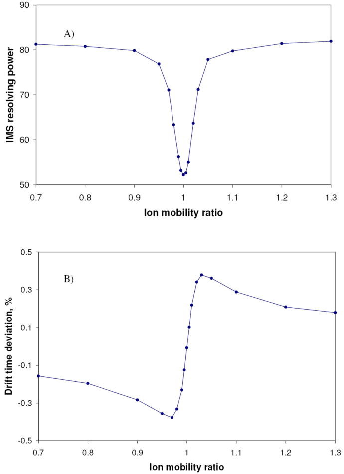
(A) IMS resolving power for a low ion population ion packet, 10⁴ e, influenced by a higher ion population packet, 10⁶ e. The horizontal axis: the ion mobility ratio of the low ion charge and the high ion charge ion species, F_K = K₁ / K₀, see text. (B) Relative deviation of the ion drift time, modeled for the trial low ion population component of the bi-component ion packet. The dispersion based approach for FWHM resolving power was used. Parameters of the model are same as in Figure 3.

A more general scenario of the initial ion packet consisting of multiple ion species is next considered. Here again we calculate IMS resolving power of the trial ion type having a fixed ion population of 10⁴ e and ion mobility K₀. The other ion types are represented by a continuum of ion mobilities evenly distributed in the range 0.5 K₀ to 1.5 K₀, i.e. F_K is in the range 0.5 to 1.5. This scenario qualitatively represents the case of a mixture of many components, e.g. >~100, as encountered in practical analyses of complex mixtures. In this case, the trial ions stay within the axially dispersed ion cloud throughout the period of separation; the resolving power is influenced most during the initial period, when the background ions still hold the initial compact configuration. The resolving power for the trial component is shown in Figure 5; significant effects on resolution occur for background ion populations exceeding ~10⁶ e.

Figure 5.

Simulated IMS resolving power for the trial ion type having a fixed ion population of 10⁴ e, affected by the background ions having a continuum of ion mobilities evenly distributed in the F_K range of 0.5 to 1.5 (see text).

5. Comparison with experimental results

The developed computer model was configured to closely match experimental conditions. An initial ion cloud, at t = 0, was a sphere of radius R₀ = 1mm, uniformly filled with ions. This initial radial size corresponded to the exit orifice of the ion funnel pulser [24]. To account for the ion gate pulse width T_gate, the spherical cloud was extended along z axis over an interval dz₀ = K E_z T_gate. Modeled ion type corresponded to ions used in the experiment, which were angiotensin I at a mass of 1296 Da and a charge state of 3+. The ion mobility K was derived from experimentally observed drift times [24].

Figure 6a, b shows the experimental IMS signals of triply-charged angiotensin I ions at different accumulation times in the ion funnel trap using two different pressure regimes. A general trend observed in experiment was an increase in the analyte signal intensities at longer accumulation times accompanied by the broadening of signal lineshapes. Given a fixed ion gate pulse width and the constant temperature, such signal dispersion could not be explained by thermal diffusion and was attributed to the space charge effect. Drift voltages at different pressures were adjusted to obtain the maximum resolution (i.e., to attain the optimum Townsend’s number E/N, were E is the electric field and N is the gas number density), as evidenced from the ATDs maxima. For each trace in Figure 6, the IMS resolving power was determined as the peak full-width at half-maximum (FWHM) after subtraction of the background level. The IMS resolving power as a function of the ion charge, both measured experimentally and calculated, is plotted in Figures 7a, b. According to the computer model, the space charge effects noticeably degrade resolution starting with ion charges as low as 50,000 elementary charges, the first non-zero ion charge in plots 7a, b. Modeling results were consistent with the experimental data for all pressure and ion charge conditions tested. A coefficient of 0.75 was applied to the experimental ion packet charge data in Figure 7, which improved consistency between the model and experiment. This correction can be attributed, partially, to experimental errors in determining the total ion charge and resolving power from IMS waveforms and, perhaps, imperfect convergence of our modeling results.

Figure 6.

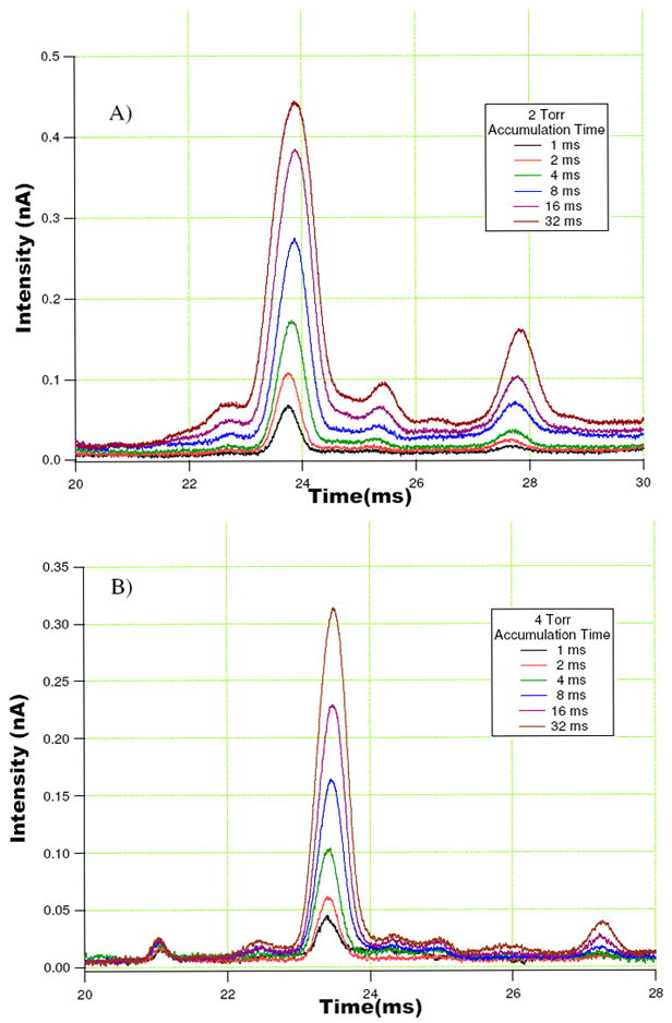
Experimental IMS signals of the triply-charged angiotensin I ions at different accumulation times in the ion funnel trap. IMS operating pressures and drift voltages were: A) 2 torr and 800 V, and B) 4 torr and 1600 V

Figure 7.

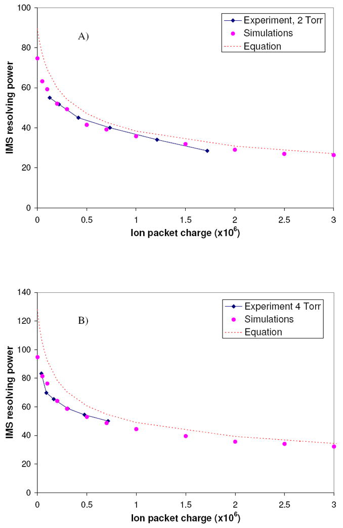
IMS resolving power as a function of. the ion charge, comparison of experimental and theoretical data. (a) p = 2 Torr, V = 800 V (b) p = 4 Torr, V = 1600 V. Diamonds: experimental results; dots: simulations; dotted curves: relationship given by eq.16, which combines the diffusion and Coulombic resolving power limits, and neglects the initial temporal and spatial spreads of an ion packet.

Dotted curves in Figure 7 show the resolving power calculated using the theoretical relationship given by eq.16. The relationship produced trends similar to the modeling and experimental results, with slightly higher resolving powers, which is tentatively attributed to neglecting the initial ion packet size and the gate pulse. This indicates that the resolving power obtained in these experiments was largely determined by the ion packet expansion during the ion motion in the IMS drift region, with a relatively small contribution from the initial conditions, such as the ion pulsing time and the initial ion packet size.

Conclusion

The Coulombic effects on the ion motion in the IMS were analyzed analytically and using a computer model. Relationships have been derived that describe the impact of Coulombic effects on the IMS resolving power. The computer model accounting for diffusion and Columbic repulsion was developed and results were compared to the relationships for the diffusion and space charge limits of the IMS resolving power. The IMS resolving power was calculated for a range of ion populations, using conditions typical for IMS-TOF instruments. The space charge begins to affect IMS resolving power when ion populations are above 10,000 elementary charges, or ~1.6·10^-15 C. Initial experimental results for a range of ion populations and bath gas pressures were found to be in agreement with the theoretical predictions.

Minimization of the Coulombic effects is important for achieving an optimum combination of the high dynamic range and high IMS resolving power. Our analysis shows that the Coulombic limit on resolution increases with increasing IMS voltage, proportionally to the cube root of voltage. This is similar to the classical diffusion limited resolution, which is proportional to the square root of voltage. Thus, increasing the voltage helps to improve the resolution in both cases, but the Coulombic limit increases slower than the diffusion limit. Unlike the diffusion limit, the Coulombic limit also explicitly depends on the drift region length, so that longer drift regions have an advantage.

Initial experimental results indicated that the Coulombically driven ion packet expansion in the IMS drift region for larger ion populations provides a significant contribution to the temporal spread of ions arriving to the detector, compared to the temporal and spatial dispersion of ions at the beginning of IMS separation. We expect that optimizing initial ion cloud size and shape can reduce the space charge effects, when moderate ion populations are used. One possibility is to use initial ion packets extended in the radial direction, to reduce ion number density. Another approach to limit the space charge-driven expansion would be to multiplex ion packet introduction into the IMS drift tube [29-32]. Such an approach reduces the ion charge per packet by creating a series of packets traveling simultaneously in the drift tube.

Along with the increased spatial dispersion, Coulombic repulsion also produces an effect on the average drift velocity of ions within a packet, creating systematic errors in ion mobility measurements. Two ion packets having close ion mobilities interact so that on average the lower mobility component moves slower and vice versa. Our model showed 0.4% drift time deviation caused by the Coulombic repulsion from ions having 10⁶ e charge and close ion mobility values. Further developments of the IMS technology, accounting for the Coulombic effects, should produce improvements in the IMS resolving power and specificity, and improve the overall performance of the technique in analyses of complex systems, such as those studied in proteomics.

References

- 1.Collins DC, Lee ML. Anal Bioanal l Chem. 2002;372:66–73. doi: 10.1007/s00216-001-1195-5. [DOI] [PubMed] [Google Scholar]
- 2.Baumbach JI, Eiceman GA. Appl Spectrosc. 1999;53:338A–355A. doi: 10.1366/0003702991947847. [DOI] [PubMed] [Google Scholar]
- 3.Li F, Xie Z, Schmidt H, Sielemann S, Baumbach JI. Spectrochimica Acta, Part B-Atomic Spectroscopy. 2002;57:1563–1574. [Google Scholar]
- 4.Creaser CS, Griffiths JR, Bramwell CJ, Noreen S, Hill CA, Thomas CLP. Analyst (Cambridge, United Kingdom) 2004;129:984–994. [Google Scholar]
- 5.Kanu AB, Dwivedi P, Tam M, Matz L, Hill HH. J Mass Spectrom. 2008;43:1–22. doi: 10.1002/jms.1383. [DOI] [PubMed] [Google Scholar]
- 6.Wu C, Siems WF, Asbury GR, Hill HH. Anal Chem. 1998;70:4929–4938. doi: 10.1021/ac980414z. [DOI] [PubMed] [Google Scholar]
- 7.Dugourd P, Hudgins RR, Clemmer DE, Jarrold MF. Rev Sci Instrum. 1997;68:1122–1129. [Google Scholar]
- 8.Taraszka JA, Counterman AE, Clemmer DE. Fresenius Journal of Anal Chem. 2001;369:234–245. doi: 10.1007/s002160000669. [DOI] [PubMed] [Google Scholar]
- 9.McLean JA, Ruotolo BT, Gillig KJ, Russell DH. Int J Mass Spectrom. 2005;240:301–315. [Google Scholar]
- 10.Valentine SJ, Plasencia MD, Liu XY, Krishnan M, Naylor S, Udseth HR, Smith RD, Clemmer DE. J of Proteome Research. 2006;5:2977–2984. doi: 10.1021/pr060232i. [DOI] [PubMed] [Google Scholar]
- 11.Spangler GE, Collins CI. Anal Chem. 1975;47(3):403–407. [Google Scholar]
- 12.Watts P, Wilders A. Int J Mass Spectrom Ion Proc. 1992;112(23):179–190. [Google Scholar]
- 13.Spangler GE. Anal Chem. 1992;64:1312–1312. [Google Scholar]
- 14.Xu J, Whitten WB, Ramsey JM. Anal Chem. 2000;72(23):5787–5791. doi: 10.1021/ac0005464. [DOI] [PubMed] [Google Scholar]
- 15.Eiceman GA, Nazarov EG, Rodriguez JE, Stone JA. Rev Sci Instrum. 2001;72:3610–3621. [Google Scholar]
- 16.Spangler GE. Int J Mass Spectrom. 2002;220:399–418. [Google Scholar]
- 17.Mason EA, McDaniel EW. Transport Properties of Ions in Gases. Wiley; New York: 1988. [Google Scholar]
- 18.Dahl DA. Int J Mass Spectrom. 2000;200:3–25. [Google Scholar]
- 19.Mariano AV, Su W, Guharay SK. Anal Chem. 2009 doi: 10.1021/ac802652f. Article ASAP. [DOI] [PubMed] [Google Scholar]
- 20.Tang K, Shvartsburg AA, Lee HN, Prior DC, Buschbach MA, Li FM, Tolmachev AV, Anderson GA, Smith RD. Anal Chem. 2005;77:3330–3339. doi: 10.1021/ac048315a. [DOI] [PMC free article] [PubMed] [Google Scholar]
- 21.Koeniger SL, Merenbloom SI, Valentine SJ, Jarrold MF, Udseth HR, Smith RD, Clemmer DE. Anal Chem. 2006;78(12):4161–4174. doi: 10.1021/ac051060w. [DOI] [PubMed] [Google Scholar]
- 22.Ibrahim Y, Belov ME, Tolmachev AV, Prior DC, Smith RD. Anal Chem. 2007;79(20):7845–7852. doi: 10.1021/ac071091m. [DOI] [PMC free article] [PubMed] [Google Scholar]
- 23.Baker ES, Clowers BH, Li FM, Tang K, Tolmachev AV, Prior DC, Belov ME, Smith RD. J Am Soc Mass Spectrom. 2007;18(7):1176–1187. doi: 10.1016/j.jasms.2007.03.031. [DOI] [PMC free article] [PubMed] [Google Scholar]
- 24.Clowers BH, Ibrahim YM, Prior DC, Danielson WF, Belov ME, Smith RD. Anal Chem. 2008;80(3):612–623. doi: 10.1021/ac701648p. [DOI] [PMC free article] [PubMed] [Google Scholar]
- 25.Tolmachev AV, Kim T, Udseth HR, Smith RD, Bailey TB, Futrell JH. Int J Mass Spectrom. 2000;203:31–47. [Google Scholar]
- 26.Tolmachev AV, Udseth HR, Smith RD. Int J Mass Spectrom. 2003;222(13):155–174. [Google Scholar]
- 27.Siems WF, Wu C, Tarver EE, Hill HH, Jr, Larsen PR, McMinn DG. Anal Chem. 1994;66:4195–4201. [Google Scholar]
- 28.Kanu AB, Gribb MM, Hill HH. Anal Chem. 2008;80:6610–6619. doi: 10.1021/ac8008143. [DOI] [PMC free article] [PubMed] [Google Scholar]
- 29.Clowers BH, Siems WF, Hill HH, Massick SM. Anal Chem. 2006;78:44–51. doi: 10.1021/ac050615k. [DOI] [PubMed] [Google Scholar]
- 30.Szumlas AW, Ray SJ, Hieftje GM. Anal Chem. 2006;78:4474–4481. doi: 10.1021/ac051743b. [DOI] [PubMed] [Google Scholar]
- 31.Belov ME, Buschbach MA, Prior DC, Tang K, Smith RD. Anal Chem. 2007;79:2451–2462. doi: 10.1021/ac0617316. [DOI] [PMC free article] [PubMed] [Google Scholar]
- 32.Belov ME, Clowers BH, Prior DC, Danielson WF, 3rd, Liyu AV, Petritis BO, Smith RD. Anal Chem. 2008;80(15):5873–83. doi: 10.1021/ac8003665. [DOI] [PMC free article] [PubMed] [Google Scholar]