RNAVLab: A virtual laboratory for studying RNA secondary structures based on grid computing technology

Abstract

As ribonucleic acid (RNA) molecules play important roles in many biological processes including gene expression and regulation, their secondary structures have been the focus of many recent studies. Despite the computing power of supercomputers, computationally predicting secondary structures with thermodynamic methods is still not feasible when the RNA molecules have long nucleotide sequences and include complex motifs such as pseudoknots. This paper presents RNAVLab (RNA Virtual Laboratory), a virtual laboratory for studying RNA secondary structures including pseudoknots that allows scientists to address this challenge. Two important case studies show the versatility and functionalities of RNAVLab. The first study quantifies its capability to rebuild longer secondary structures from motifs found in systematically sampled nucleotide segments. The extensive sampling and predictions are made feasible in a short turnaround time because of the grid technology used. The second study shows how RNAVLab allows scientists to study the viral RNA genome replication mechanisms used by members of the virus family Nodaviridae.

1. Introduction

Ribonucleic acid (RNA) is made up of four types of nucleotide bases: adenine (A), cytosine (C), guanine (G), and uracil (U). A sequence of these bases is strung together to form an RNA molecule that, unlike deoxyribonucleic acid (DNA), is often single-stranded. RNA molecules vary greatly in size, ranging from about 20 nucleotide bases in microRNAs to long polymers of over 30,000 bases comprising entire viral genomes [1]. Among the four nucleotide bases, C and G form a complementary base pair by hydrogen bonding, as do A and U and, less frequently, G and U. Although a single-stranded RNA molecule is a linear polymer, it tends to fold back on itself to form a three dimensional (3D) functional structure mostly by pairing between complementary bases. The 3D structure of an RNA molecule is often the key to its function. Because of the instability of RNA molecules, experimental determination of their precise 3D structures is a time consuming and rather costly process. However, useful information about an RNA molecule can be gained from knowing its secondary structure, which refers to the collection of hydrogen bonded base pairs in the molecule. Essentially, all RNA secondary structures are made up of elements that can be classified into two basic categories: stem-loops and pseudoknots (see Fig. 1 ). Both kinds of secondary structure elements have been implicated in important biological processes such as gene expression and regulation for stem-loops [2] and pseudoknots [3], [4]. We also note that in both stem-loops and pseudoknots, it is necessary to have a stretch of nucleotide sequence (ACCGUC in Fig. 1a and b) followed by its inverted complementary sequence (GACGGU) downstream. For simplicity, we shall refer to these kinds of patterns as close inversions. The development of mathematical models and computational prediction algorithms for stem-loop structures based on thermodynamic models started in the 1980s [5], [6]. Pseudoknots, because of the extra base pairings, must be represented by more complex models and data structures. Despite the computing power of supercomputers and emerging advanced technologies, e.g., multi-core architectures, the prediction of secondary structures of long RNA sequences (on the order of thousands of nucleotides) based on thermodynamic methods, e.g. [7], is still not feasible, especially if the structures include complex secondary structures like pseudoknots. The time and space required for accurate predictions of pseudoknots based on energy minimizations grow very rapidly with the sequence length. Fig. 2 shows the time and memory (in logarithmic scale) allocated for the prediction of RNA pseudoknots with various lengths using one of the most accurate prediction programs, Pknots-RE [8]. The algorithm underlying Pknots-RE has a runtime and memory demand in the order of $n^6$ and $n^4$, respectively, where n is the length of the input sequence [8]. The program conducts an exhaustive search for the optimal structure with the lowest free energy and has the capability to predict rather complex structures, even some non-planar structures, for short RNA segments up to 200 nucleotides in length. To overcome the tremendous demand on computing resources needed by pseudoknot prediction, alternative algorithms have been proposed (e.g., Pknots-RG [9], ILM [10], and HotKnots [11]) that tend either to restrict the types of pseudoknots or the length of the secondary structure to be predicted to keep runtime and memory size under control. For instance, the program Pknots-RG [9] limits the types of pseudoknots to simpler structures for longer segments, up to 800 nucleotides. However, a large variety of pseudoknots have been shown to occur in nature. Their omission from computational methods may significantly affect the prediction accuracy. Furthermore, even the simplified programs are not able to predict secondary structures on the order of thousands of nucleotides.

Fig. 1.

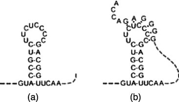
Examples of stem-loop (a) and a pseudoknot (b).

Fig. 2.

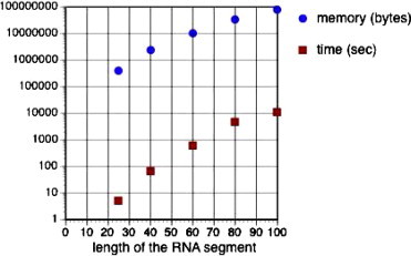
Time (sec) and memory (bytes) used by Pknots-RE for predicting PseudoBase sequences with different lengths.

Our analysis of the length of pseudoknots in a widely used database known as PseudoBase [12], which collects 245 pseudoknots, shows that most pseudoknots known to date are formed by RNA segments whose lengths are less than 200 nucleotides, i.e., 95% of the segments in the database have lengths that range between 20 and 200 nucleotides. The range of lengths between 30 (lower quartile) and 67.5 (upper quartile) nucleotides covers 50% of all segments. This observation leads to the idea of overcoming the computing constraints presented above by developing a strategy for cutting long RNA sequences into segments not longer than 200 bases in length and distributing the task of structure prediction of each segment to be done simultaneously on different computers. Ideally, if two segments that are cut from the same RNA sequence overlap each other, then the predicted structures of their overlapping part should be consistent with one another. Such consistency is important for the final structure assembly. In preliminary work, we observed that arbitrarily cutting the RNA sequence into overlapping segments is not advantageous for consistency. It is well conceivable that when an arbitrary cut goes through the middle of a close inversion, the bases forming the pairings do not get into the same segment, resulting in the omission of the structure from that prediction. For instance, consider a 100 base segment of the Severe Acute Respiratory Syndrome (SARS) coronavirus genome, which is one of the coronavirus genomes analyzed by Chew et al. in [13], from position 25,884 to 25,983 and another segment from position 25,923 to 26,022. When the program Pknots-RE is applied to these segments, two predictions are produced which are shown in Fig. 3 . Note that, over the stretch of the 62 bases that the two segments overlap one another, the two predictions are different. This kind of inconsistency poses a serious problem when the predicted structures of the segments need to be assembled.

Fig. 3.

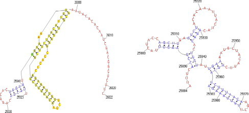
Pknots-RE predictions of two overlapping SARS coronavirus segments, including bases 25,884–25,983 (left) and 25,923–26,022 (right).

If the prediction of secondary structures for long RNA sequences is not feasible with thermodynamic methods even with powerful supercomputers, arbitrarily cutting an RNA sequence into shorter overlapping segments makes the single segment predictions feasible but not advantageous for consistency, unless the cutting algorithm uses the locations of high concentration of close inversions. In addition, once motifs are predicted from sampled segments, they have still to be assembled together into complete secondary structures. Both predictions and rebuilding can significantly benefit from the combined prediction capability of different codes, as opposed to using the single codes separately [14]. Prediction of large numbers of short, overlapping segments is still computationally demanding but it also allows massive task parallelism that can be addressed with grid computing resources. Of course, the scientist who uses such an approach of sampling and rebuilding from segments to predict longer secondary structures has to benefit from the computing capabilities of such a framework without being required to cut and paste results from one code output to another, redirecting or reformatting output files (e.g., from FASTA to EMBL format) before forwarding them to the next step in the analysis, or dealing with distributed computer systems. Therefore, the ideal computing environment for the scientist should integrate key services and functionalities by combining different mechanisms and programs in an automated, computationally powerful, and reliable cyberinfrastructure accessible through an easy-to-use, familiar interface.

These overall needs and key services are integrated in RNAVLab (RNA Virtual Laboratory), a virtual laboratory for the study of RNA secondary structures. RNAVLab addresses the challenges above by combining sampling of nucleotide sequences, predictions based on different codes and supported by grid computing technology, and analysis of large sets of secondary structures with different scientific scopes. Scientific scopes include associating stem-loop and pseudoknot types with functions in genomes. In this paper two important case studies using RNAVLab are presented:

• •To rebuild secondary structures in longer sequences by systematically sampling nucleotide segments from an RNA molecule and assembling the significant motifs found in the secondary structures of the segments (i.e., stem-loops and pseudoknots). The extensive and systematic sampling of nucleotide segments is vital for overcoming the inconsistency outlined above; the computing power needed for the prediction of the numerous segments is provided by grid technology. Motifs are identified in the secondary structures of each segment and assembled in a single structure based on their recurrences and statistical insights.
• •To study the association of stem-loop and pseudoknot structures with the viral RNA replication mechanisms for the genomes of members of the virus family Nodaviridae. In other words, RNAVLab helps scientists to address questions such as “what are the mechanisms of nodavirus RNA replication?”. The association of predicted secondary structure near the 3′ terminus of the RNA2 genome segments from seven members of the nodavirus family with their RNA replication mechanisms is targeted. The nodavirus genomes provide an excellent model system for the study of RNA replication due to their genetic simplicity, the robust yield of RNA replication products, and the ability of the RNAs to replicate in cells from a wide variety of organisms.

The rest of this paper is organized as follows: Section 2 discusses significant related work in the field. Section 3 presents the RNAVLab virtual laboratory and its components. Section 4 shows how to use RNAVLab for rebuilding longer RNA secondary structures from RNA segments and to assist in the study of nodavirus RNA replication. Section 5 concludes and briefly presents future work.

2. Related work

When dealing with RNA secondary structures, scientists have several sources of data and tools available. However, to retrieve pieces of information from these sources as well as to sort and elaborate the data with these tools, scientists have to do significant handwork by sorting, computing, merging, and comparing results as well as extrapolating conclusions. For instance, when dealing with pseudoknots, scientists need to access databases such as PseudoBase [12], which are not always provided with advanced search engines. The data from the database has to be copied into files of different format (e.g., FASTA and EMBL). Ultimately the scientists have to download and install codes on platforms that do not always fully support the code execution. Even if portable, some of these codes require significant amount of computing power that is not always available on the scientist’s PC. An alternative is to submit the retrieved data to portals that provide prediction and visualization functions. However, the portals provide single prediction approaches that force the scientists to find multiple portals for their prediction. Ideally scientists should be led through the different steps by a unified, easy-to-use environment that screens them from database issues providing them with powerful tools for search, prediction, analysis, and visualization.

While past efforts have been focused on increasing prediction accuracy of sequential RNA prediction programs [8], [9] and prediction efficiency has been improved by using massively parallel high performance machines [15] or local clusters [16], not much is known about RNA prediction systems based on grid computing technology (i.e., heterogeneous, volatile computers, ranging from supercomputers to clusters and PCs connected to the Internet, spread out in different locations). Previously, grid technology was applied successfully to protein structure prediction [17], [18] and similar achievements are expected for RNA secondary structure prediction. With their significant computing power, these computing systems allow the scientists to explore larger spaces of RNA secondary structures.

Among the several tools based on thermodynamics that are available for RNA secondary structure predictions and analysis, the Vienna Package [19] is one of the most well-known packages. It consists of a C code library and several stand-alone programs for the prediction and comparison of RNA secondary structures. The stand-alone programs are not integrated in a unified environment and do not address multiple prediction approaches but instead deploy the Zuker algorithm [6]. Therefore, the Vienna Package does not include the prediction and analysis of pseudoknots. Last but not least, the package does not integrate grid technology.

As an alternative to thermodynamic methods for RNA secondary structure prediction, Stochastic Context Free Grammars (SCFG) have been proposed for secondary structure prediction [20]. These approaches rely on estimating probability distributions over a set of transformation rules that define how the fold is formed. SCFGs have the ability to learn the parameters of a generative model by observing a set of sequences with their corresponding secondary structures. In general, SCFGs are outperformed by physics based approaches, although recently Do et al. proposed a generalization of SCFGs where a flexible and richer feature set allows to include free energy parameters more akin to thermodynamic models [21]. However, the complexity of the RNA secondary structures predicted by these methods is restricted by the expressibility of their grammars, thus highly complex structures, such as pseudoknots, cannot be predicted by SCFGs. In addition, the above-mentioned tools are single purpose; they can only be used for secondary structure prediction.

For finding consensus motifs that can be associated with RNA functionalities, most of the previous work takes as input a set of primary sequences and generates as output the set of structural motifs identified, and the differences lie in the search strategy for identifying common motifs. For instance, work presented in [22], [23] uses suffix arrays for efficiently exploring the space of valid secondary structures in their Seed method. In Seed, the search space is constrained by the seed sequence, which is just one of the sequences in the set used to instantiate valid motifs. Seed ranks motifs using a metric that combines the entropy of the segment with the free energy of the secondary structure, as computed by MFOLD [7]. This ranking function reached good results and the top motifs had also the highest Matthews Correlation Coefficient [24]. A drawback of Seed is the fact that it is limited to finding patterns in stem regions only, i.e., no loops or pseudoknots can be identified by the Seed method.

Ashlock and Schonfeld propose a depth annotation scheme to identify common motifs that uses an evolutionary algorithm to cluster folds by projecting them in a two dimensional Euclidean space [25]. This method can identify pseudoknots by assigning a unique identifier to stems. The intuition behind this approach is that similar folds will be placed closer by the projection algorithm. To identify motifs, we need to analyze the output of the projection. Since the method provides a visual representation of the similarity between bricks, it is simple to identify motifs by just looking for clusters. However, as the number of bricks increases, spotting the clusters become less straightforward and we need the help of a clustering algorithm. Another shortcoming of this method is that the distances between the pairs of depth annotations depend on a specific size of segment. Thus prior knowledge of the sequences is needed in order to define an appropriate window size.

There are other approaches to motif finding, see for example [26], but most of them give the desired results provided the secondary structure is not complex (no loops or pseudoknots are included), or provided that we have enough prior knowledge regarding the identity of the motifs. On the contrary, our automated method targets motifs that are as general as possible and exhaustively explores the search space of all the sequences of nucleotides. It is a strictly structural method in the sense that, for the experiments presented here, we only looked at the secondary structure predicted by Pknots-RG. Our preliminary results show that our method can find motifs as simple as small stems and as complex as pseudoknots and loops.

With reference to the deployment of RNAVLab proposed in this paper, to our knowledge, these existing tools have not been used for such an exhaustive survey of the link between RNA secondary structure prediction and nodavirus genome replication. Lastly the highly modular design of RNAVLab makes it easy to add new tools. The tools described above can then be integrated into the array of tools that already exist in RNAVLab.

3. RNAVLab overview

RNAVLab has a modular structure that makes it easy to integrate new features. As shown in Fig. 4 , RNAVLab has three major components: (1) a segment sampler component (Sampling) to sample RNA sequence segments guided by simple heuristics and more sophisticated mathematical methods capable of identifying palindrome distributions; (2) a structure prediction component (Prediction) to predict the structures of the sampled segments using different programs on heterogeneous computers; and (3) a structure analysis component (Analysis) to compare and contrast predictions with observed structures as well as identify similarities and other characteristics across predictions. Each component, described in more detail in this section, is shown in Fig. 5 . RNAVLab also includes a database of pseudoknot structures, PseudoBase++ and an easy-to-use interface; both the database and the interface are also described in this section.

Fig. 4.

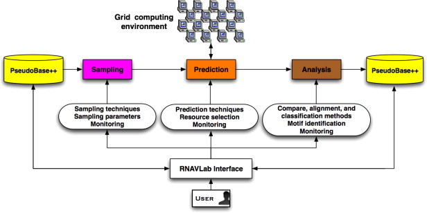
Overview of RNAVLab functionalities, software components, and user interface.

Fig. 5.

Detailed overview of the tools in the three major components of RNAVLab.

3.1. Sampling component

The segment sampler component (Sampling) samples overlapping segments in RNA sequences and passes them to the structure prediction component for the search of significant motifs. Generally, RNA segments containing a high concentration of close inversions have greater tendency to form local secondary structures because the symmetry facilitates base pairing required in the formation of stem-loops and pseudoknots [27], [13]. Currently RNAVLab includes two sampling strategies: a windowing strategy and a progressive segmentation strategy.

In the windowing sampling approach, each set of segments has a fixed size (window size) and a fixed sliding step (window step). The segments in a set are generated by progressively sliding the fixed-size window forward for a fixed number of steps. At each step, the nucleotides within the window form a segment. For an extensive sampling, this procedure is repeated to generate several sets by increasing the window sizes and/or the window steps, each time generating a new set of segments. In our experiments the window sizes are increased by five bases. The maximum length of a window is $n/2$, where n is the length of the RNA sequence we want to rebuild the secondary structure for. Window steps range from 1 base to $w-1$ bases, where w is the window size.

In the progressive sampling approach the user defines a starting point, ending point, and a “step size”; the sampler generates a series of segments by progressively removing “step size” bases from the original segment, whose length is defined by the beginning and ending points (5′ and 3′ termini, respectively) given by the user, starting from the beginning point and progressing in a 5′-to-3′ direction. The series of segments with progressively decreasing lengths are forwarded to the prediction component for prediction. Segments can be inverted before being forwarded. The extension of this component to employ more sophisticated statistics-based sampling methods using the distributional properties of close inversion on random RNA sequences is work in progress.

3.2. Structure prediction component

The structure prediction component (Prediction) harnesses heterogeneous computing resources across the University of Texas at El Paso (UTEP) campus to rebuild RNA secondary structures from the segments generated by sampling, using a variety of prediction programs. Currently RNAVLab supports the following prediction programs: Pknots-RE [8], Pknots-RG [9], and NuPack [28]. The structure prediction component links the segment sampler component to the structure analysis component. Its main functionalities are: (1) to dispatch jobs provided by the segment sampler to available computing resources across the UTEP campus and (2) to identify completed jobs so that results can be forwarded to the structure analysis component.

To setup a grid computing environment, RNAVLab relies on the Condor framework [29], for a variety of reasons. Condor provides all of the functionalities needed to implement a seamless grid layer that allows for faster prediction of RNA secondary structures by harnessing the idle cycles of computers, i.e., workstations and clusters, across the campus. The pool of machines on which RNAVLab is currently relying consists of 23 single-, double-, and quad-processor 32- and 64-bit machines, and while all these machines run Linux (i.e., Fedora, Kubuntu, SuSE), Condor can also be installed on Unix, Windows (e.g., 2000, XP), and Macintosh (OS X) machines, among others. Condor handles all the details of sending executable and data files to computing resources and retrieving the computation results. Furthermore, Condor provides other useful features, such as checkpointing and job migration that only require re-linking the prediction programs used by RNAVLab with Condor libraries. These features can be very helpful, especially with predictions that take a long time: if the application is interrupted, checkpointing saves the computation’s state so it can be resumed later (instead of starting from scratch), and job migration allows a saved state to resume execution in a different machine. RNAVLab successfully re-links Pknots-RE and NuPack, but not Pknots-RG, due to its use of pthreads. Therefore, Pknots-RG cannot use checkpointing and job migration, but it can still be dispatched to the computing resources. Pknots-RG is usually the fastest of all three programs and therefore checkpointing may not be necessary or even helpful.

To interface RNAVLab with Condor and dispatch jobs, an XML file describing the submitted jobs is generated when the user invokes the use of global resources through the RNAVLab interface. Each job consists of a unique identifier, the name of the prediction program to be used (e.g., Pknots-RE, Pknots-RG, and NuPack), and the command-line parameters (i.e., the input files with the RNA sequences). The XML format is converted into a Condor submit file format, and Condor is used to submit the jobs to the pool. Condor also provides the functionality needed to check whether a submitted job has completed execution: this functionality is blocked while the job is running and only returns when the job is completed. Once all the jobs are submitted through Condor, RNAVLab sequentially checks for the completion of jobs. If RNAVLab stalls because a job is not finished, it does not stall the other jobs, since they are already on the queue. Once jobs are completed, their results are forwarded to the structure analysis component and visualized, if required by the user, on the interface. Although the current pool of machines used by RNAVLab consists only of Linux machines, future work includes its extension to clusters available across the campus as well as the integration and support of BOINC (Berkeley Open Infrastructure for Network Computing) [30] to allow researchers to deploy desktop and laptop PCs owned by students or administration personnel outside the campus when these computers are idle. Work in [17] shows that adding idle cycles of PCs significantly increases available computing power.

3.3. Structure analysis component

The structure analysis component (Analysis) evaluates the consistency of the various predictions collected by the structure prediction component. Currently a set of tools allows the end-user to perform secondary structure classifications, comparisons, alignments, and motif identification. In general, a motif is a repeated pattern in a set of sequences of nucleotides (primary structure), or in a set of secondary structures. An innovative aspect of this component is that RNAVLab deals with secondary structure rather than nucleotide sequences for classification, comparison, alignment, and identification. Secondary structures are considered in terms of strings of brackets, i.e., “(” and “)”, “[” and “]”, “{” and “}”, dots “.”, and colons “:”. Two paired nucleotides are represented with a pair of brackets collocated in the string at the same positions as the related nucleotides in the input segment.

With reference to the classification of secondary structures and more in particular of pseudoknots, the PseudoViewer Classification tool deploys the classification of pseudoknots in [31] that clusters them into six different simple types, i.e., H-, HH-, HHH-, HL_out-, HL_in-, and LL_in-type. Note that “H” means hairpin loop, “L” means bulge loop, “in” means internal loop or multiple internal loops, and “out” means external loop or multiple external loops. The tool for classification works on the string of brackets to extract the proper type. Fig. 6 shows the six pseudoknot types.

Fig. 6.

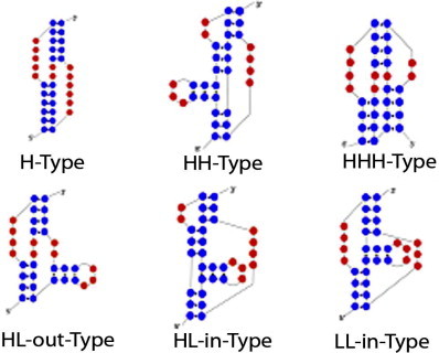
The six pseudoknots types.

Comparisons of observed and predicted structures, or across predicted structures using different programs are performed on aligned or non-aligned strings of brackets. Three different algorithms can be used for comparisons:

• •A variant of the Hamilton algorithm (Hamiltonian Comparison) – the algorithm assigns each kind of nucleotide bond a numerical tag. Bonds GC, CG, UA, and AU are assigned tags from 1 to 4, respectively. The closures of the bonds are all assigned 0. The resulting numerical strings are compared and when two non-zero numbers and their respective closing 0 match, it is counted as a true pair. This approach is useful when the types of nucleotide bonds are important. Fig. 7 shows an example of comparison of a predicted string (Fig. 7a) with an observed string (Fig. 7b) by using the variant of the Hamilton algorithm. The two strings of brackets associated with the prediction and observed secondary structures are converted to two strings of numbers in Fig. 7c. The strings of numbers are compared and the related sensitivity and selectivity are computed. Here, high sensitivity expresses the ability to predict all observed pairs and high selectivity expresses the ability to only predict observed pairs.
• •A stack based algorithm (Comp. Stack) – the algorithm uses stacks to keep track of the positions of open parenthesis and brackets in secondary structures with and without pseudoknots. When an open bracket or parenthesis is encountered, its position is pushed into a stack associated to a stem-loop. Pseudoknots are considered to be a combination of two stem-loops and therefore use two stacks. When a closed bracket or parenthesis is encountered, the position is popped from the associated stack. If a bracket or parenthesis is encountered at the same time in both structures and the position popped from both stacks is the same, this is counted as a true pair. This approach is useful when the identification of exactly alike structures is important. Fig. 8 shows two examples of comparison with this approach: in Fig. 8a the secondary structures are very similar but the bonding nucleotides are shifted and therefore, the comparison has sensitivity and selectivity equal to zero. In Fig. 8b, three bonds in the first string have the same position as three bonds in the second string and this matching results in a higher score for this example in terms of sensitivity and selectivity.
• •A lenient algorithm (Comp. OC – Open–Close parenthesis) – the algorithm uses simple string comparisons that allows for similar yet shifted structures to receive high comparison scores. The algorithm traverses two bracket strings and counts how many times an open bracket or parenthesis is in the same position and how many times a closed bracket or parenthesis is in the same position for the strings, without considering the type of nucleotides involved. The smaller of these two values is the amount of true pairs. Fig. 9 compares the two strings already compared in Fig. 8a with the stack based algorithm. By using the lenient algorithm, higher sensitivity and selectivity are achieved.

Fig. 7.

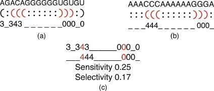
Example of comparison with a variant of the Hamilton algorithm.

Fig. 8.

Example of comparison with a stack based algorithm.

Fig. 9.

Example of comparison with the lenient algorithm.

The alignment of two or more secondary structures is performed by aligning their bracket strings using variants of well-known alignment algorithms such as the Smith–Waterman [32] and Needleman–Wunsch [33] algorithms. Unlike the aforementioned algorithms that align string of nucleotides, i.e., “A”, “U”, “C”, and “G”, the variant algorithms align strings of brackets, i.e., “:”, “(”, and “[”. Shifts are indicated with an underscore, i.e., “_”. The alignment of secondary structure is very important to identify secondary structures that are similar in their shape but are shifted: this can happen when e.g., a predicted structure is compared with an experimentally observed structure or when the genome structures of two viruses belonging to the same family are compared. Fig. 10 shows an example of how the alignment with the variant of the Smith–Waterman algorithm can improve comparison sensitivity and selectivity. Fig. 10a shows the comparison of two strings that have not been a priori aligned; Fig. 10b shows the comparison of the same strings once they have been aligned. The alignment allows for the identification of the two similar structures and affects the sensitivity and selectivity by increasing their final values.

Fig. 10.

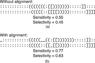
Example of secondary structure alignment.

The Motif Identifier tool performs the identification of common motifs that can be ultimately used for: (1) rebuilding large secondary structures from smaller ones belonging to overlapping RNA segments of the same virus; (2) quantifying the capability of the several prediction programs to capture secondary structures that have been experimentally observed; and (3) classifying unknown viruses by matching common motifs present in their RNA with similar motifs in viruses belonging to a known family. The tool proceeds as follows: first it identifies all the valid secondary structures, from the most simple (e.g., a hairpin comprising a few base pairs) to the most complex (e.g., pseudoknots), that can be generated from the input of secondary structures. Then by using an associative array of linked lists, the tool finds and stores the locations of each substructure generated in the previous step. To narrow down the number of motifs and identify the most relevant ones, ranking techniques are applied. Ranking criteria include: the frequency of the motif over the maximal number of possible occurrences, the number of bonding nucleotides, the length of the secondary structure, and the motif location in the RNA segment. Other possible ranking criteria can include information of the primary structure such as the percentage of bases correctly matched, and/or free energy of the structure as in [34]. In RNAVLab, we score motifs based on their frequency $(f)$, number of base pairs $(s)$, and the length of the overlapping region $(o)$:

$$\text{score}=\frac{f\ast s}{o}\text{.}$$ (1)

The simple intuitive motivation behind this scoring function is that more accurate secondary structures are more likely to be predicted in overlapping segments with higher frequency.

To assemble the significant motifs and rebuild the final secondary structure out of the segment motifs, we use the scoring function above. We project motifs, in descending order according to their score, into a final structure until there are no more mutually exclusive motifs in the set. In other words, we only project different motifs found in segments when they do not overlap with each other. As part of the rebuilding algorithm, we also define the minimum frequency that a motif present in overlapping segments has to meet in order to be projected in the resulting rebuilt sequence (threshold). Threshold values can range from 1 to 9. Finally, we compute the energy of the rebuilt structures as a whole by using the same energy algorithm used in Pknots-RG and NuPack. Fig. 11 shows the pseudocode of the tool.

Fig. 11.

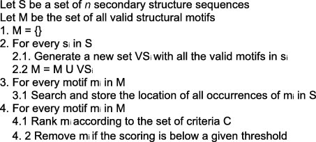
The Motif Identifier algorithm.

In contrast to other approaches for finding common motifs described in Section 2, the Motif Identifier tool finds strictly structural motifs, but it only looks for motifs composed of the folds defined in the initial set: the search space explored is defined by all the valid secondary structures in the set and the tool does not use any information from the primary structures. The algorithm in Fig. 11 was inspired by previous work such as [22], [23], [34]. A key difference is the lack of an ad hoc design: no prior knowledge is assumed about existing motifs and the goal is to discover the motifs that are more likely to be part of the native structure. The algorithm of the Motif Identifier is simple but particularly powerful because it allows identifying complex structures such as pseudoknots. Lastly, since the design is modular new features such as different ranking functions can be easily added. The different tools in the Analysis component can be combined to perform more complex operations on the secondary structures. For instance, motifs that have been identified by the Motif Identifier can be aligned and compared by any of the alignment and comparison tools. Information on the consistency of the prediction results collected can be fed back to the database and made available to the segment sampler component to adjust the sampling strategy and adaptively identify new RNA segments for predictions.

3.4. The database source PseudoBase++

PseudoBase++ (http://pseudobaseplusplus.utep.edu) is part of RNAVLab and includes a database of pseudoknots, a search engine to access the data, and a user interface to select, visualize and insert new data through any web-browser. The database is an extension of PseudoBase [12]: it contains the data related to pseudoknots that is already provided in PseudoBase and other additional data that enriches the information associated to each pseudoknot entry. PseudoBase++ is currently focusing on pseudoknot structures. The primary source of data in PseudoBase++ is PseudoBase: 257 structures are from this database.

3.5. The user interface

The RNAVLab user interface is designed and implemented around the RNAVLab computational environment with a strong focus on compatibility. The implementation idea is also derived from the key concept of encompassing high functionality within a simple but comprehensive interface. By maintaining these two design concepts throughout the process of implementation, the resulting application successfully supports this easy-to-use interface with the rich functionality provided by RNAVLab. The interface is developed in JAVA, thus in nature, preventing any operating system dependencies.

The RNAVLab interface is designed to accommodate the visual structure of a basic media player. This is to create an immediate familiarity for the users as well as maintain a simple comprehensive infrastructure. The interface includes four tabs: database, tools, full results, and previous results. The database tab is a representation of RNA secondary structures in the database. The tools tab is divided into two main sections. One of the sections maintains total functionality with visual representations for the database of sequences, results pertaining to the user’s requests, and previously obtained results. This section is conveniently organized with a tabled panel allowing quick access to any sub-section (Fig. 12 , section on the left). The other main section of the interface provides a constant representation of all concurrent processes being performed by the user as well as a list of each of these processes once they are completed (Fig. 12, section on the right). By selecting any of these processes, the results pertaining to that particular process are displayed conveniently on an information panel located just below in the section on the right in the information window. Though the results are saved and displayed in the full result tab and previous results tab, the visualization in the information window is implemented to allow direct comparisons to several outcomes simultaneously. The interface is capable of supporting two different types of processes through the tools tab, one of sampling and prediction and the other of analysis. Each process has its own convenient selection section with easy checkbox and radio-button options. Each section maintains a copy of the database of sequences with independent sub-lists designated to separate desired sequences or groups of sequences. The first section on the top of the tools tab allows the sampling and prediction with Pknots-RE, Pknots-RG, and NuPack either locally (on the local machine) or globally (across the UTEP campus machines) in accordance to the particular selected sequences or groups of sequences. Reversing and sampling the resulting sequences and classifying the resulting pseudoknot types are also sub-options included in this section. The second section on the bottom of the tools tab allows the user to analyze selected secondary sequences using the tools described in Section 3.3. The tools can be used simultaneously in different combinations.

Fig. 12.

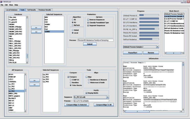
Snapshot of the user interface.

4. Using RNAVLab: two significant case studies

We present two case studies that address the potentials of RNAVLab from two different points of view. In Section 4.1, we present a study in which we address two important analysis components of RNAVLab. First, we quantify its capability to capture the secondary structure observed experimentally. We compare performance and accuracy (in terms of sensitivity and selectivity) of the RNAVLab rebuilding algorithm based on nucleotide segments against a traditional algorithm using the same prediction code and the entire sequence. Second, we statistically quantify the effectiveness of the RNAVLab naive approach for sampling nucleotide segments and we measure whether the extensive sampling and predictions can compensate for the fact that no attention is paid to the type of nucleotides in the segments, i.e., whether or not there are palindromic sequences.

In Section 4.2, we present a second case study in which we show how RNAVLab can be used for studying the correlation between viral RNA replication mechanisms used by members of the nodavirus family and the secondary structures adopted by the 3′ ends of their RNA2 segments, which are hypothesized to play a role in the initiation of complementary strand synthesis during RNA replication.

4.1. Case study I: rebuilding longer RNA secondary structures from motifs in RNA segments

Secondary structures for long RNA sequences i.e., on the order of thousands of nucleotides, that have been experimentally validated are rare. When available, our method can deal with the prediction of these sequences but other methods that predict secondary structures using the entire sequence as a whole cannot, making a comparison between the two approaches infeasible. Therefore, for our analysis in this paper we used the 39 longest nucleotide sequences from Group A in [21] that have lengths ranging from 100 to 482 bases and are still predictable as a whole by the Pknots-RG code. Note that since we are not considering the exact same set as in [21], we cannot perform a direct comparison against those results.

The sampling, motif identification, and rebuilding were executed on the RNAVLab server. Window sizes, window steps, and thresholds used in the experiments are defined in the previous section. The predictions were performed on a 64-node cluster (each node consists of 2 AMD Opteron processors running at 2 GHz with 4 Gbyte of RAM and a local 120 Gbyte hard disk) that is part of the on-campus grid resources of RNAVLab. The accuracy of predictions is measured in terms of sensitivity (i.e., ability to predict all true pairs) and selectivity (i.e., ability to only predict true pairs). Predictions are compared with the experimental secondary structures provided in [21].

Fig. 13 presents the 39 sequences (Sequence), their length in bases (Length), their number of rebuilt structures including those that, when compared with the experimental secondary structures, have sensitivity and selectivity equal to zero (Predictions Attempted), the number of rebuilt structures that have a positive sensitivity and selectivity (Predictions Used), the total time in seconds needed for all the segment predictions on the cluster (Rebuilt Time), and the time in seconds used for the prediction of sequences as a whole when using Pknots-RG (Pred. Time). The figure underlines the high cost in terms of computation needed for our approach. RNAVLab makes our approach feasible by allowing us to perform the computation on idle resources across the campus.

Fig. 13.

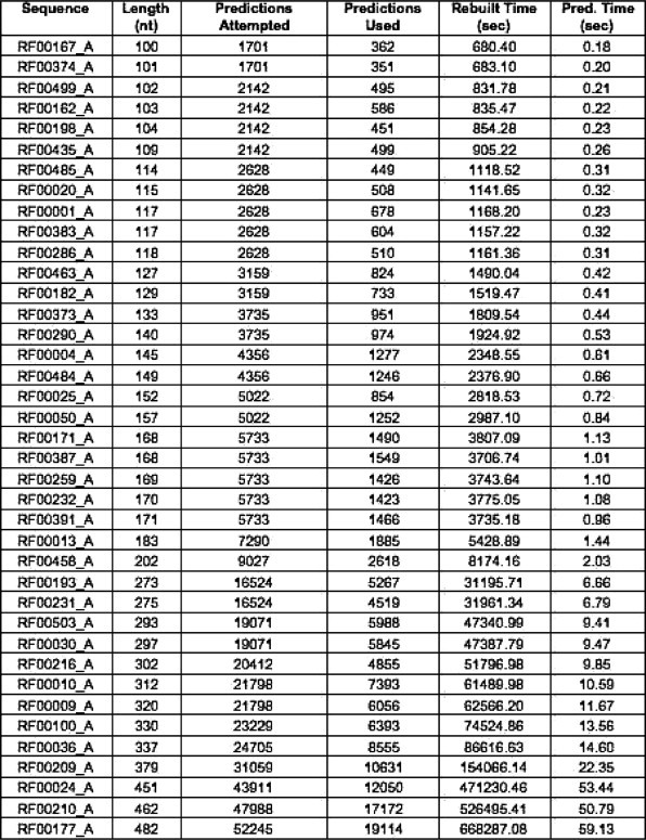
Performance comparison of predictions performed with our rebuilding algorithm based on sampled segments and the same predictions using Pknots-RG and the entire sequence.

4.1.1. Accuracy of rebuilt structures

In Fig. 14 , we present a summary of the accuracies: the oracle or upper bound on sensitivity and selectivity for our method (Rebuilt Sen. and Rebuilt Sel.) is compared with the sensitivity and selectivity of Pknots-RG when considering the entire sequence for prediction (Pred. Sen. and Pred. Sel.) as well as the sensitivity and selectivity achieved by our algorithm when selecting those structures with the lowest free energy (Min En., Min En. Sen., and Min En. Sel.).

Fig. 14.

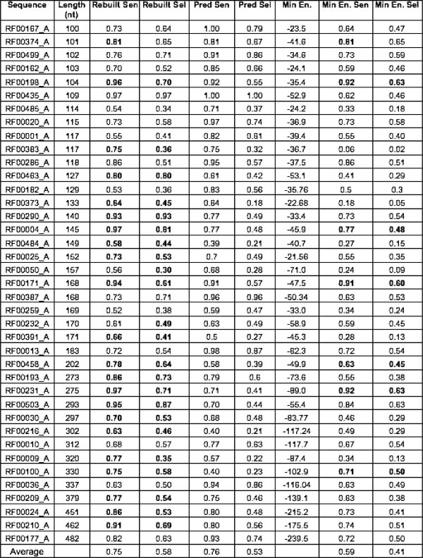
Accuracy comparison (in terms of sensitivity and selectivity) of the upper bound rebuilt predictions based on sampled segments, the same predictions with the entire sequence, and the rebuilt prediction with lowest free energy.

Since we are using Pknots-RG for the prediction of the segments, intuitively we would expect our algorithm to achieve results that are at most equally accurate as those achieved by this prediction code when predicting the whole sequence. However, because we are allowing the prediction of segments starting at different positions in the primary structure, our method can find structures that are very different from those predicted by the code on the entire sequence. Out of the total 39 sequences presented in the figure, the oracle outperformed Pknots-RG on sensitivity and/or selectivity for 24 sequences (see bold values in the figure). However, the selection criteria based on the minimum free energy (Min En. Sen. and Min En. Sel.) are not as accurate: only in 7 out of the 39 cases did these criteria yield better or equal results than Pknots-RG.

The results of our rebuilding algorithm are promising, especially considering the potential of our approach in overcoming the limitations of current prediction methods on the length and complexity of the sequences. Currently, the most salient weakness of our method involves the selection of the final rebuilt structure. The minimum free energy is not by itself a good factor for selection, probably due to what is already common belief that native structures will often be near-optimal in terms of the minimum free energy.

4.1.2. Effectiveness of sampling approach

In cutting an RNA sequence into segments of overlapping sequences, we experimented with various window sizes and window step sizes. In rebuilding the overall structures from the segments, different threshold values were used. We noticed that as values of these parameters vary, the overall accuracy, measured by sensitivity and selectivity of the rebuilt structures, also changes. In order to check whether any significant systematic relationship exists between the accuracy of the rebuilt structures and the parameters, we carried out a multiple regression analysis on each of the 39 sequences in Table 2 with sensitivity and selectivity as response variables and (window size, window step, threshold) as prediction variables.

Table 2.

List of identified common motifs

Virus	Length (nt)	Number of bonds	Frequency	Predictions per code (E, R, N)	Motif
NoV	24	7	0.86	7, 7, 4	(((((((::::::::::)))))))
BBV	15	10	0.83	5, 6, 4	(((((::::)))))
BBV	16	10	0.63	5, 5, 5	(((((::::::)))))
BoV	16	6	1.00	9, 9, 9	((((((::::))))))
BoV	17	5	0.67	5, 1, 7	[[[[[:::::::]]]]]
BoV	56	9	0.56	3, 0, 2	((((:::::))))::::::::::::::::::::::::::[[[[[:::::::]]]]]
BoV	34	11	0.39	4, 0, 3	[[[[[:::::::]]]]]:((((((::::))))))
FHV	14	10	0.78	6, 6, 2	(((((::::)))))
FHV	12	8	0.67	7, 5, 4	((((::::))))
FHV	56	11	0.42	2, 3, 0	[[[[[[:::::::::(((((::::))))):::::::::::::::::::::]]]]]]
FHV	64	9	0.42	2, 3, 0	(((:::::[[[[[[))):::::::::::::::::::::::::::::::::::::::::]]]]]]
FHV	56	6	0.42	2, 3, 0	[[[[[[::::::::::::::::::::::::::::::::::::::::::::]]]]]]
BoV	24	9	0.39	4, 0, 3	((((:::[[[[[)))):::]]]]]
PaV	18	10	0.67	5, 4, 1	((((::::::::))))
PaV	30	7	0.39	4, 1, 2	[[[[:::::::::::]]]]:(((::::)))
PaV	19	4	0.39	4, 1, 2	[[[[:::::::::::]]]]
PaV	26	8	0.33	4, 1, 1	((((:::[[[[:))))::::::]]]]
GGNNV	24	10	0.56	4, 5, 1	(((((:[[[[[))))):::]]]]]
GGNNV	22	5	0.54	8, 4, 1	(((((::::::::::::)))))
GGNNV	41	10	0.50	4, 4, 1	[[[[[::::::::]]]]]:(((((::::::::::::)))))
GGNNV	18	5	0.48	4, 5, 1	[[[[[::::::::]]]]]
SJNNV	21	6	0.83	2, 2, 1	(((:::(((::::)))::)))
SJNNV	42	11	0.50	6, 3, 0	[[[[[::::::::]]]]]((((((::::::::::::))))))
SJNNV	24	10	0.50	6, 3, 0	(((((:[[[[[))))):::]]]]]
SJNNV	24	6	0.43	6, 3, 0	((((((::::::::::::))))))
SJNNV	18	5	0.43	6, 3, 0	[[[[[::::::::]]]]]

In all except one sequence, both sensitivity and selectivity are significantly (p-value <0.005) related to the three prediction variables. Both response variables correlate positively with window size, but negatively with window step and threshold. The positive correlation with window size agrees with our expectation that having a larger sequence segment, which constitutes a larger portion of the whole RNA molecule, in a single prediction should generally be beneficial to the accuracy of the rebuilt structure. On the other hand, a larger window step would mean that successive sequence segments overlap less with each other, so that it is easier to miss those secondary structures spanning both segments but not captured within either one, resulting in the negative correlation with the window step parameter. The negative correlation of threshold with structure accuracy implies that every motif detected in a sequence segment should be taken into account in the rebuilt structure.

A very strong positive correlation between sensitivity and selectivity (correlation coefficient >0.9) has been detected in each of the 39 sequences while the prediction variables are being varied. This suggests that our structure rebuilding approach can be made highly effective simultaneously in both measures of accuracy. It is also interesting to note that the minimum free energy of a rebuilt structure generally shows a negative correlation with sensitivity, but a positive correlation with selectivity, suggesting that the minimum free energy does not necessarily reflect the accuracy of the rebuilt structure. While the minimum free energy is the quantity used pervasively in many secondary structure prediction algorithms for determining the identity of the optimal structure, there seems to be a necessity for seeking an alternative measure.

4.2. Case study II: studying viral RNA genome replication mechanisms for members of the virus family Nodaviridae

For testing the usability of RNAVLab, we considered as our biological system several members of the virus family Nodaviridae collectively known as the nodaviruses, a family of tiny, icosahedral viruses with bipartite, single-stranded RNA genomes. The abundant replication and small genomes of these viruses have made them attractive models for the study of virus structure, virus assembly, and RNA replication. The family Nodaviridae is comprised of two genera: alphanodaviruses and betanodaviruses. While the betanodaviruses have been isolated only from fish, the alphanodaviruses infect predominantly insects; the alphanodavirus Nodamura virus (NoV) also infects mice. Other members of the alphanodavirus genus include Black beetle virus (BBV), Boolarra virus (BoV), Flock House virus (FHV), and Pariacoto virus (PaV). The betanodavirus genus includes many members, including the type species of the genus, Striped jack nervous necrosis virus (SJNNV), and Greasy grouper nervous necrosis virus (GGNNV). These seven viruses were selected here for further study on the basis of the availability of cDNA clones of their genomic RNAs, reagents that will enable us to perform functional assays to determine whether the predicted RNA structures play a role in the viral life cycle. Table 1 shows the abbreviation of the seven viruses, their lengths in terms of nucleotides (nt), and the hosts from which the viruses were isolated, i.e., NoV [35], BBV [36], BoV [37], FHV [38], PaV [39], SJNNV [40], and GGNNV [41].

Table 1.

Selected members of the family Nodaviridae

Virus	Abbrev.	Natural host	Accession number	Length of RNA2 (nt)
Nodamura	NoV	Mosquito, Culex tritaeniorhynchus	NC_002691	1336
Black beetle	BBV	Scarab beetle, Heteronychus arator	NC_002037	1399
Boolarra	BoV	Underground grass grub, Oncopera intricoides	NC_004145	1305
Flock house	FHV	Grass grub, Costelytra zealandica	NC_004144	1400
Pariacoto	PaV	Southern armyworm, Spodoptera eridania	NC_003692	1311
Striped jack nervous necrosis	SJNNV	Striped jack, Pseudocaranx dentex	NC_003449	1410
Greasy grouper nervous necrosis	GGNNV	Greasy grouper, Epinephelus tauvina (Singapore)	NC_004136	1433

The nodavirus genome is divided into two segments of positive-strand RNA: RNA1 encodes the viral RNA-dependent RNA polymerase (RdRp) that replicates both genomic segments, while RNA2 encodes the precursor to the protein that comprises the viral outer coat (capsid) [42]. A small subgenomic RNA3, which is not encapsidated into viral particles, encodes a protein that suppresses host defense mechanisms like RNA interference. During viral RNA replication, the genomic RNA is copied first into a complementary negative strand, which is then used as a template for further positive-strand synthesis. The role of RNA secondary structure in the genome replication of other RNA viruses, e.g., members of the plant tombusvirus, potexvirus, and bromovirus families and the animal picornavirus, coronavirus, and flavivirus families, has been well established in the literature. For example, the RdRp of brome mosaic virus initiates negative strand synthesis at a tRNA-like structure at the 3′ end of the positive-sense RNA template [43]. For the Nodavirus family, Kaesberg et al. [44] had previously used the method of Zuker and Stiegler [45] to perform RNA secondary structure analysis on the 3′ noncoding regions of genomic RNA1 and RNA2 of four nodaviruses (BBV, FHV, NoV, and BoV). This method was able only to predict simple stem-loop structures and not pseudoknots. These authors predicted the presence of stem-loop structures near the 3′ terminus of RNA2 for each of these viruses. However, the cloning and sequencing of three additional nodavirus genomes allowed us to revisit the issue of nodavirus RNA secondary structures and technical advances in the field allow us to test the effect of secondary structure on genome replication in cultured cells. The role of secondary structure on nodavirus RNA replication has been studied previously for only one member, Flock House virus. A long-range interaction between two regions of RNA1 is required for synthesis of subgenomic RNA3 [46]. The results of genetic experiments suggest that a similar long-range interaction may be also required for synthesis of the RNA3 of another member of the family, Nodamura virus (NoV) as well [47]. However, the role of RNA secondary structure in replication of nodavirus genomic RNAs remains unclear. Defining this role is crucial to understanding the mechanism of nodavirus RNA replication. The predictive approaches used in RNAVLab will greatly facilitate our molecular studies by providing a “road map” to elements of possible structural importance, allowing these sequences to be targeted by site-directed mutagenesis.

Previous studies with FHV showed that sequences at the 3′ end of RNA2, particularly within the terminal 50 nucleotides, were critical for RNA replication, and could direct replication of chimeric RNAs that contained heterologous core sequences flanked by RNA2 sequences [48]. By replacing the center of RNA2 with the same heterologous sequence, the work in [48] created a family of RNA molecules that differed only at their termini. The different properties of these molecules could be therefore confidently attributed to these termini. This system established a uniform assay for the different RNAs, using a single probe to the common central core region for Northern blot hybridization experiments. Since such chimeric RNA molecules replicate efficiently, they provide an ideal model substrate for secondary structure prediction and analysis.

4.2.1. Computational results

We used RNAVLab to computationally predict and identify secondary structure motifs in the terminal nucleotides in the 3′ end of RNA2 that could potentially be critical for RNA replication [47]. We analyzed predicted RNA secondary structures of progressively shorter lengths from the 3′ end of RNA2 from the seven members of the nodavirus family presented in Table 1 . Our goal was to identify common motifs across samples, code predictions, and viruses. Due to the dynamic nature of the prediction programs, the final secondary structures are heavily dependent on neighboring structures: having a certain substructure present in all the predictions, independently from the starting and ending points of the segments, may indicate a strong base pairing that ultimately may be present in nature.

For each virus, the terminal 100 nucleotides of the 3′ end of RNA2 were sampled using the progressive segmentation strategy with a step size of 10 nucleotides. The three different prediction programs currently available in RNAVLab were used, i.e., Pknots-RG, Pknots-RE, and NuPack. All the final predictions, obtained from genome segments from different viruses, with different lengths, and different prediction programs, were processed by the tool in the structure analysis component that allows for identifying common motifs, i.e., pseudoknots or stem-loops, and then were aligned for identification of shifted and overlapping structures. The prediction time for the several secondary structures ranged from several hours for long segments predicted using Pknots-RE to a couple of seconds for short segments predicted using Pknots-RG and NuPack. The predictions were performed in parallel across the pool of machines managed by Condor.

For each of the seven viruses, 10 sample segments per virus were processed for prediction using the three codes, for a total of 210 predictions. Within the 210 predictions, 1982 common motifs were found, ranging from simple motif with a single bond to more complex structures such as pseudoknots. To reduce the number of motifs and identify the most significant ones, overlapping motifs were merged into canonical motifs. Overlapping motifs are those contained within larger motifs in terms of nucleotide length and number of bonds but with the same prediction frequency for the same prediction codes and viral genomes. Moreover, simpler motifs, i.e., hairpins with fewer than 4 base pairs, and less frequent motifs, i.e., motifs that were predicted by a single code or had a frequency below 33%, were not considered. The frequency of a motif is measured as the number of times the motif was indeed predicted over the maximum number of times the motif could be predicted by the three codes in samples with a suitable length to accommodate the motif length and its starting portion. This approach reduced the number of common motifs to a set of 28 motifs shown in Table 2 . For each virus, Table 2 presents the motif length, the number of nucleotide bonds, the frequency of the predictions across codes and samples, the number of predictions per code (where E stands for Pknots-RE, R stands for Pknots-RG, and N stands for NuPack), and the motif secondary structures in terms of brackets.

The alignment of the 28 motifs allows for rebuilding larger motifs. Fig. 15, Fig. 16, Fig. 17, Fig. 18, Fig. 19, Fig. 20, Fig. 21 show the output of the RNAVLab analysis (a) and the PseudoViewer representation of the RNA2 terminal part for each virus with the common motif that has resulted from the analysis of the several predictions (b).

Fig. 15.

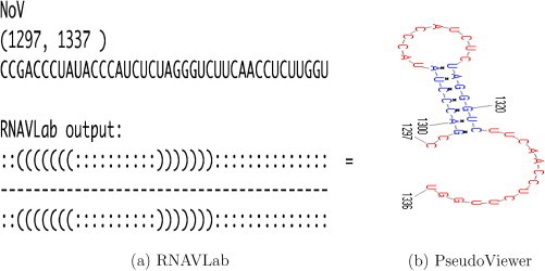
RNAVLab output and PseudoViewer result for NoV.

Fig. 16.

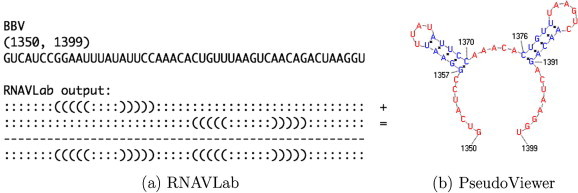
RNAVLab output and PseudoViewer result for BBV.

Fig. 17.

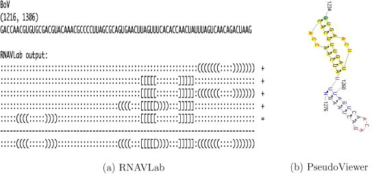
RNAVLab output and PseudoViewer result for BoV.

Fig. 18.

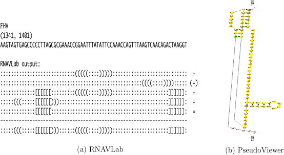
RNAVLab output and PseudoViewer result for FHV.

Fig. 19.

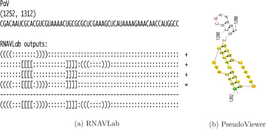
RNAVLab output and PseudoViewer result for PaV.

Fig. 20.

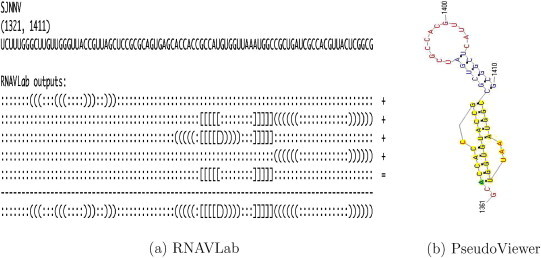
RNAVLab output and PseudoViewer result for SJNNV.

Fig. 21.

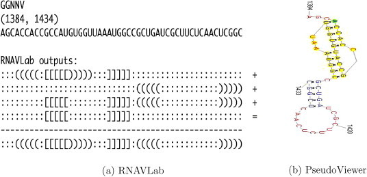
RNAVLab output and PseudoViewer result for GGNNV.

For NoV (Fig. 15) and BBV (Fig. 16), RNAVLab consistently predicts the presence of stem-loop structures near the 3′ end of RNA2. In particular, for NoV a hairpin is predicted from nt 1299 to nt 1322, within the last 50 nucleotides of RNA2. For segments shorter than 40 nucleotides, the stem-loop is no longer predicted. For BBV, we predict two hairpins within the last 50 nucleotides: from nt 1357 to nt 1370 and from nt 1376 to nt 1391, respectively.

For both SJNNV (Fig. 20) and GGNNV (Fig. 21), RNAVLab identifies a pseudoknot followed by a hairpin at the terminal part of their RNA2 segment: while the pseudoknot is identical, the terminal hairpin in SJNNV resembles the hairpin in GGNNV but it has an additional pair of nucleotides. A similar pseudoknot followed by a hairpin is also found at the end of BoV (Fig. 17) and at the terminal part of PaV (Fig. 18), although for the latter virus, this structure is followed by a tail of 23 nucleotides that is predicted to fold into a variety of hairpins of different sizes that vary with the program used. A pseudoknot is found at the very end of FHV (Fig. 19) together with a hairpin that is located inside the pseudoknot to form an HL-out type pseudoknot.

These results found with RNAVLab are consistent with the work conducted experimentally in [48]. We are currently studying whether the pseudoknots and stem-loops are indeed critical structures that drive the genome replication of these viruses. To address this critical question we are combining computational and experimental methods. Driven by the computational results presented in this paper, we will ultimately address the question of whether the biological relevance of the pseudoknots and stem-loops can indeed be experimentally verified. This will be accomplished using two approaches. First, to determine whether the predicted structures can be verified in solution, we will generate a nuclease map using single- and double-strand-specific ribonucleases (RNases) as described by Tuplin et al. in [49]. Viral RNA will be transcribed in vitro and treated with RNases A, T1, and V1, to cleave the 3′ end of single-stranded uracils and cytosines, the 3′ end of single-stranded guanines, and double-stranded nucleotides, respectively. A labeled primer will be used for reverse-transcription of the digested RNAs and sequencing of the undigested cDNA transcription templates. This technique will allow us to confirm or refute predicted structural elements.

Second, to test the role of these predicted structures in the viral life cycle, we will use a process called reverse genetics. Because it is technically difficult to make changes to RNA directly, we will use cloned complementary DNA (cDNA) copies of the viral genomic RNA instead. We will use site-directed mutagenesis to make specific deletions and substitutions of nucleotides within the predicted structural elements. The altered cDNAs will be introduced into cultured cells, where they will be transcribed into RNA by cellular DNA-dependent RNA polymerases. These primary RNA transcripts will then be able to replicate in the presence of the viral RNA-dependent RNA polymerase (RdRp). Therefore, we will test the effect of the RNA2 mutations by transfecting the mutant form into cells together with RNA1 as a source of RdRp. Following incubation to allow the viral RNA to replicate, we will isolate total cellular RNA from the cells and assay for the presence of RNA replication products (negative strand intermediates of RNA1 and RNA2, together with production of subgenomic RNA3) using strand-specific Northern blot hybridization. For example, to test the function of the predicted stem-loop near the 3′ end of NoV RNA2, we could delete it altogether or change specific nucleotides to disrupt base pairing interactions within the predicted stem. If these structures are important for viral RNA replication, we will observe a decrease in the level of replication products detected (relative to wild-type RNA2 controls). Together these methods will allow us to experimentally test whether the structures we predict in the RNAVLab are physically present in the viral RNAs and whether they have functional significance in the viral life cycle.

5. Conclusions and future work

RNAVLab is a virtual laboratory that facilitates the study of RNA secondary structures, i.e., prediction, alignment, comparison, identification, and classification of common secondary structures motifs across viruses, through an automated, computationally powerful approach: the scientist’s intervention is minimized and grid computing technologies are used to address computing intensive tasks such as the prediction of long RNA secondary structures including pseudoknots.

In this paper, RNAVLab is used for rebuilding long secondary structures from significant motifs in RNA segments as well as the computational study of mechanisms that guide RNA replication in the virus family Nodaviridae. For 24 of the 39 RNA sequences with different lengths that we used for the validation of our rebuilding approach, we obtained more accurate (either in terms of sensitivity or selectivity or both) rebuilt structures than those predicted by the same code applied to the whole sequences. The regression analysis results indicated that (1) there is a significant relationship between the accuracy of the rebuilt structure (in terms of sensitivity and selectivity) and the sampling factors (i.e., window size, window step, and threshold values); (2) our method equally targets both the measurements of accuracy, i.e., sensitivity and selectivity; and (3) the minimum free energy cannot be trusted by itself as a quality measure of the secondary structure.

By predicting RNA secondary structures of progressively shorter lengths from the 3′ end on the Nodamura virus RNA2, RNAVLab indicates that, across prediction programs and with different sampled segments, a hairpin structure from nt 1299 to nt 1322 is consistently predicted in the terminal segment of the RNA2 for the Nodamura virus and two hairpins are predicted for the Black beetle virus, from nt 1273 to nt 1286 and from nt 1292 to nt 1307, respectively. These results for NoV and BBV are consistent with the prediction described in [44] except that their prediction included a different fold for BBV nt 1376-1391. Similar secondary structures, i.e., a pseudoknot followed by a hairpin, are predicted in the other members of the family, i.e., Boolarra virus, Pariacoto virus, Striped jack nervous necrosis virus, Greasy grouper nervous necrosis virus. Only in the Flock house virus the pseudoknot includes the hairpin.

Ongoing work includes studying whether the computational findings in both the case studies can indeed be experimentally verified. If this is the case, RNAVLab will be a powerful tool to drive molecular studies by providing a “road map” to elements of possible structural importance, allowing these sequences to be targeted by site-directed mutagenesis.

References

- 1.Thiel V. Mechanisms and enzymes involved in SARS coronavirus genome expression. J. Gen. Virol. 2003;84:2305–2315. doi: 10.1099/vir.0.19424-0. [DOI] [PubMed] [Google Scholar]
- 2.Petrillo M., Silvestro G., Di Nocera P.P., Boccia A., Paolella G. Stem-loop structures in prokaryotic genomes. BMC Genom. 2006;7:170. doi: 10.1186/1471-2164-7-170. [DOI] [PMC free article] [PubMed] [Google Scholar]
- 3.Su M.-C. An atypical RNA pseudoknot simulator and an upstream attenuation signal for −1 ribosomal frameshifting of SARS coronavirus. Nucleic Acids Res. 2005;33(13):4265–4275. doi: 10.1093/nar/gki731. [DOI] [PMC free article] [PubMed] [Google Scholar]
- 4.Wilkinson S.R., Been M.D. A pseudoknot in the 3′ non-core region of the glmS ribozyme enhances self-cleavage activity. RNA. 2005;11:1788–1794. doi: 10.1261/rna.2203605. [DOI] [PMC free article] [PubMed] [Google Scholar]
- 5.Sankoff D. Simultaneous solution of the RNA folding, alignment, and protosequence problems. SIAM J. Appl. Math. 1985;45:810–825. [Google Scholar]
- 6.Zuker M. Computer prediction of RNA structure. Methods Enzymol. 1989;180:262–288. doi: 10.1016/0076-6879(89)80106-5. [DOI] [PubMed] [Google Scholar]
- 7.Zuker M., Mathews D., Turner D. RNA Biochemistry and Biotechnology. Kluwer Academic Publishers; 1999. Algorithms and thermodynamics for RNA secondary structure prediction: a practical guide. [Google Scholar]
- 8.Rivas E., Eddy S.R. A dynamic programming algorithm for RNA structure prediction including pseudoknots. J. Mol. Biol. 1999;285:2053–2068. doi: 10.1006/jmbi.1998.2436. [DOI] [PubMed] [Google Scholar]
- 9.Reeder J., Giegerich R. Design, implementation, and evaluation of a practical pseudoknot folding algorithm based on thermodynamics. BMC Bioinform. 2004;5:104. doi: 10.1186/1471-2105-5-104. [DOI] [PMC free article] [PubMed] [Google Scholar]
- 10.Ruan J., Stormo G.D., Zhang W. ILM: a web server for predicting RNA secondary structures with pseudoknots. Nucleic Acids Res. 2004;32(Web Server issue):W146–W149. doi: 10.1093/nar/gkh444. [DOI] [PMC free article] [PubMed] [Google Scholar]
- 11.Ren J., Rastegari B., Condon A., Hoos H.H. HotKnots: heuristic prediction of RNA secondary structures including pseudoknots. RNA. 2005;11:1494–1504. doi: 10.1261/rna.7284905. [DOI] [PMC free article] [PubMed] [Google Scholar]
- 12.Batenburg van F.H.D. PseudoBase: a database with RNA pseudoknots. Nucleic Acids Res. 2000;28(1):201–204. doi: 10.1093/nar/28.1.201. [DOI] [PMC free article] [PubMed] [Google Scholar]
- 13.Chew D., Choi K., Heidner H., Leung M. Palindromes in SARS and other coronaviruses. INFORMS J. Comput. 2004;16:331–340. doi: 10.1287/ijoc.1040.0087. [DOI] [PMC free article] [PubMed] [Google Scholar]
- 14.T. Estrada, A. Licon, M. Taufer, CompPknots: a framework for parallel prediction and comparison of RNA secondary structures with pseudoknots, in: Proc. First Frontier High Perf. Comp. Network. Workshop, 2006.
- 15.Shapiro B.A. An algorithm for comparing multiple RNA secondary structures. Comput. Appl. Biosci. 1988;4(3):387–393. doi: 10.1093/bioinformatics/4.3.387. [DOI] [PubMed] [Google Scholar]
- 16.Shapiro B.A., Zhang K.Z. Comparing multiple RNA secondary structures using tree comparisons. Comput. Appl. Biosci. 1990;6(4):309–318. doi: 10.1093/bioinformatics/6.4.309. [DOI] [PubMed] [Google Scholar]
- 17.Taufer M. Predictor@Home: a protein structure prediction supercomputer based on global computing. IEEE Trans. Parallel Distrib. Syst. 2006;17(8):786–796. [Google Scholar]
- 18.Zagrovic B., Snow C.D., Shirts M.R., Pande V.S. Simulation of folding of a small alpha-helical protein in atomistic detail using worldwide distributed computing. J. Mol. Biol. 2002;323:927–937. doi: 10.1016/s0022-2836(02)00997-x. [DOI] [PubMed] [Google Scholar]
- 19.Hofacker I.L. Vienna RNA secondary structure server. Nucleic Acids Res. 2003;31(13):3429–3431. doi: 10.1093/nar/gkg599. [DOI] [PMC free article] [PubMed] [Google Scholar]
- 20.Knudsen B., Klein J. RNA secondary structure prediction using stochastic context-free grammars and evolutionary history. Bioinformatics. 1999;15(6):446–454. doi: 10.1093/bioinformatics/15.6.446. [DOI] [PubMed] [Google Scholar]
- 21.Do C.B., Woods D., Batzoglou S. CONTRAfold: RNA secondary structure prediction without physics-based models. Bioinformatics. 2006;22(14):e90–e98. doi: 10.1093/bioinformatics/btl246. [DOI] [PubMed] [Google Scholar]
- 22.T. Nguyen, M. Turcotte, Exploring the space of RNA secondary structure motifs using suffix arrays, in: Proc. Sixth Int. Sympos. Comput. Biol. Genome Inform. (CBGI’05), 2005.
- 23.Anwar M., Nguyen T., Turcotte M. Identification of consensus RNA secondary structures using suffix arrays. BMC Bioinform. 2006;7:244. doi: 10.1186/1471-2105-7-244. [DOI] [PMC free article] [PubMed] [Google Scholar]
- 24.Matthews B. Comparison of the predicted and observed secondary structure of T4 phage lysozyme. Biochim. Biophys. Acta. 1975;(405):442–451. doi: 10.1016/0005-2795(75)90109-9. [DOI] [PubMed] [Google Scholar]
- 25.D. Ashlock, J. Schonfeld, Depth annotation of RNA folds for secondary structure motif search, in: Proc. 2005 IEEE Sympos. Comput. Intell. Bioinf. Comp. Biology, 2005.
- 26.O. Bergig, D. Barash, K. Kedem, RNA motif search using the structure to string method, in: Proc. 2004 IEEE Comp. Syst. Bioinf. Conf., 2004.
- 27.Leung M.-Y. Nonrandom clusters of palindromes in herpesvirus genomes. J. Comput. Biol. 2005;12(3):331–354. doi: 10.1089/cmb.2005.12.331. [DOI] [PMC free article] [PubMed] [Google Scholar]
- 28.N.A. Pierce, NuPack: a software suite for the analysis and design of nucleic acids, 2006. <http://www.nupack.org>.
- 29.Thain D., Tannenbaum T., Livny L. Distributed computing in practice: the Condor experience. Concurr. Comput.: Practice Exp. 2004;17(2–4):323–356. [Google Scholar]
- 30.D.P. Anderson, BOINC: a system for public-resource computing and storage, in: Proc. Fifth IEEE/ACM Int. Workshop Grid Comput. (GRID’04), 2004.
- 31.Han K., Byun Y. PseudoViewer2: visualization of RNA pseudoknots of any type. Nucleic Acids Res. 2003;31:3432–3440. doi: 10.1093/nar/gkg539. [DOI] [PMC free article] [PubMed] [Google Scholar]
- 32.Smith T., Waterman M. Identification of common molecular subsequences. J. Mol. Biol. 1981;147:195–197. doi: 10.1016/0022-2836(81)90087-5. [DOI] [PubMed] [Google Scholar]
- 33.Needleman S.B., Wunsch C.D. A general method applicable to the search for similarities in the amino acid sequences of two proteins. J. Mol. Biol. 1970;48:444–453. doi: 10.1016/0022-2836(70)90057-4. [DOI] [PubMed] [Google Scholar]
- 34.M. Anwar, M. Turcotte, An approach to selecting putative RNA motifs using MDL principle, in: Proc. 2006 Int. Conf. Bioinform. Comput. Biol. (BIOCOMP’06), 2006.
- 35.Scherer W.F., Hurlbut H.S. Nodamura virus from Japan: a new and unusual arbovirus resistant to diethyl ether and chloroform. Am. J. Epidemiol. 1967;86:271–285. doi: 10.1093/oxfordjournals.aje.a120737. [DOI] [PubMed] [Google Scholar]
- 36.Longworth J.F., Carey G.P. A small RNA virus with a divided genome from Heteronychus arator (F.) [Coleoptera: Scarabaeidae] J. Gen. Virol. 1975;33:31–40. doi: 10.1099/0022-1317-33-1-31. [DOI] [PubMed] [Google Scholar]
- 37.Reinganum C., Bashiruddin J.B., Cross G.F. Boolarra virus: a member of the Nodaviridae isolated from Oncopera intricoides (Lepidoptera: Hepialidae) Intervirology. 1985;24:10–17. doi: 10.1159/000149613. [DOI] [PubMed] [Google Scholar]
- 38.Scotti P.D., Dearing S., Mossup D.W. Flock House virus: a nodavirus isolated from Costelytra zealandica (White) (Coleoptera: Scarabaeidae) Arch. Virol. 1983;75:181–189. doi: 10.1007/BF01315272. [DOI] [PubMed] [Google Scholar]
- 39.Zeddam J.-L., Rodriguez J.L., Ravallec M., Lagnaoui A. A noda-like virus isolated from the sweet potato pest Spodoptera eridania (Cramer) (Lepidoptera: Noctuidae) J. Invertebr. Pathol. 1999;74:267–274. doi: 10.1006/jipa.1999.4881. [DOI] [PubMed] [Google Scholar]
- 40.Mori K.-I., Nakai T., Muroga K., Arimoto M., Mushiake K., Furusawa I. Properties of a new virus belonging to Nodaviridae found in larval striped jack (Pseudocaranx dentex) with nervous necrosis. Virology. 1992;187:368–371. doi: 10.1016/0042-6822(92)90329-n. [DOI] [PubMed] [Google Scholar]
- 41.Tan C., Huang B., Chang S.F., Ngoh G.H., Munday B.L., Chen S.C., Kwang J. Determination of the complete nucleotide sequences of RNA1 and RNA2 from greasy grouper (Epinephelus tauvina) nervous necrosis virus, Singapore strain. J. Gen. Virol. 2001;82:647–653. doi: 10.1099/0022-1317-82-3-647. [DOI] [PubMed] [Google Scholar]
- 42.A. Schneemann, L.A. Ball, C. Delsert, J.E. Johnson, T. Nishizawa, Nodaviridae, in: C.M. Fauquet, M.A. Mayo, J. Maniloff, U. Desselberger, L.A. Ball (Eds.), Virus Taxonomy, Eighth Report of the International Committee on Taxonomy of Viruses, Elsevier Academic Press, San Diego, CA, 2005, pp. 865–872.
- 43.Miller W.A., Bujarski J.J., Dreher T.W., Hall T.C. Minus-strand initiation by brome mosaic virus replicase within the 3′ tRNA-like structure of native and modified RNA templates. J. Mol. Biol. 1986;187:537–546. doi: 10.1016/0022-2836(86)90332-3. [DOI] [PubMed] [Google Scholar]
- 44.Kaesberg P., Dasgupta R., Sgro J.-Y., Wery J.-P., Selling B.H., Hosur M.V., Johnson J.E. Structural homology among four nodaviruses as deduced by sequencing and x-ray crystallography. J. Mol. Biol. 1990;214:423–435. doi: 10.1016/0022-2836(90)90191-N. [DOI] [PubMed] [Google Scholar]
- 45.Zuker M., Stiegler P. Optimal computer folding of large RNA sequences using thermodynamics and auxiliary information. Nucleic Acids Res. 1981;9:133–148. doi: 10.1093/nar/9.1.133. [DOI] [PMC free article] [PubMed] [Google Scholar]
- 46.Lindenbach B.D., Sgro J.-Y., Ahlquist P. Long-distance base pairing in Flock House virus RNA1 regulates subgenomic RNA3 synthesis and RNA2 replication. J. Virol. 2002;76:3905–3919. doi: 10.1128/JVI.76.8.3905-3919.2002. [DOI] [PMC free article] [PubMed] [Google Scholar]
- 47.Johnson K.L., Price B.D., Ball L.A. Recovery of infectivity from cDNA clones of Nodamura virus and identification of small nonstructural proteins. Virology. 2003;305:436–451. doi: 10.1006/viro.2002.1769. [DOI] [PubMed] [Google Scholar]
- 48.Albarino C.G. The cis-acting replication signal at the 3′ end of Flock House virus RNA2 is RNA3-dependent. Virology. 2003;311:181–191. doi: 10.1016/s0042-6822(03)00190-9. [DOI] [PubMed] [Google Scholar]
- 49.Tuplin A., Evans D.J., Simmonds P. Detailed mapping of RNA secondary structures in core and NS5B-encoding region sequences of hepatitis C virus by RNase cleavage and novel bioinformatic prediction methods. J. Gen. Virol. 2004;85:3037–3047. doi: 10.1099/vir.0.80141-0. [DOI] [PubMed] [Google Scholar]