Prediction of periventricular leukomalacia. Part II

Summary

Objective

The objective of Part II is to analyze the dataset of extracted hemodynamic features (Case 3 of Part I) through computational intelligence (CI) techniques for identification of potential prognostic factors for periventricular leukomalacia (PVL) occurrence in neonates with congenital heart disease.

Methods

The extracted features (Case 3 dataset of Part I) were used as inputs to CI based classifiers, namely, multi-layer perceptron (MLP) and probabilistic neural network (PNN) in combination with genetic algorithms (GA) for selection of the most suitable features predicting the occurrence of PVL. The selected features were next used as inputs to a decision tree (DT) algorithm for generating easily interpretable rules of PVL prediction.

Results

Prediction performance for two CI based classifiers, MLP and PNN coupled with GA are presented for different number of selected features. The best prediction performances were achieved with 6 and 7 selected features. The prediction success was 100% in training and the best ranges of sensitivity (SN), specificity (SP) and accuracy (AC) in test were 60-73%, 74-84% and 71-74%, respectively. The identified features when used with the DTalgorithm gave best SN, SP and AC in the ranges of 87-90% in training and 80-87%, 74-79% and 79-82% in test. Among the variables selected in CI, systolic and diastolic blood pressures, and pCO₂ figured prominently similar to Part I. Decision tree based rules for prediction of PVL occurrence were obtained using the CI selected features.

Conclusions

The proposed approach combines the generalization capability of CI based feature selection approach and generation of easily interpretable classification rules of the decision tree. The combination of CI techniques with DT gave substantially better test prediction performance than using CI and DT separately.

1. Introduction

In Part I, a companion paper [28], the postoperative hemodynamic and blood gas data of neonates after heart surgery at Children’s Hospital of Philadelphia (CHOP) were used to identify the prognostic factors for the development of PVL through logistic regression (LR) and decision tree (DT) algorithms. Among three cases of datasets - original (without any preprocessing), partial (with only three values from each) and extracted (additional statistical features representing central tendency and distribution over the observation period for each monitoring variable) - Case 3 dataset with extracted statistical features was found better than others for predicting the occurrence of PVL.

Recently, there has been a growing interest in applying data mining and CI techniques in the biomedical domain [1-7]. The techniques include data mining algorithms like DT [8-10], CI based approaches like artificial neural networks (ANNs), fuzzy logic (FL), support vector machine (SVM), genetic algorithms (GA) and genetic programming (GP) [11-20]. Ref. [5] presents a recent review on some of these techniques in clinical prediction. The statistical basis of LR makes it one of the most popular prediction techniques in medical domain. However, the main limitations of LR include the assumption of linear relationship between the independent variables and the logarithm of odds ratio of the dependent variable, and the mandatory dichotomous nature of the dependent variable, which at times restrict the applicability of LR. There are also studies comparing LR and DT for medical domains [9,10]. The main advantages of decision tree (DT) based approach are the ability to handle both continuous and categorical variables, and the generation of classification rules that are easy to interpret. In addition, DT algorithms, being based on the principle of maximizing information-gain, are expected to produce robust models than LR in case of ‘noisy’ or missing data. These features enhance the potential applications of DT in clinical setting [5]. However, the main disadvantage of DT is the poor performance with unknown test data although the training success can be reasonably good. On the other hand, most of the CI techniques have good generalization performance (with reasonably acceptable test success) because of their inherent capability of accommodating complex nonlinear relationships among the independent and the dependent variables. But most CI techniques suffer from the lack of interpretation of the results leading these to be termed as ‘blackbox’ techniques. Another aspect of the commonly used CI techniques is the manual selection of the classifier parameters and the relevant features characterizing the patient/disease condition. In some recent work, the automatic selection of the classifier parameters and the characteristic features has been proposed for diagnosis, monitoring and prognostics of machines and patients, and modeling surface roughness in machining [21-28].

In the present work, the CI based approach of [21-28] is combined with DT to predict the occurrence of PVL. The dataset of extracted statistical features (Case 3 of Part I) was used as inputs to CI based classifiers like multi layer perceptron (MLP) and probabilistic neural network (PNN) in combination with genetic algorithms (GA) for selection of classifier parameters and most suitable features predicting the occurrence of PVL. The selected features were then used as inputs to decision tree induction algorithm for generating rules of classification. The present approach combines the advantages of higher generalization capability of the CI based classifiers and better interpretability of the DT based rules. The present paper is a first attempt to combine CI and DT techniques for identification of potential risk factors in the prediction of PVL occurrence with easily interpretable decision rules. The schematic of the overall procedure is shown in Fig. 1.

Figure 1.

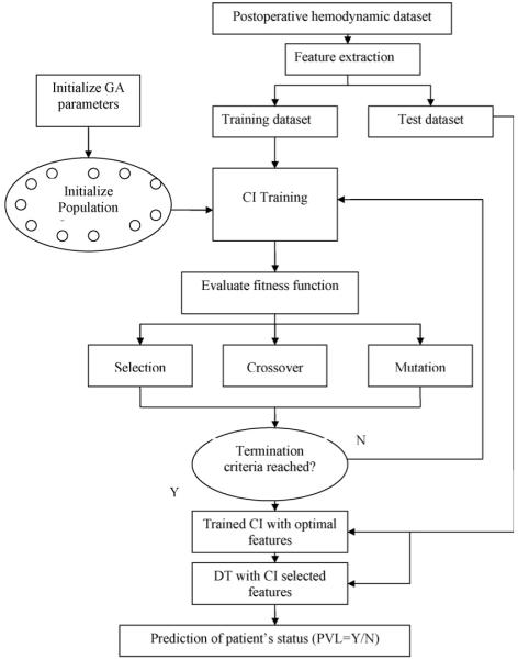
Schematic of CI based process for PVL prediction.

The paper is organized as follows. In Section 2, the CI based methods of MLP and PNN combined with GA are discussed briefly in the context of the present work. Section 3 deals with the selection of features using CI and the correlations among the selected features. The classification results of CI with and without DT are discussed next. The performances of CI and LR in terms of feature selection and PVL prediction are also compared. The conclusions are summarized in Section 4.

2. Computational intelligence (CI) techniques

CI techniques include a number of machine learning, artificial intelligence (AI) and evolutionary algorithms. In this section, two popular categories of ANN along with GA are briefly discussed in the context of the present work.

2.1. ANN

Artificial neural networks (ANNs) have been developed in the form of parallel-distributed network models based on the biological learning process of the human brain. There are numerous applications of ANNs in data analysis, pattern recognition and control [29]. Among different ANNs, two popular types, namely, multi-layer perceptron (MLP) and probabilistic neural networks (PNN) were used for the present work. Brief introductions to MLP and PNN are given here for completeness; readers are referred to texts [29,30] for details.

2.1.1. MLP

MLPs consist of an input layer of source nodes, one or more hidden layers of computation nodes or ‘neurons’ and an output layer. The number of nodes in the input and the output layers depend on the number of input and output variables, respectively. The number of hidden layers and the number of nodes in each hidden layer affect the generalization capability of the network. For a smaller number of hidden layers and neurons, the performance may not be adequate, while with too many hidden nodes, the network may have the risk of over-fitting the training dataset resulting in poor generalization on the new dataset. There are various methods, both heuristic and systematic, to select the number of hidden layers and the nodes [29]. A typical MLP architecture consists of three layers with N, M and Q nodes for input, hidden and output layers, respectively. The input vector x = (x₁, x₂, ..., x_N)^T is transformed to an intermediate vector of ‘hidden’ variables u using the activation function ϕ₁. The output u_j of the jth node in the hidden layer is obtained as follows:

$${\mathsf{u}}_{\mathsf{j}}={\phi }_1(\sum _{\mathsf{i}=1}^{\mathsf{N}}{\mathsf{w}}_{i,j}^1{\mathsf{x}}_{\mathsf{i}}+{\mathsf{b}}_{\mathsf{j}}^1)$$ (1)

where ${\mathsf{b}}_{\mathsf{j}}^1$ and ${\mathsf{w}}_{i,j}^1$ represent respectively the bias and the weight of the connection between the jth node in the hidden layer and the ith input node. The superscript 1 represents the connection (first) between the input and the hidden layers. The output vector y = (y₁, y₂, ..., y_Q)^T of the network is obtained from the vector of intermediate variables u through a similar transformation using activation function ϕ₂ at the output layer. For example, the output of the neuron k can be expressed as follows:

$${\mathsf{y}}_{\mathsf{k}}={\phi }_2(\sum _{\mathsf{i}=1}^{\mathsf{M}}{\mathsf{w}}_{i,k}^2{\mathsf{u}}_{\mathsf{i}}+{\mathsf{b}}_{\mathsf{k}}^2)$$ (2)

where the superscript 2 denotes the connection (second) between the neurons of the hidden and the output layers. There are several forms of activation functions ϕ₁ and ϕ₂, such as logistic function and hyperbolic tangent function given by Eqs. (3) and (4), respectively:

$$\phi \left(\mathsf{v}\right)=\frac{1}{1+{\mathsf{e}}^{-\mathsf{v}}}$$ (3)

$$\phi \left(\mathsf{v}\right)=\frac{1-{\mathsf{e}}^{-2\mathsf{v}}}{1+{\mathsf{e}}^{-2\mathsf{v}}}=\frac{2}{1+{\mathsf{e}}^{-2\mathsf{v}}}-1$$ (4)

The training of an MLP network involves finding values of the connection weights and bias terms which minimize an error function between the actual network output and the corresponding target values in the training dataset. One of the widely used error functions is mean square error (MSE) and the most commonly used training algorithms are based on back-propagation [29].

The feed forward MLP neural network, used in this work, consisted of three layers: input, hidden and output. The input layer had nodes representing the normalized features extracted from the monitored variables of the patients’ biomedical data. The number of input nodes was chosen in the range of 4-7 based on the authors’ related work on the dataset [28]. One output node was used with target values of 1 (0) representing the presence (absence) of PVL. The number of hidden nodes was varied between 10 and 30. In the MLPs, the activation functions of tansigmoid and logistic (log-sigmoid), were used in the hidden and the output layers, respectively. The range of hidden layer nodes and the activation functions were selected on the basis of training trials. The MLP was created, trained and implemented using Matlab neural network toolbox with back-propagation and the training algorithm of Levenberg-Marquardt. The MLP was trained iteratively to minimize the performance function of mean square error (MSE) between the network outputs and the corresponding target values. At each iteration, the gradient of the performance function (MSE) was used to adjust the network weights and biases. In this work, a mean square error of 10^-3, a minimum gradient of 10^-6 and maximum iteration number (epoch) of 100 were used. The training process is designed to stop if any of these conditions were met. The initial weights and biases of the network were generated automatically by the program.

2.1.2. PNN

A PNN consists of many interconnected processing units or neurons arranged in three successive layers after the input layer. The vector x from the input layer is processed in each neuron of the pattern layer to compute its output using a Gaussian spheroid activation function which gives a measure of distance of the input vector from the centroid of the data cluster for each class. The contributions for each class of inputs are summed up to produce a vector of probabilities which allows only one neuron out of the m classes (in the summation layer) to fire with all others in the layer returning zero. The major drawback of using PNNs is the computational cost for the potentially large size of the hidden layer which may be equal to the size of the input vector. The PNN can be Bayesian classifier, approximating the probability density function (pdf) of a class using Parzen windows [30]. The generalized expression for calculating the value of Parzen approximated pdf at a given point x in feature space is given as follows:

$$f_{\mathsf{i}}\left(\mathsf{x}\right)=\frac{1}{{\left(2\pi \right)}^2\sigma {\mathsf{pN}}_{\mathsf{i}}}\sum _{\mathsf{j}=1}^{{\mathsf{N}}_{\mathsf{i}}}{\mathsf{e}}^{-({\mid \mid \mathsf{x}-{\mathsf{x}}_{\mathsf{ij}}\mid \mid }^2∕2{\sigma }^2)}$$ (5)

where p is the dimensionality of the feature vector x, N_i the number of examples of class C_i used for training the network, x_ij represents the neuron vector in the pattern layer, i = 1, m, m being the total number of classes in the training dataset. The parameter σ represents the spread of the Gaussian function and has significant effects on the generalization of a PNN. The probability that a given sample belongs to a given class C_i can be calculated in PNN as follows:

$$\mathsf{p}\left({\mathsf{C}}_{\mathsf{i}}\mathsf{x}\right)=f_{\mathsf{i}}\left(\mathsf{x}\right){\mathsf{h}}_{\mathsf{i}}$$ (6)

where h_i represents the relative frequency of the class C_i within the whole training dataset. The expressions of (5) and (6) are evaluated for each class C_i. The class returning the highest probability is taken as the correct classification. The main advantages of PNNs are faster training and its probabilistic output based on Bayesian statistics. The width parameter (σ) in Eq. (5) is generally determined using an iterative process selecting an optimum value on the basis of the full dataset. However, in the present work the width is selected along with the relevant input features using the GA based approach, as in case of MLPs. The PNNs were created, trained and tested using Matlab.

2.2. Genetic algorithms

GAs have been considered with increasing interest in a wide variety of applications. GAs represent a class of stochastic search procedures based on the principles of natural genetics and through simulated evolution process on a constant-size population of possible solutions in the search space. Each individual member of the population is represented by a string known as genome [31]. The genomes could be binary or real-valued numbers depending on the nature of the problem. In this study, real-valued genomes have been used. The standard GA implementation involves the following issues: genome representation, creation of an initial population of individuals, fitness evaluation, selection of individuals, creation of new individuals using genetic operators like crossover and mutation, and specifying termination criteria. Readers are referred to [31] for details. The basic issues of GAs, in the context of the present work, are briefly discussed in this section.

GA was used to select the most suitable features and one variable parameter related to the particular classifier: the number of neurons in the hidden layer for MLP and the radial basis function (RBF) kernel width (σ) for PNN. For a training run needing N different inputs to be selected from a set of Q possible inputs, the genome string (g) would consist of N + 1 real numbers given in the following equation:

$$\mathsf{g}={\{{\mathsf{g}}_1{\mathsf{g}}_2\cdots {\mathsf{g}}_{\mathsf{N}}{\mathsf{g}}_{\mathsf{N}+1}\}}^{\mathsf{T}}$$ (7)

The first N integers (g_i, i = 1, N) in the genome are constrained to be in the range 1 ≤ g_i ≤ Q. The last number. The last g_N+1 has to be within the range S_min ≤ g_N+1 ≤ S_max. The parameters S_min and S_max represent respectively the lower and the upper bounds on the classifier parameter. In the present work, number of selected features was in the range of 4-7 (N). For MLP, the number of neurons in the hidden layer (M) was taken in the range of 10 (S_min) and 30 (S_max). For PNN, the range of kernel width was taken as 0.10 (S_min) and 3.0 (S_max). A population size of 100 individuals was used starting with randomly generated genomes. A probabilistic selection function, namely, normalized geometric ranking [31] was used such that the better individuals, based on the fitness criterion in the evaluation function, have a higher chance of being selected. Non-uniform-mutation function using a random number for mutation based on current generation and the maximum generation number, among other parameters was adopted. A heuristic crossover was chosen based on the fitness information producing a linear extrapolation of two individuals. The maximum number of generations (100) was adopted as the termination criterion for the solution process. The classification success for the training data was used as the fitness criterion in the evaluation function.

3. Results and discussion

CI techniques were used to select features for prediction of PVL incidence. The dependences of ‘predictors’ were investigated through statistical correlation analyses. Next, CI selected features were used as inputs to a DTalgorithm for generating the decision rules of PVL prediction. The results of CI based approach were compared with DT and LR.

3.1. Prediction results of CI based classifiers

The datasets of normalized features were used for training and testing CI based classifiers, namely, MLP and PNN. Genetic algorithm (GA) was used to select the most important features from the feature pool and the classifier parameters, e.g., the number of neurons in the hidden layer for MLP and the RBF width (σ) for PNN. Study was carried out to see the effect of the number of selected features on the prediction performance. Each classifier was trained using the training dataset and the prediction performance was assessed using the test dataset which was not part of the training process. Table 1 shows the best results for 4-7 selected features over a number of trials. In each case, the training success was 100%. For MLP, the ranges for test sensitivity (SN), specificity (SP) and accuracy (AC) were 47-73%, 68-84%, 68-74%, respectively. For PNN, the ranges of test SN, SP and AC were 60-80%, 63-84% and 71-74%, respectively. For both classifiers, the overall performance (AC) improved with increased number of features with similar performance for 6 and 7 selected features (listed in Table 2(a) and (b)). Most of the selected features were from the same monitoring variables, e.g., diastolic blood pressure (DBP), systolic blood pressure (SBP) and partial pressure of carbon dioxide (pCO₂), although there were some variations in the details of the statistical features. For example, average values of DBP and pCO₂ (DBP_avg and pCO_2avg), and SBP_max were selected by both classifiers. Similarly, pCO₂ was identified in both classifiers with maximum (pCO_2max) in MLPand admission and minimum values (pCO_2adm and pCO_2min) in PNN. The significance of the identified variables is discussed in the following sections.

Table 1.

Prediction results for different CI classifiers

Classifier	No of features	Test success (%)
		SN	SP	AC
MLP	4	47	84	68
	5	73	68	71
	6	73	74	74
	7	60	84	74
PNN	4	80	63	71
	5	67	74	71
	6	60	84	74
	7	73	74	74

Table 2.

Correlation of predictors (a) MLP and (b) PNN

		SBPmax	DBPavg	DBPkrt	RAPskw	pHskw	pCO2max	pCO2avg
(a) MLP
SBPmax	Pearson correlation	1	.545**	-.019	.064	-.067	.056	.284**
	Sig. (two-tailed)		.000	.847	.522	.502	.571	.004
DBPavg	Pearson correlation		1	-.057	.199*	-.158	-.236*	-.102
	Sig. (two-tailed)			.570	.044	.111	.016	.305
DBPkrt	Pearson correlation			1	-.111	-.151	.120	.026
	Sig. (two-tailed)				.265	.128	.226	.797
RAPskw	Pearson correlation		Symmetric		1	.019	-.083	-.030
	Sig. (two-tailed)					.848	.407	.761
pHskw	Pearson correlation					1	-.033	.108
	Sig. (two-tailed)						.739	.278
pCO2max	Pearson correlation						1	.731**
	Sig. (two-tailed)							.000
pCO2avg	Pearson correlation							1
	Sig. (two-tailed)
		HRadm	SBPmax	SBPavg	DBPavg	pCO2adm	pCO2min	pCO2avg
(b) PNN
HRadm	Pearson correlation	1	.200*	.161	.099	.180	.027	-.073
	Sig. (two-tailed)		.043	.104	.322	.069	.788	.463
SBPmax	Pearson correlation		1	.885**	.545**	.178	.358**	.284**
	Sig. (two-tailed)			.000	.000	.073	.000	.004
SBPavg	Pearson correlation			1	.538**	.193	.348**	.233*
	Sig. (two-tailed)				.000	.051	.000	.018
DBPavg	Pearson correlation		Symmetric		1	.181	.132	-.102
	Sig. (two-tailed)					.068	.183	.305
pCO2adm	Pearson correlation					1	.087	-.098
	Sig. (two-tailed)						.381	.323
pCO2min	Pearson correlation						1	.621**
	Sig. (two-tailed)							.000
pCO2avg	Pearson correlation							1
	Sig. (two-tailed)

^*Significance at 0.05 level (p < 0.05).

^**Significance at 0.01 level (p < 0.01).

3.2. Correlation analysis

To study the independence of the selected features, statistical correlation was analyzed for each group. Table 2(a) and (b) show correlations along with the significance level (p) for the selected (7) variables in MLP and PNN, respectively. In each case, all 103 data points were used for the analysis. In Table 2(a), DBP_avg shows significant correlation (with p < 0.05) with other variables (SBP_max, RAP_skw and pO_2max) though the correlation coefficients are relatively small for the last two (0.199, -0.236). Similarly, pCO_2avg and pCO_2max show strong correlation (coefficient of 0.731) which is quite expected from previous results [28]. In Table 2(b), SBP_max shows strong correlations with SBP_avg (0.885) and DBP_avg (0.545), and somewhat moderate to small correlations with pCO_2min (0.358), pCO_2avg (0.284) and HR_adm (0.200). Similarly, SBP_avg shows correlations with DBP_avg (0.538), pCO_2min (0.348), pCO_2avg (0.233). There is also a strong correlation between pCO_2min and pCO_2avg (0.621). It implies that only some from the correlated group of variables would be enough to predict the PVL incidence. The implications of these correlations among the selected features for predicting the incidence of PVL are further investigated in the next sections.

3.3. Results of decision tree algorithm with MLP selected features

3.3.1. Decision tree

Training dataset with MLP selected 7 features (SBP_max, DBP_avg, DBP_krt, RAP_skw, pH_skw, pCO_2max and pCO_2avg) was used for generating decision tree of Fig. 2(a). In the process of DT induction, only 4 significant features (DBP_avg, DBP_krt, pCO_2max and SBP_max) out of 7 were retained in the generated DT. The elimination of RAP_skw and pCO_2avg can be explained in terms of the correlations with the retained features (e.g., RAP_skw with DBP_avg, and pCO_2avg with pCO_2max and SBP_max). However, pH_skw was not retained in the DT which may be explained from the paired t-test on the means (with and without PVL).

Figure 2.

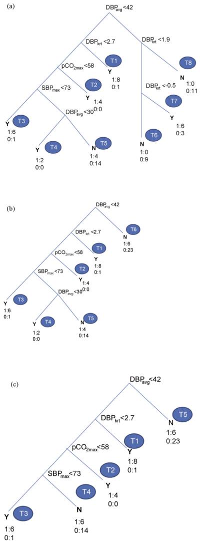
Decision tree with MLP selected features (a) full, (b) pruned (level 1) and (c) pruned (level 2).

At the root of DT is DBP_avg which represents the most significant one of the retained variables. In the next level is DBP_krt followed with pCO_2max and SBP_max in the order of importance. There are 8 terminal nodes (leaves) each with a class assigned (N: PVL = 0 or Y: PVL = 1) based on the majority of the members at the terminal node. In Fig. 2(a), the class membership is also shown at each leaf node corresponding to the training dataset for easy reference. For example, node T1 is classified as Y with 8 cases of 1 (PVL = 1) and 1 case of 0 (PVL = 0). The total number of decision rules is equal to the number of terminal nodes (leaves: T1-T8). The rules can be generated following the decision nodes from the root to each leaf through the corresponding branches. For example, the decision rule corresponding to the top most terminal node on the left (T1) can be obtained as follows:

$$\begin{array}{cc}\hfill \mathsf{I}f& {\mathsf{DBP}}_{\mathsf{avg}}<42\mathit{and}{\mathsf{DBP}}_{\mathsf{krt}}>2.7\mathit{then}\hfill \\ \hfill & \to \mathsf{Class}\mathsf{Y}(\mathsf{PVL}=1)(8∕9\mathsf{or}90\%)\hfill \end{array}$$

The set of decision rules for the full DTof Fig. 2(a) is given in Table 3(a). The above rule corresponds to the Rule #1 in Table 3(a) for terminal node T1. The class membership of node T1 is 8:PVL = 1 and 1:PVL = 0 with 90% as Y. Similarly, Rule #2 denotes the next leaf node (T2) on the left. Likewise the remaining rules of Table 3(a) can be obtained from the DT of Fig. 2(a). Rule #7 corresponds to leaf node (T7) on the right. This specifies a lower bound on DBP_avg (>42 mm Hg) and a bounded range for DBP_krt, i.e., -0.5 < DBP_krt < 1.9 for class Y (PVL = 1) with a membership of 67% (6 out of 9). The classification success for the training dataset was obtained collecting the proportion of correct classification of Y (corresponding to nodes with class Y in Table 3(a)) for SN, as follows: SN = (8 + 4 + 6 + 2 + 6)/30 = 87%. Similarly for SP and AC the performance indices were obtained as SP = (14 + 9 + 11)/39 = 87%, AC = (26 + 34)/69 = 87%. The generated DT was used to predict the PVL incidence for the test dataset. The corresponding test classification success SN, SP and AC were obtained as 87, 79 and 82%, respectively. These along with prediction results for DT using different number of features (4-7) selected in MLP and PNN are presented later in Table 5. The test prediction success of DTwith selected features using CI classifiers was reasonably acceptable (about 80%) considering the limitations of the dataset.

Table 3.

Decision rule sets for DT with MLP selected features (a) full, (b) pruned (level 1) and (c) pruned (level 2)

Rule #	If	and	and	and	and	then	Class	Membership
	DBPavg (mm Hg)	DBPkrt	pCO2max (mm Hg)	SBPmax (mm Hg)	DBPavg (mm Hg)		Y (PVL = 1)/N (PVL = 0)	Class/total	%
(a) Full
1	<42	>2.7					Y	8/9	90
2	<42	<2.7	>58				Y	4/4	100
3	<42	<2.7	<58	<73			Y	6/7	86
4	<42	<2.7	<58	<73	<30		Y	2/2	100
5	<42	<2.7	<58	<73	>30		N	14/18	78
6	>42	<-0.5					N	9/9	100
7	>42	<1.9					Y	6/9	67
		>-0.5
8	>42	>1.9					N	11/11	100
Rule #	If	and	and	and	and	then	Class	Membership
	DBPavg (mm Hg)	DBPkrt	pCO2max (mm Hg)	SBPmax (mm Hg)	DBPavg (mm Hg)		Y (PVL = 1)/N (PVL = 0)	Class/total	%
(b) Pruned (level 1)
1	<42	>2.7					Y	8/9	90
2	<42	<2.7	>58				Y	4/4	100
3	<42	<2.7	<58	<73			Y	6/7	86
4	<42	<2.7	<58	<73	<30		Y	2/2	100
5	<42	<2.7	<58	<73	>30		N	14/18	78
6	>42						N	23/29	79
Rule #	If	and	and	and	and	then	Class	Membership
	DBPavg (mm Hg)	DBPkrt	pCO2max (mm Hg)	SBPmax (mm Hg)	DBPavg (mm Hg)		Y (PVL = 1)/N (PVL = 0)	Class/total	%
(c) Pruned (level 2)
1	<42	>2.7					Y	8/9	90
2	<42	<2.7	>58				Y	4/4	100
3	<42	<2.7	<58	<73			Y	6/7	86
4	<42	<2.7	<58	>73			N	14/20	70
5	>42						N	23/29	79

Table 5.

Prediction results of DT using CI selected features

Classifier	Number of features	Training success (%)			Test success (%)
		SN	SP	AC	SN	SP	AC
MLP	4	77	92	86	27	58	44
	5	97	85	90	73	47	59
	6	90	80	84	80	74	77
	7	87	87	87	87	79	82
PNN	4	93	92	93	47	90	71
	5	100	82	90	73	68	71
	6	87	90	88	87	74	79
	7	90	90	90	73	68	71

3.3.2. Interpretation of decision rules

Rule 1 predicts PVL incidence if the DBP_avg is less than 42 mm Hg coupled with abrupt fluctuations in DBP (DBP_krt > 2.7). This simulates the situation of hypotension with rapid changes in DBP. In a previous work [32] on the same dataset with admission, maximum and minimum values of the postoperative monitoring hemodynamic variables, the case of hypotension was predicted. It is significant that in the present work, in addition to the threshold value on DBP, the distribution of DBP (DBP_krt) was identified as an additional indicator of PVL incidence. Similarly, Rule #2 predicts incidence of PVL if DBP_avg is below the threshold value (42 mm Hg) and change in DBP is moderate (DBP_krt < 2.7) but pCO_2max is above 58 mm Hg. This corresponds to combined hypotension and hypercarbia and is interesting to view in light of the prior work of Licht et al. [33].

In Licht et al. [33], MRI evidence of PVL was associated with low baseline values for cerebral blood flow as well as with diminished reactivity of cerebral blood flow to a hypercarbic gas mixture. It is interesting to note that some rules suggest lowest minimum or low admission pCO₂ may be important as risk factors for PVL, whereas Rule #2 above suggests thathypercarbia may be important. The retrospective nature of the study design, and the low sampling rate both may play a role in making explanation of variation in risk with variation in pCO₂ purely speculative. The levels of pCO₂ may have changed significantly inbetween the 4 h recording intervals. Although the design of this study prevents definitive ascertainment, the postoperative management style in use during the study period tended to value lower pCO₂ to decrease pulmonary vasoreactivity. Patients in the dataset with higher pCO₂ may have had issues with their ventilatory support leading to altered gas exchange and neurological susceptibility.

Similarly, Rule #3 corresponds to hypotension, both diastolic (DBP_avg < 42 mm Hg) and systolic (SBP_max < 73 mm Hg). This agrees with Rule #4 corresponding to the case of diastolic hypotension (DBP_avg < 30 mm Hg) even with SBP_max > 73 mm. Rule #5 predicts no PVL if SBP_max is above 73 mm Hg and the DBP_avg is within a range, i.e., 30 < DBP_avg < 42 mm Hg with moderate fluctuations in DBP (DBP_krt < 2.7). Rule #6 predicts no occurrence of PVL if DBP_avg is above 42 mm Hg and a flatter DBP (DBP_krt < -0.5). Rule #7 predicts incidence of PVL (6 out of 9) if DBP_avg > 42 mm Hg and bounded DBP variation, i.e., -0.5 < DBP_krt < 1.9. Rule #8 predicts no PVL if DBP_avg > 42 mm Hg and changes in DBP are moderate (DBP_krt > 1.9).

3.3.3. Decision tree pruning

The DTof Fig. 2(a) was pruned at level 1 to reduce the number of leaf nodes and the decision rules. The level 1 pruning combined all three terminal nodes on the right (T6-T8) into one (T6) and kept all other nodes on the left intact, Fig. 2(b). The leaf node on the right represented collectively the class N (PVL = 0) with a membership of 23/29 or 79% for DBP_avg > 42 mm Hg. The last 3 decision rules of Table 4(a) reduced to one rule (Rule #6) in Table 3(b). The training classification performance of the pruned DT (level 1) reduced with SN, SP and AC as 67, 95 and 83%, respectively. However, there was no change in the prediction performance for the test dataset (SN, SP, AC as 87, 79 and 82%, respectively). The DT of Fig. 2(b) was further pruned to the next level which combined terminal nodes T4 and T5 into one (T4), as in Fig. 2(c). The rule set of Table 3(b) reduced to 5 combining Rules #4 and #5 into one Rule #4 and with Rule #6 renumbered as #5 in Table 3(c). The prediction performance reduced slightly with SN, SP, AC as 60, 95, 80% in training and 80, 79, 79% in test, respectively. The classification success was reasonable even with the simplified (pruned) DT and the reduced set of decision rules. The pruning helped reduce the chance of overfitting the training data.

Table 4.

Decision rule sets for DT with PNN selected features (a) full, (b) pruned (level 1) and (c) pruned (level 2)

Rule #	If	and	and	and	and	then	Class	Membership
	DBPavg (mm Hg)	pCO2adm (mm Hg)	SBPavg (mm Hg)	pCO2min (mm Hg)	SBPmax (mm Hg)		Y (PVL = 1)/N (PVL = 0)	Class/total	%
(a) Full
1	<42	>31	<73	<28			N	3/4	75
2	<42	>31	<73	>28			Y	6/6	100
3	<42	>31	>73				N	7/7	100
4	<42	<31		>39			N	2/2	100
5	<42	<24		<39			N	2/3	67
6	<42	<31			<114		Y	16/17	94
		>24
7	<42	<31			>114		N	1/1	100
		>24
8	>42		<78				N	6/6	100
	<46
9	>46		<78				Y	5/8	63
10	>46		>78				N	14/15	93
Rule #	If	and	and	and	and	then	Class	Membership
	DBPavg (mm Hg)	pCO2adm (mm Hg)	SBPavg (mm Hg)	pCO2min (mm Hg)	SBPmax (mm Hg)		Y (PVL = 1)/N (PVL = 0)	Class/total	%
(b) Pruned (level 1)
1	<42	>31	<73	<28			N	3/4	75
2	<42	>31	<73	>28			Y	6/6	100
3	<42	>31	>73				N	7/7	100
4	<42	<31		>39			N	2/2	100
5	<42	<31		<39			Y	17/21	81
6	>42						N	23/29	79

Rule #	If	and	and	then	Class	Membership
	DBPavg (mm Hg)	pCO2adm (mm Hg)	SBPavg (mm Hg)		Y (PVL = 1)/N (PVL = 0)	Class/total	%
(c) Pruned (level 2)
1	<42	>31	<73		Y	7/10	70
2	<42	>31	>73		N	7/7	100
3	<42	<31			Y	17/23	74
4	>42				N	23/29	79

3.4. Results of decision tree algorithm with PNN selected features

The procedure of generating the DT was repeated using the training dataset with PNN selected 7 features (HR_adm, SBP_max, SBP_avg, DBP_avg, pCO_2adm, pCO_2min and pCO_2avg) leading to DTof Fig. 3(a). Here again, only 5 out 7 features were retained in the DT (DBP_avg, pCO_2adm, pCO_2min, SBP_avg and SBP_max) and others were eliminated due to their correlations with retained features. DT of Fig. 3(a) has 10 terminal nodes (T1-T10) with 10 decision rules as shown in Table 4(a). The classification success (SN, SP and AC) was 90% in training and 73, 68, 71% respectively in test. When the DTwas pruned to level 1, terminal nodes (T5-T7) were combined to one node (T5) and the right side nodes (T8-T10) collapsed to T6 leading to 6 decision rules of Table 4(b). The corresponding classification performance (SN and AC) reduced to 77%, 84% in training and improved to 87%, 77% in test with no change in SP. This confirms the effects of DT pruning on better generalization of test dataset with a moderate deterioration in the training success. When the DTof Fig. 3(b) was further pruned to level 2, leaf nodes T1, T2 collapsed into T1 and T4, T5 became T3 resulting in a much simpler DT of Fig. 3(c) with only 4 terminal nodes (T1-T4). The prediction performance (SN, SP and AC) changed to 80, 77 and 78% in training with no change in test (87, 68 and 77%). The corresponding rule set is given in Table 4(c). Rule #1 of the level 2 pruned DT predicts PVL corresponding to hypotension (DBP_avg < 42 mm Hg and SBP_avg < 73 mm Hg) even if pCO_2adm is above 31 mm Hg. Rule #2 predicts no PVL if SBP_avg is above 73 mm Hg even if DBP_avg is below 42 mm Hg. Rule #3 predicts PVL when DBP_avg is below 42 mm Hg and pCO_2adm is below 31 mm Hg. This condition represents diastolic hypotension combined with hypocarbia. The condition of hypotension agreed well with the results of previous section and of [32]. The association of hypocarbia with PVL has been reported earlier [34,35] and is a topic of interest in our centers as well as the subject of future analysis.

Figure 3.

Decision tree with PNN selected features (a) full, (b) pruned (level 1) and (c) pruned (level 2).

3.5. Decision tree prediction results

The selected features from the CI were used as inputs to the decision tree algorithm for classification. In each case, the training dataset was used to train the decision tree and the trained decision tree was tested using the test dataset. The classification success results are shown in Table 5 for different numbers of CI selected features (4-7). With the introduction of DT, the classification success in training reduced slightly compared to 100% for CI only. The classification performance improved with higher number of selected features and the training performance was reasonably good with 6 and 7 selected features. For DTwith MLP selected features (6 and 7), the ranges of SN, SP and AC were 87-90%, 80-87% and 84-87%, respectively in training. Corresponding test results were 80-87% (SN), 74-79% (SP) and 77-82% (AC). For DTwith PNN selected 6-7 features, the prediction success was 87-90% (SN), 90% (SP), 88-90% (AC) in training and 73-87% (SN), 68-74% (SP), 71-79% (AC) in test. There was not much difference in test performance between MLP and PNN, though the feature sets selected were slightly different.

3.6. Comparison of prediction performance

The prediction performance of CI was better than DT (of Part I) both in training (AC 100% vs. 91-96%) and test (74% vs. 62-65%). The performance of DT with CI selected features reduced slightly than CI only in training (AC 87-90% vs. 100%) but improved in test (AC 79-82% vs. 74%). For easy comparison, the best results of classification accuracy (AC) are shown for CI classifiers (test) and CI with DT (CIDT), both training and test, in Fig. 4. The better performance of the combined CI and DT based approach could be attributed to the inherent noise rejection capability of the feature selection process using CI and further refinement on the selected (more relevant) features using the information-gain algorithm of DT. On the other hand, DT algorithm tries to accommodate all the training cases in the induction of decision rules leading to a reasonable training success but with unsatisfactory test performance, especially in the presence of noise and uncertainties in the dataset. The introduction of DT with the CI selected features led to decision rule sets which are easy to interpret and would be expected to have better acceptability in clinical setting. When used with DT, the CI selected features gave better test performance than LR selected features (AC 79-82% vs.65%) of Part I. The improved performance of CI may be attributed to the greater generalization capability of CI than the inherent linear relationship of the independent variables (predictors) and the logarithm of odds ratio (OR) of the dependent variable (incidence of PVL) in LR. However, there is a need for more extensive dataset to investigate further the relative advantages of the CI, DT, LR and their combinations. This also needs to be compared with a direct information theoretical approach for optimal feature selection [36]. The use of other classifiers and data mining techniques like Kohonen self-organizing map (SOM) and support vector machines (SVM) needs to be considered in future studies.

Figure 4.

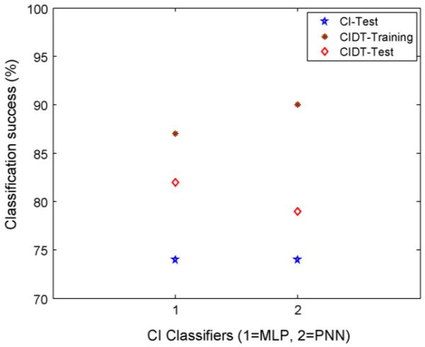
Comparison of classification success of CI classifiers with and without DT.

4. Conclusions

The paper presents results of investigations through CI techniques for prediction of PVL in neonates with CHD using postoperative hemodynamic and arterial blood gas data. The process involved statistical feature extraction, feature selection using CI techniques and generation of classification rules using DT algorithm. The CI based selection of prognostic features was further refined in DT algorithm resulting in a reduced set of decision rules that were quite easy to interpret. The combination of CI and DT gave much better test results than using these separately. The proposed combination also resulted in much better test performance than LR. The results show the advantages of using the proposed techniques of combined CI and DT for prediction of PVL, not only in terms of better prediction performance compared to LR but also with easily interpretable decision rules. The improved performance of the present approach may be attributed to the better generalization capability of the two-stage selection process of CI and DT. The availability of reduced set of easily tractable decision rule would be expected to have better acceptability of the present approach in the clinical setting.

The results confirmed the association of PVL incidence with hypotension, both diastolic (DBP_avg) and systolic (SBP_avg and SBP_max), consistent with an earlier study using the same original dataset. In addition to the average value, the temporal feature like kurtosis (DBP_krt) was also selected as a potential risk factor in one of the models. The present models also identified pCO₂ as a potential risk factor as in Part I. Future work is planned for validation of the proposed approach with a more extensive dataset and a direct information theoretic approach for optimal feature selection.

References

- [1].Kusiak A, Kern JA, Kernstine KH, Tseng BTL. Autonomous decision-making: a data mining approach. IEEE Trans Inform Tech Biomed. 2000;4:274–84. doi: 10.1109/4233.897059. [DOI] [PubMed] [Google Scholar]
- [2].Kononenko I. Machine learning for medical diagnosis: history, state of the art and perspective. Artif Intell Med. 2001;23:89–109. doi: 10.1016/s0933-3657(01)00077-x. [DOI] [PubMed] [Google Scholar]
- [3].Lisoba PSG. A review of evidence of health benefit from artificial neural networks in medical intervention. Neural Network. 2002;15:11–39. doi: 10.1016/s0893-6080(01)00111-3. [DOI] [PubMed] [Google Scholar]
- [4].Dounias G, Linkens D. Adaptive systems and hybrid computational intelligence in medicine. Artif Intell Med. 2004;32:151–5. doi: 10.1016/j.artmed.2004.07.005. [DOI] [PubMed] [Google Scholar]
- [5].Grobman WA, Stamilio DM. Methods of clinical prediction. Am J Obstet Gynecol. 2006;194:888–94. doi: 10.1016/j.ajog.2005.09.002. [DOI] [PubMed] [Google Scholar]
- [6].Tan KC, Yu Q, Heng CM, Lee TH. Evolutionary computing for knowledge discovery in medical diagnosis. Artif Intell Med. 2003;27:129–54. doi: 10.1016/s0933-3657(03)00002-2. [DOI] [PubMed] [Google Scholar]
- [7].Dreiseitl S, Ohno-Machado L. Logistic regression and artificial network classification models: a methodology review. J Biomed Inform. 2002;35:352–9. doi: 10.1016/s1532-0464(03)00034-0. [DOI] [PubMed] [Google Scholar]
- [8].Kitsantas P, Hollander M, Li L. Using classification trees to assess low birth weight outcomes. Artif Intell Med. 2006;38:275–89. doi: 10.1016/j.artmed.2006.03.008. [DOI] [PubMed] [Google Scholar]
- [9].Long WJ, Griffith JL, Selker HP, D’Agostino RB. A comparison of logistic regression to decision-tree induction in a medical domain. Comput Biomed Res. 1993;26:74–97. doi: 10.1006/cbmr.1993.1005. [DOI] [PubMed] [Google Scholar]
- [10].Perlich C, Provost F, Simonoff JS. Tree induction vs. logistic regression: a learning-curve analysis. J Mach Learn Res. 2003;4:211–55. [Google Scholar]
- [11].Green M, Björk J, Forberg J, Ekelund U, Edenbrandt L, Ohlsson M. Comparison between neural networks and multiple logistic regression to predict acute coronary syndrome in the emergency room. Artif Intell Med. 2006;38:305–18. doi: 10.1016/j.artmed.2006.07.006. [DOI] [PubMed] [Google Scholar]
- [12].Duh M-S, Walker AM, Pagano M, Kronlund K. Prediction and cross-validation of neural networks versus logistic regression: using hepatic disorder as an example. Am J Epidemiol. 1998;147:407–13. doi: 10.1093/oxfordjournals.aje.a009464. [DOI] [PubMed] [Google Scholar]
- [13].Song JH, Venkatesh SS, Conant EA, Arger PH, Sehgal CM. Comparative analysis of logistic regression and artificial neural network for computer-aided diagnosis of breast masses. Acad Radiol. 2005;12:487–95. doi: 10.1016/j.acra.2004.12.016. [DOI] [PubMed] [Google Scholar]
- [14].Erol FS, Usyal H, Erguin U, Barisci N, Serhathoglu S, Hardalac F. Prediction of minor head injured patients using logistic regression and MLP neural network. J Med Syst. 2005;29:205–15. doi: 10.1007/s10916-005-5181-x. [DOI] [PubMed] [Google Scholar]
- [15].Fabian J, Farbiarz J, Alvarez D, Martinez C. Comparison between logistic regression and neural networks to predict death in patients with suspected sepsis in emergency room. Crit Care. 2005;9:R150–6. doi: 10.1186/cc3054. [DOI] [PMC free article] [PubMed] [Google Scholar]
- [16].Nguyen T, Malley R, Inkelis SH, Kupppermann N. Comparison of prediction models for adverse outcome in pediatric meningococcal disease using artificial neural network and logistic regression analyses. J Clin Epidemiol. 2002;55:687–95. doi: 10.1016/s0895-4356(02)00394-3. [DOI] [PubMed] [Google Scholar]
- [17].Biesheuvel CJ, Siccama I, Grobbee DE, Moons KGM. Genetic programming outperformed multivariable logistic regression in diagnosing pulmonary embolism. J Clin Epidemiol. 2004;57:551–60. doi: 10.1016/j.jclinepi.2003.10.011. [DOI] [PubMed] [Google Scholar]
- [18].Delen D, Walker G, Kadam A. Predicting breast cancer survivability: a comparison of three data mining methods. Artif Intell Med. 2005;34:113–27. doi: 10.1016/j.artmed.2004.07.002. [DOI] [PubMed] [Google Scholar]
- [19].Phillips-Wren G, Sharkey P, Dy SM. Mining lung cancer patient data to assess healthcare resource utilization. Expert Syst Appl. 2008;35:1611–9. [Google Scholar]
- [20].Kurt I, Ture M, Kurum AT. Comparing performances of logistic regression, classification and regression tree, and neural networks for predicting coronary artery disease. Expert Syst Appl. 2008;34:366–74. [Google Scholar]
- [21].Samanta B, Nataraj C. Automated diagnosis of cardiac state in healthcare systems. Int J Serv Oper Inform. 2008;3:162–77. [Google Scholar]
- [22].Samanta B. Gear fault detection using artificial neural networks and support vector machines with genetic algorithms. Mech Syst Signal Process. 2004;18:625–44. [Google Scholar]
- [23].Samanta B. Artificial neural networks and genetic algorithms for gear fault detection. Mech Syst Signal Process. 2004;18:1273–82. [Google Scholar]
- [24].Samanta B, Al-Balushi KR, Al-Araimi SA. Artificial neural networks and genetic algorithm for bearing fault detection. J Soft Comput. 2005;10:264–71. [Google Scholar]
- [25].Samanta B, Nataraj C. Prognostics of machine condition using soft computing. Robot Comput Integrated Manuf. 2008;24:816–23. [Google Scholar]
- [26].Samanta B, Nataraj C. Surface roughness prediction in machining using computational intelligence. Int J Manuf Res. 2008;3:379–92. [Google Scholar]
- [27].Samanta B, Erevelles W, Omurtag Y. Prediction of workpiece surface roughness using soft computing. Proc IME B J Eng Manufact. 2008;222:1221–32. [Google Scholar]
- [28].Samanta B, Bird GL, Kuijpers M, Zimmerman RA, Jarvik GP, Wernovsky G, et al. Prediction of periventricular leukomalacia. Part I: Selection of features using logistic regression and decision tree algorithms. Artif Intell Med. 2008 doi: 10.1016/j.artmed.2008.12.005. doi:10.1016/j.artmed.2008.12.005. [DOI] [PMC free article] [PubMed] [Google Scholar]
- [29].Haykin S. Neural networks: a comprehensive foundation. 2nd ed. Prentice-Hall; New Jersey, USA: 1999. [Google Scholar]
- [30].Wasserman PD. Advanced methods in neural computing. Van Nostrand Reinhold; New York, USA: 1995. pp. 35–55. [Google Scholar]
- [31].Michalewicz Z. Genetic algorithms + data structures = evolution programs. Springer-Verlag; New York, USA: 1999. [Google Scholar]
- [32].Galli KK, Zimmerman RA, Jarvik GP, Wernovsky G, Kuijpers M, Clancy RR, et al. Periventricular leukomalacia is common after cardiac surgery. J Thorac Cardiovasc Surg. 2004;127:692–702. doi: 10.1016/j.jtcvs.2003.09.053. [DOI] [PubMed] [Google Scholar]
- [33].Licht DJ, Wang J, Silvestre DW, Nicolson SC, Montenegro LM, Wernovsky G, et al. Preoperative cerebral blood flow is diminished in neonates with severe congenital heart defects. J Thorac Cardiovasc Surg. 2004;128:841–9. doi: 10.1016/j.jtcvs.2004.07.022. [DOI] [PubMed] [Google Scholar]
- [34].Okumura A, Hayakawa F, Kato T, Itomi K, Maruyama K, Ishihara N, et al. Hypocarbia in preterm infants with Periventricular leukomalacia: the relation between hypocarbia and mechanical ventilation. Pediatrics. 2001;107:469–75. doi: 10.1542/peds.107.3.469. [DOI] [PubMed] [Google Scholar]
- [35].Shankaran S, Langer JC, Kazzi SN, Laptook AR, Walsh M. Cumulative index of exposure to hypocarbia and hyperoxia as risk factors for periventricular leukomalacia in low birth weight infants. Pediatrics. 2006;118:1654–9. doi: 10.1542/peds.2005-2463. [DOI] [PubMed] [Google Scholar]
- [36].Koller D, Sahami M. Toward optimal feature selection; Proceedings of 13th international conference on machine learning (ICML); 1996.pp. 284–92. [Google Scholar]