

Abstract
Mathematical models of radiation carcinogenesis are important for understanding mechanisms and for interpreting or extrapolating risk. There are two classes of such models: (1) long-term formalisms that track pre-malignant cell numbers throughout an entire lifetime but treat initial radiation dose–response simplistically and (2) short-term formalisms that provide a detailed initial dose–response even for complicated radiation protocols, but address its modulation during the subsequent cancer latency period only indirectly. We argue that integrating short- and long-term models is needed. As an example of this novel approach, we integrate a stochastic short-term initiation/inactivation/repopulation model with a deterministic two-stage long-term model. Within this new formalism, the following assumptions are implemented: radiation initiates, promotes, or kills pre-malignant cells; a pre-malignant cell generates a clone, which, if it survives, quickly reaches a size limitation; the clone subsequently grows more slowly and can eventually generate a malignant cell; the carcinogenic potential of pre-malignant cells decreases with age.
Introduction
Short- and long-term biologically based models
Biologically motivated mathematical modeling of background and ionizing radiation-induced carcinogenesis has a history spanning more than 50 years (Nordling 1953). Many of the models can be characterized as short-term, in that they focus on processes occurring during and shortly after irradiation (Hahnfeldt and Hlatky 1998; Radivoyevitch et al. 2001; Mebust et al. 2002; Schollnberger et al. 2002; Sachs and Brenner 2005; Hofmann et al. 2006; Shuryak et al. 2006; Little 2007; Sachs et al. 2007; Schneider and Walsh 2008). The main advantage of such models is that they provide a detailed initial dose–response relation for short-term endpoints, which are used as surrogates for carcinogenesis. The main disadvantage is that the possibly substantial modulations of the magnitude and shape of this initial dose–response during the lengthy period (multiple years-decades) between irradiation and manifestation of typical solid tumors are not considered mechanistically.
In contrast, another class of biologically motivated models can be characterized as long-term, in the sense that they track carcinogenesis rates throughout the entire life span, e.g., the Armitage-Doll model (Armitage and Doll 1954; Armitage 1985), the Moolgavkar-Venzon-Knudson two-stage clonal expansion (TSCE) model (Moolgavkar 1978, 1980; Moolgavkar and Knudson 1981), the two-stage logistic model (Sachs et al. 2005), and many others (Yakovlev and Polig 1996; Pierce and Mendelsohn 1999; Wheldon et al. 2000; Little and Wright 2003; Pierce and Vaeth 2003; Ritter et al. 2003; Little and Li 2007). The main advantage of long-term models is the more detailed treatment of slow carcinogenesis processes, including the modulation of the radiation dose–response during the long latency period. The main disadvantage is that the initial dose–response is typically treated in a non-mechanistic, phenomenological manner.
The need for a new approach: integration of long- and short-term models
The lack of detailed treatment of radiation-specific effects typically limits risk predictions from long-term models to exposure conditions where a simple dose–response relationship holds. Exposures where this relationship is more complex, such as high fractionated radiotherapeutic doses that can lead to treatment-induced cancers in nearby organs (Travis et al. 1996, 1997, 2002, 2003; van Leeuwen et al. 2003; Travis et al. 2005) are difficult to describe with current long-term models. Conversely, the more detailed dose–responses produced by sophisticated short-term models can be scaled to cancer risks only by considering the effects of factors such as background risks, age at exposure, and time since exposure, which are not explicitly taken into account by the short-term formalisms. A new, unified approach of integrating short- and long-term techniques is needed, where a detailed initial dose–response for pre-malignant cell numbers is produced over a wide range of doses, and changes to the shape of this dose–response during the latency period before the development of cancer are also analyzed in detail. A schematic representation of model unification is provided in Fig. 1.
Fig. 1.

A general scheme of short- and long-term processes governing the total number of pre-malignant cells. Details are discussed throughout the main text. As the individual ages, the number of viable pre-malignant cells grows, but the curve may turn over and decrease at very old age (blue line in the main graph). This pattern parallels background cancer incidence, since cancer risk is assumed to be proportional to the number of pre-malignant cells (discussed in the text). Radiation exposure (e.g., radiotherapy for an existing cancer) initially causes the number of pre-malignant cells to decrease due to cell killing (red line). After exposure stops, the irradiated tissues recover, allowing pre-malignant cells to repopulate and reach a number higher than was present before irradiation, i.e., a net excess radiogenic cancer risk is produced. Fluctuations in the number of pre-malignant cells throughout the irradiation and recovery periods (i.e., the short-term processes) are shown in the inset graph
Motivations for the specific unification used here
Here, we provide a specific example of integrating short- and long-term radiation carcinogenesis models. In that a variety of short- and long-term models have been proposed, our approach should be considered as illustrative, intended to investigate the practicality of integrating the two model types. The goal was to produce a novel formalism, which can describe typical patterns of background and radiogenic carcinogenesis with the smallest possible number of adjustable parameters. This goal required multiple simplifying assumptions about the complex multi-step carcinogenesis process. We suggest that for the purposes of generating a preliminary integrated model, the consequent reduction in biological realism is compensated by the reduction in model complexity and number of parameters. More complicated examples of unifying long- and short-term models are certainly possible, e.g., models analyzing multiple pre-malignant cell stages, analyzing genomic instability, and/or analyzing stochastic effects at both time scales, rather than just at short-time scales as we shall do.
Short-term model
The short-term part of our model (Fig. 1a) is the more mathematically intensive part of the integrated formalism. It is based on existing initiation, inactivation and repopulation (iir) models originally designed for analyzing second cancers induced by radiotherapy (Lindsay et al. 2001; Sachs and Brenner 2005; Shuryak et al. 2006; Little 2007; Sachs et al. 2007). This short-term part analyzes normal and pre-malignant stem cells during complex radiation exposure regimens and during the following weeks of tissue recovery. It tracks individual pre-malignant cell clones rather than just the total number of pre-malignant cells. The probability that a pre-malignant clone becomes extinct during radiotherapy can be substantial, so a fully stochastic formalism is used for the population dynamics of pre-malignant cells.
Long-term model
The long-term part of our model (Fig. 1b) approximates carcinogenesis by a process where normal target (e.g., stem) cells can be initiated by spontaneous or radiation-induced mutations to become pre-malignant cells, which can clonally expand and perhaps produce by mutation a fully malignant cell, which then gives rise to cancer after some lag period. The basic assumptions are somewhat similar to those of several long-term models cited above, including the TSCE model. Specifically, our long-term formalism uses the following main assumptions:
Normal and pre-malignant stem cells are located in specific tissue niches (Slack 2000; Borthwick et al. 2001; Potten and Booth 2002; Bennett et al. 2003; Fuchs et al. 2004; Ghazizadeh and Taichman 2005; Li and Xie 2005). We here have in mind a general concept of a niche, including, e.g., a clone whose further growth is prevented or slowed by any kind of micro-environmental constraints. The number of niches per organ, and the number of normal or pre-malignant stem cells per niche, is homeostatically regulated (Fuchs et al. 2004; Li and Xie 2005). We allow for the possibility that pre-malignant stem cells are regulated somewhat less stringently than their normal counterparts, so that a niche filled with pre-malignant cells can contain more such cells on average than a niche filled with normal cells.
An initiated stem cell either dies out, or grows into a pre-malignant clone, which quickly (e.g., within a year, Campbell et al. 1996) fills the entire stem cell niche in which it originated, i.e., “initiates” the whole niche. To expand beyond the first niche, the pre-malignant clone needs to invade an adjacent niche; alternatively, the niche containing the clone can divide into two daughter niches, e.g., colon crypt fission (Greaves et al. 2006; Johnston et al. 2007; Edwards and Chapman 2007). These processes require years or decades, and may involve acquisition of new mutations (Spencer et al. 2006).
Pre-malignant cells in all niches are assumed to gradually lose their carcinogenic potential with age, so that at old age they have a progressively smaller probability of being transformed to malignant cells. This assumption is suggested by a decrease in incidence of most cancers at very old age, e.g., >80 years in humans [Surveillance Epidemiology and End Results (SEER) database, http://seer.cancer.gov] and >800 days in mice (Pompei et al. 2001). The likely mechanism is senescence of stem cells and/or deterioration of stem cell function, or niche function, with age (Brunet and Rando 2007; Carlson and Conboy 2007; Sharpless and DePinho 2007).
To reduce the number of model parameters, clonal expansion of pre-malignant stem cell niches is treated deterministically, using a net proliferation rate. In other words, it is estimated by a deterministic “exponential model”, instead of the stochastic TSCE model. Given realistic parameter values, the deterministic and stochastic versions of the two-stage model are numerically very similar from birth until old age (Heidenreich and Hoogenveen 2001). In our analyses, by the time irradiation is over and cell repopulation in the exposed organ has occurred, surviving pre-malignant clones have grown to substantial sizes, making extinction very unlikely. This reduces the need for stochastic treatment of clone dynamics during the decades following radiation exposure. At old age, the deterministic approximation predicts an increasing hazard, whereas the stochastic TSCE model predicts a plateau. Considering the evidence cited above about a decrease in cancer incidence at old age, neither behavior is fully realistic. We here instead model the downturn in incidence at old age explicitly, according to the assumption above.
Unification of short- and long-term models
The integration of long- and short-term models will have two features typical of multi-timescale modeling (Engquist and Runborg 2005): (1) information is passed in both directions between the two components; and (2) a formally infinite time interval in the short-term model represents a short time interval, here typically several months, in the long-term model (Fig. 1).
The deterministic long-term equations provide the mean number of niches filled with pre-malignant stem cells and the mean number of pre-malignant cells per niche just before irradiation. The stochastic short-term equations then provide the number of these niches that are eradicated by radiation as well as the number of pre-malignant clones that are induced by, and survive, the radiation exposure. Each of these clones is assumed to be independent (i.e., located in a different part of the organ), and to be capable of quickly filling a niche with pre-malignant cells. Therefore, the total number of pre-malignant niches soon after irradiation can be calculated by the stochastic short-term model. The mean of this number is the initial condition for the deterministic long-term equations, which are applied from this point onwards until old age (Fig. 1). Cancer incidence is assumed to be proportional to the total number of pre-malignant cells in all niches, shifted by a lag time. A mathematical description of the model is provided below.
Materials and methods
The mathematical techniques for implementing the assumptions for our specific example of integrating long- and short-term modeling are discussed next. A schematic representation of the concepts is provided in Fig. 2. The notation and interpretations for model parameters are listed in Table 1. Data on both background and radiation-induced cancers are used to estimate the parameters.
Fig. 2.

Schematic representation of proposed pre-malignant cell kinetics. Each square represents a tissue niche. Cyan color normal cells; other colors pre-malignant cells—each color indicates a different clone. Black arrows invasion of an adjacent niche. The order of panels denotes a hypothetical time sequence: a only niches filled with normal cells are present at a young age. b Some niches filled with pre-malignant cells are spontaneously initiated (red and blue). c–e The pre-malignant clones expand over time by taking over adjacent niches. f Radiation exposure (lightning symbols) perturbs the system: some normal and pre-malignant cells are inactivated (niches become smaller), and some niches are completely inactivated (shown by gaps). Some new pre-malignant clones are initiated (green and brown). g After exposure, all niches filled with pre-malignant cells (red, blue, green, brown) expand in cell number (undergo promotion, shown by an increase in the size of the squares). Possible promotion of normal niches is neglected. Surviving normal and pre-malignant niches replace the niches inactivated by radiation (shown by disappearance of the gaps). h Over many years/decades after irradiation, roughly normal tissue architecture is restored. The promoting effect may disappear, as all niches return to the default size. Meanwhile, replication of existing pre-malignant niches continues (shown by arrows), and some new clones appear by spontaneous initiation (shown by the black square). i Subsequent mutations in one of the pre-malignant clones produce the first fully malignant cell, which grows into a malignant tumor (gray mass)
Table 1.
Summary of model parameters
| Parameter | Units | Interpretation |
|---|---|---|
| a | time−2 | Spontaneous stem cell initiation and transformation |
| b | time−1 | Pre-malignant niche replication |
| c | time−2 | Age-dependent pre-malignant cell senescence |
| δ | time−1 | Homeostatic regulation of pre-malignant cell number per niche |
| Z | cells/niche | Carrying capacity for pre-malignant cells per niche |
| X | time/dose | Radiation-induced initiation |
| Y | dose−1 | Radiation-induced promotion |
| α, β | dose−1, dose−2 | Stem cell inactivation by radiation |
| λ | time−1 | Maximum net stem cell proliferation (repopulation) rate |
| L | time | Lag period between the first malignant cell and cancer |
Long-term model for background cancers
The long-term model was intended mainly to place the results of the stochastic short-term calculations in an appropriate context, enabling estimation of the effects of age at exposure and time since exposure on predicted cancer risk. Simplicity and parsimony were emphasized. The long-term model in the absence of radiation consists just of a few rather simple deterministic equations, as follows.
Each pre-malignant stem cell in any niche has a certain small probability per unit time (q units = cells−1 × time−1) of transforming into a fully malignant cell, and, after a fixed lag time (L), into clinical cancer. These are common assumptions made in many long-term carcinogenesis models, e.g., in the TSCE model. The average number of new fully malignant cells per unit time (A units = time−1) is the product of q and three other variables: the number of stem cell niches filled with pre-malignant cells (M units = niches), the average number of pre-malignant stem cells per niche (ρ units = cells × niche−1), and the probability that the pre-malignant cells remain non-senescent and capable of producing cancer (P). The number of pre-malignant stem cells per niche (ρ) is assumed to be homeostatically regulated (in a qualitatively similar manner to the regulation of normal stem cells), so that it always tends towards a constant number—a carrying capacity Z (units = cells × niche−1). For convenience, the number of pre-malignant stem cells per niche can be redefined as a dimensionless normalized fraction C = ρ/Z. The proportionality constant qZ can be removed from the expression for A by defining N = qZM (units = time−1), where N is proportional to the number of pre-malignant niches. Consequently, A can be written in the following simplified form:
 |
1 |
Equation (1) is an approximation for the incidence hazard function: it gives the mean expected number of new malignant cells (i.e., eventual cancers) per individual per year, whereas the hazard (H) given in (2) is the yearly probability that a malignant cell occurs in a previously healthy individual at age t:
 |
2 |
The functions A and H are numerically very similar for realistic parameter values; they diverge substantially only if cancer incidence is high. We use the exact hazard H for data fitting in the companion paper, but use the simpler expression for A in the equations below, keeping in mind its interpretation and limitations.
The function N is described by the following differential equation (3), where t is patient age, the constant a (units = time−2) is proportional to the spontaneous stem cell initiation rate, and the constant b (units = time−1) is the pre-malignant niche replication rate:
 |
3 |
Equation (3) can be adjusted to accommodate an assumption that more than one mutation is needed to initiate a stem cell by replacing the constant a with the composite term at κ−1, where κ is the necessary number of mutations. However, doing so does not substantially improve the fit of the model to the data sets analyzed, and so was not used as the default because it introduces an extra adjustable parameter κ. The results for fitting multi-stage extensions of our model (i.e., where κ > 1) to SEER data for female breast and male lung cancers are shown in Fig. 3.
Fig. 3.

Fits of the long-term part of our model to spontaneous incidence data for female breast and male lung cancers from SEER (the data for young ages were excluded because cancer incidence in these age groups is likely to be dominated by genetic predisposition). Error bars represent 95% confidence intervals. The different curves represent our default two-stage formalism and its multi-stage extensions described in the main text. These extended versions of the formalism do not alter the fit substantially
The function C is regulated by the following logistic differential equation, where δ (units = time−1) is a rate constant representing the strength of homeostatic control of the number of pre-malignant cells per niche:
 |
4 |
For background carcinogenesis the solution C = 1 is used.
The probability that the pre-malignant cells remain non-senescent and capable of producing cancer (P) is described by a Gaussian function with an adjustable parameter c (units = time−2), which cannot become negative even as age approaches infinity, contrary to the expression used by Pompei et al. (2001) and Pompei and Wilson (2002):
 |
5 |
For convenience later, when radiation-induced excess relative risk (ERR) will be calculated, it is useful to express patient age (t) as the sum of age at exposure (T x) and time since exposure (T y). The background cancer risk function without radiation (A bac(T x, T y)) follows from (1) and (3–5), assuming that no pre-malignant cells are present at birth (i.e., that N(0) = 0):
 |
6 |
Here, the duration of radiation exposure is ignored, because it is considered to be short compared with the multi-year time scale of the long-term carcinogenesis processes.
Effects of radiation
Short-term processes
The exposure scenario analyzed here is radiotherapy for an existing malignancy, where there are K daily dose-fractions, all of equal size d in some nearby organ, with treatment gaps during the weekends. Straightforward generalizations to variable doses per fraction, to other temporal patterns, and/or to cases where one must consider dose-volume histograms are omitted for brevity. A single acute dose exposure is a simple special case, where the number of fractions is K = 1.
The short-term part of the model considers initiation, inactivation, and repopulation (iir) of normal and pre-malignant stem cells during the radiation regimen and a recovery period of about a month (Fig. 1). Niche takeover by pre-malignant cells that survive the irradiation and modulation of niche size by radiogenic promotion (discussed below) are here also considered short-term processes. They are assumed to be essentially completed by a few months following exposure, before the long-term processes of spontaneous initiation and niche replication, which operate on the time scale of multiple years, start to have an appreciable effect (Fig. 1).
Normal stem cells are treated deterministically because their number per organ is assumed to be large. In contrast, the number of pre-malignant stem cells per clone is much smaller, and extinction of some pre-malignant clones is a real possibility. Consequently, a stochastic approach described below is used to estimate the average number of live pre-malignant niches when post-irradiation long-term processes begin.
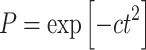
For simplicity, both normal and pre-malignant stem cells are assumed to be equally radiosensitive. The cell surviving fraction (S) is described by the standard linear-quadratic (LQ) function with parameters α and β for dose-fractions of size d:
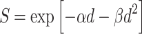 |
7 |
The normal stem cell number (n) in the entire organ just before the kth dose-fraction is denoted by n −(k), and the number just after the kth dose-fraction by n +(k). The reduction in n due to initiation of a few normal stem cells is neglected. Inactivation is calculated as follows:
 |
8 |
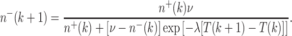
Repopulation of normal stem cells during radiotherapy is assumed to be regulated by homeostatic mechanisms—if some stem cells are killed by radiation, surviving stem cells are induced to proliferate (Dörr and Kummermehr 1990; Pabst et al. 2004) with the goal of restoring the total number of normal stem cells in the organ (n) to the number present before irradiation (ν). It should be noted that ν is conceptually and numerically distinct from the carrying capacity Z introduced above for pre-malignant stem cells per pre-malignant niche. The homeostatic regulation of cell proliferation during the time gaps between dose-fractions and after the last fraction is described by the Logistic differential equation, where λ (with units = time−1) is the maximum net proliferation rate:
 |
9 |
Equations (7–9) allow the calculation of the normal stem cell number n(t) in the entire organ at all relevant times t throughout the radiation exposure and recovery periods. Explicit results for n(t) are provided in the Appendix.
We assume that the long-term growth advantage of pre-malignant cells manifests itself only on the scale of years and decades, and is negligible on the much shorter time scale of a few weeks of radiotherapy. Consequently, the maximum net proliferation rates for normal and pre-malignant stem cells are assumed to be equal, described by the parameter λ.
As discussed above, radiation initiates some normal stem cells, making them pre-malignant. The number of cells initiated in the kth dose-fraction is assumed to be Poisson distributed, with average aXI(k), where X is an adjustable parameter (units = time × dose−1) and the function I(k) (units = dose) is given by:
 |
10 |
Our assumptions allow the birth, death, and initiation rates for normal stem cells calculated deterministically by (7–10) to be used as parameters for a stochastic formalism for pre-malignant cell clones. Each such clone is initiated as a single cell in some random niche by the kth dose-fraction, and can fluctuate in cell number during subsequent radiotherapy due to the opposing effects of inactivation and repopulation. We count the number of clones that contain at least one viable cell when radiotherapy ends, because only these surviving clones are capable of eventually taking over their niches. Their number is determined by the probability F(k) that a live stem cell initiated by the kth dose-fraction produces a clonal lineage, which survives all subsequent dose-fractions. Using analytic results on stochastic birth–death processes with variable rates (Tan 2002; Hanin 2004) the Appendix derives an equation, (22), for F(k), which is repeated here:
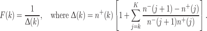 |
Here, F(0) is the probability that a pre-malignant cell that was present before irradiation began produces a lineage which survives all dose-fractions.
Using the facts that a random thinning of a Poisson distribution is Poisson and the sum of independent Poisson distributions is Poisson, one can show that the total number of surviving pre-malignant clones at the end of the short-term period is Poisson distributed. The above arguments give the mean value as N
init = aXISf(D), where D is the total radiation dose (i.e., the sum of all doses per fraction, dK) and ISf(D) (units = dose) represents a net outcome of initiation, inactivation, and cell repopulation during exposure,  The probability that a pre-malignant niche that was present before exposure is not inactivated by radiation (i.e., that at least one pre-malignant stem cell in the niche survives) is given by:
 |
11 |
Unifying short- and long-term processes
The above short-term processes are regarded as effectively instantaneous relative to the long-term ones. The stochastic results for the short-term exposure period, in the form of the functions ISf(D) and Sf(Z, D), are inserted into the deterministic equations for long-term carcinogenesis processes. On the long-term time scale, niches already pre-malignant at the end of irradiation and recovery then increase in number by replication; we will refer to all the resulting niches as “old” niches. Other, “new” niches are formed by spontaneous initiation after the end of the exposure period. The contributions of niches in these two categories to the cancer risk are called N rad E(T x, T y) and N rad N(T x, T y), respectively. At a given time (T y) after irradiation they are given by the following solutions for (3):
 |
12 |
Radiation is commonly assumed to promote hyper-proliferation of pre-malignant cells (Heidenreich et al. 2007). Here, we interpret this effect as an increase in the number of pre-malignant stem cells per surviving niche above the niche carrying capacity Z, i.e., C becomes >1. For simplicity, the initial excess of C is assumed to be linearly dependent on radiation dose with the coefficient Y (units = dose−1). Promotion may be eventually reversed, because the number of pre-malignant cells per pre-malignant niche may gradually return to pre-irradiation carrying capacity Z. This process may occur concurrently with extinction of some radiation-induced niches (Zhang et al. 2001; Ullrich 1986). Since only the product of the number of niches and the number of cells per niche is relevant for cancer risk (1), extinction of some niches and/or shrinkage of niche size do not need to be modeled separately. The net effect—i.e., a gradual reversal of promotion—can be modeled using only one adjustable parameter (δ), as done here. According to these assumptions, at any given time (T y) after exposure to radiation the average normalized number of pre-malignant cells per surviving niche (C rad(T x, T y)) can be calculated by solving (4):
 |
13 |
Calculation of absolute and relative cancer risks
The approximation for the absolute cancer risk after radiation (A rad(T x, T y)) can now be calculated at any age at exposure and time since exposure by using the equations above:
 |
14 |
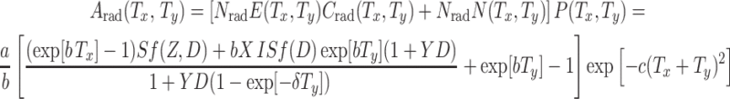
The excess relative cancer risk (ERR) follows from (6) and (14): ERR = [A rad(T x, T y)/A bac(T x, T y)] − 1. By substitution and simplification, a more explicit expression for the ERR can be obtained:
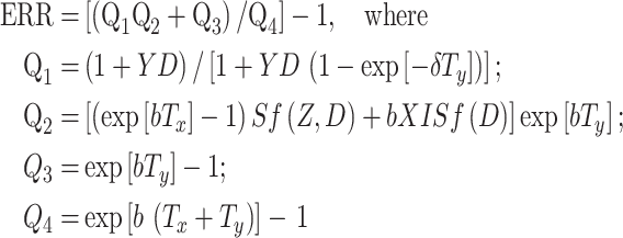 |
15 |
Note that the senescence parameter (c) cancels out of this ERR expression; due to the way we have defined our radiation initiation parameter (X), the spontaneous initiation parameter (a) also cancels out. The term Q 1 can be interpreted as the normalized size of old pre-malignant stem cell niches. Q 2 is proportional to the number of such niches. Q 3 is proportional to the number of new pre-malignant niches, and Q 4 is proportional to the total number of pre-malignant niches under background conditions.
Results
To display the properties of the model, we produced Figs. 4–7 using generic parameter values guided by the best-fit values for specific cancer sites found in the accompanying paper (Shuryak et al. 2009).
Fig. 4.

The typical shape for age dependence of background incidence for a specific type of adult-onset solid cancer is reasonably reproduced by our model. The curve was generated using the following parameter values: a = 1.0 × 10⁻⁸ y−2, b = 0.25 y−1, c = 1.75 × 10⁻³ y−2, L = 10 y
Fig. 7.

Modulation of promotion-driven excess relative cancer risk (ERR) over time after exposure: a low doses (either acute or fractionated produce similar results, since cell inactivation is negligible), b high fractionated doses (fractions are given once daily, with gaps on weekends). It is seen that, contrary to a proportional hazards assumption, not only the amplitude but also the shape of the dose–response curve is altered by long-term processes. The parameters were the same as in previous figures
Figure 4 shows an example of a model-generated age-dependent background incidence curve for an adult-onset solid cancer, using the four relevant parameters a, b, c, and L. The shape of this curve agrees well with the data for many cancers (e.g., SEER database, http://seer.cancer.gov), including the downturn in incidence at old age, which is not described as well by standard models.
Figure 5 shows a typical radiation dose–response, which is determined by the balance of cell initiation, inactivation (killing), and repopulation. Fractionation of the dose increases cancer ERR because repopulation of both normal and pre-malignant cells during the inter-fraction intervals compensates for much of the cell killing.
Fig. 5.

The effect of dose-fractionation on predicted excess relative cancer risk (ERR): as the same total radiation dose is split into fractions (one fraction per day, with gaps on weekends), thereby protracting it over a longer time, cancer risk predicted by the model increases. This occurs because cell repopulation during prolonged exposure partially compensates for cell killing by radiation. The doses refer to a given organ, such as the lungs or female breast, and not to whole body exposures. The following parameter values were used: b = 0.25 y−1, X = 10.0 y × Gy−1, Y = 0.5 Gy−1, δ = 0.01 y−1, Z = 10.0 cells/niche, α = 0.3 Gy−1, β = 0.0 Gy−2, λ = 0.35 day−1, T x = 30 y, T y = 0.0 y, and L = 10 y
Figures 6 and 7 show the effects of age at exposure and time since exposure. The components of cancer ERR produced by radiation-induced initiation and radiation-induced promotion exhibit very different dependences on age at exposure. Radiation is assumed to initiate the same number of cells per unit dose independent of age, whereas the background number of pre-malignant cells, which is essentially the denominator of ERR, grows with age. Consequently, the initiation-driven component of ERR decreases with age at exposure. This process dominates the ERR for ages <20 years in Fig. 6. In contrast, promotion is assumed to be a multiplicative amplification of the background number of pre-malignant cells per niche. Consequently, the promotion-driven component of ERR is approximately constant over most ages at exposure. This process dominates the ERR for older ages in Fig. 6.
Fig. 6.

Combined effects of age at exposure and time after exposure on radiation-induced excess relative cancer risk (ERR). The ERR is calculated at age 70, which is intended to approximate lifetime risk. As discussed in the text, only age at exposure matters if parameter δ = 0, but if δ > 0, time after exposure affects the ERR as well. The parameter values were the same as in Fig. 5, except for T x and T y, and a reference radiation dose of 1 Gy
Promotion-driven ERR can also be modulated by time after exposure. This occurs due to the assumption that the number of pre-malignant cells per niche is homeostatically regulated (by parameter δ), so that radiation-induced hyper-proliferation of cells within their niches can be reversed, as pre-irradiation cell birth/death rates, and hence niche sizes, are restored. If δ > 0, ERR due to promotion will decrease over time following exposure. This effect is seen in Figs. 6, 7: If the risk is measured at some constant age (e.g., 70 years), which is a sum of age at exposure and time since exposure, a decrease in ERR with time since exposure due to a δ > 0 will appear as an increase in the ERR with age at exposure (Fig. 6). A decrease in promotion-driven ERR with time since exposure also can have a conceptually important effect on the dose–response—at longer times after exposure, not only the magnitude, but also the shape, of the dose–response can change (Fig. 7).
Discussion
The formalism presented here is the first comprehensive attempt to unify short- and long-term modeling approaches. The short-term part of the model belongs to the previously discussed iir category. It tracks the numbers of pre-malignant cells throughout irradiation stochastically. The long-term part of the model builds on the concepts developed in previous two-stage formalisms by adding an analysis of some aspects of tissue architecture (i.e., stem cell niches/compartments) and aging of pre-malignant stem cells. The particular short and long-term models that we have chosen to use are not crucial—the real issue is the integration. Certainly other long-term models could perfectly well be integrated into this short-/long-term framework—and we hope they will be.
The unified formalism has a number of advantages. The short-term part can generate reasonable predictions even at high doses, such as those in cancer radiotherapy. The long-term part analyzes the entire lifetime of the individual, putting the short-term predictions in an appropriate context by estimating the effects of age at exposure and time since exposure. The combined approach therefore allows the dose–response for the number of pre-malignant cells to be examined at any time point, from the start of irradiation until development of cancer years to decades later, which is not possible using either short- or long-term models alone.
Our model can be used for estimating risks of second malignancies induced by radiotherapy. This issue is growing in importance (Brenner et al. 2000; Ron 2006) as patients are treated earlier in life and the number of cancer survivors increases (Editorial 2004); the lifetime risk of radiation-induced second cancers is not negligible (Brenner et al. 2007). Direct measurement of second cancer incidence requires decades of follow-up because the latency period for radiogenic solid tumors is long (Tokunaga et al. 1979; Brenner et al. 2000; Ivanov et al. 2004, 2009). Meanwhile, radiotherapy protocols are rapidly changing. Our model, calibrated using data from older protocols, can produce risk predictions for any modern or prospective radiotherapeutic protocol. This application of the model is discussed in the accompanying paper (Shuryak et al. 2009).
Acknowledgments
Research supported by National Cancer Institute grant 5T32-CA009529 (IS), Department Of Energy DE-FG02-03ER63668 and National Institutes of Health CA78496 (PH), National Aeronautics and Space Administration 03-OBPR-07-0059-0065(LH), National Aeronautics and Space Administration NSCOR NNJ04HJ12G/NNJ06HA28G (RKS), National Institutes of Health grants P41 EB002033-09 and P01 CA-49062 (DJB).
Open Access
This article is distributed under the terms of the Creative Commons Attribution Noncommercial License which permits any noncommercial use, distribution, and reproduction in any medium, provided the original author(s) and source are credited.
Appendix
This appendix gives some details on the equations for the short-term calculation and on their derivation. We first analyze repopulation effects for normal stem cells deterministically (16–18); then we analyze survival probabilities for pre-malignant clones stochastically. The equations derived are extensions of results given previously (Sachs et al. 2007).
Normal stem cell numbers
Denote the time of the kth dose-fraction by T(k). We will derive recursive equations valid for k = 1,…, K, where the number of fractions is K as in the main text. We formally define T(K + 1) ≡ ∞; this infinite value represents the end of the recovery period (Fig. 1). It reflects a standard procedure in multi-timescale analyses (Engquist and Runborg 2005), an infinite time interval in a short-timescale model represents a short time interval in the next larger timescale model (here several months in our long-timescale model). We correspondingly set n −(K + 1) = ν, the set point value attained at the end of the recovery period.
Solving (9) of the main text gives n(t) for any time t after the kth dose-fraction and before the (k + 1)st:
 |
16 |
In particular, for n −(k + 1), 16 gives:
 |
17 |
Normal stem cell number n(t) can be calculated recursively for all times by combining the proliferation equations, (16) and (17), with the survival equation discussed in the main text:
 |
18 |
Pre-malignant stem cell clones
To analyze pre-malignant clones stochastically, consider a clone that starts with a single live stem cell initiated by the kth dose-fraction, and is followed in time. The time evolution of the clone is modeled as a time inhomogeneous birth–death process with birth rate b(t) and death rate r(t) (Tan 2002). The appropriate death rate, taking the spontaneous death rate as zero to minimize the number of adjustable parameters, is the death rate due to the dose-fractions, namely
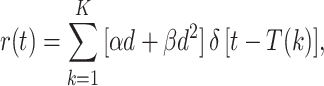 |
19 |
where δ [t] is the Dirac delta function.
Equation (19) corresponds to the statements that on average the surviving cell fraction for the kth dose-fraction is given by (18) and that pre-malignant stem cells have the same radiosensitivity to inactivation as do normal stem cells. By our assumption that, during the comparatively short radiotherapy and recovery periods, normal and pre-malignant cells have effectively the same proliferation rate, the appropriate birth rate is
 |
20 |
In (20) n(t) is a known function of time, determined as discussed above.
It is well known (Tan 2002, pp. 169–171) that by integrating an appropriate partial differential equation for the probability generating function one can deduce the following expression for the probability F(k) that the pre-malignant clone survives all subsequent dose-fractions:
 |
21 |
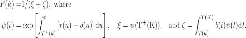
Here, T +(k) denotes the time just after the kth fraction. Because of the way a Dirac δ function behaves, using T + rather than T is important in the expressions for ψ and ξ.
Performing the integrals in (21) with the help of (16–20) gives, after a quite long, but routine, calculation, the following convenient equation for the clone survival probability F(k):
 |
22 |
Equation (22) is valid for k = 0, 1,…, K, with k = 0 referring to pre-malignant cells present before radiation starts and F(K) = 1. It is the primary mathematical result needed for the data analysis discussed in the main text.
We have some extensions, not needed in the present paper. Generalizing to situations where the spontaneous death rate is non-zero and/or one needs the probability that a clone has a given number of cells at the final time, can readily be done by using results given by Tan (2002). In addition, it can be shown that (22) holds even if the recovery equation for normal cells is different from the logistic equation used in this paper, e.g., is Gompertzian.
Footnotes
An erratum to this article is available at http://dx.doi.org/10.1007/s00411-011-0378-5.
Contributor Information
Igor Shuryak, Email: ishuryak@gmail.com.
David J. Brenner, Phone: +1-212-3059930, FAX: +1-212-3053229, Email: djb3@columbia.edu
References
- Armitage P. Multistage models of carcinogenesis. Environ Health Perspect. 1985;63:195–201. doi: 10.2307/3430046. [DOI] [PMC free article] [PubMed] [Google Scholar]
- Armitage P, Doll R. The age distribution of cancer and a multi-stage theory of carcinogenesis. Br J Cancer. 1954;VIII:1–12. doi: 10.1038/bjc.1954.1. [DOI] [PMC free article] [PubMed] [Google Scholar]
- Bennett WR, Crew TE, Slack JM, Ward A. Structural-proliferative units and organ growth: effects of insulin-like growth factor 2 on the growth of colon and skin. Development. 2003;130:1079–1088. doi: 10.1242/dev.00333. [DOI] [PubMed] [Google Scholar]
- Borthwick DW, Shahbazian M, Krantz QT, Dorin JR, Randell SH. Evidence for stem-cell niches in the tracheal epithelium. Am J Respir Cell Mol Biol. 2001;24:662–670. doi: 10.1165/ajrcmb.24.6.4217. [DOI] [PubMed] [Google Scholar]
- Brenner DJ, Curtis RE, Hall EJ, Ron E. Second malignancies in prostate carcinoma patients after radiotherapy compared with surgery. Cancer. 2000;88:398–406. doi: 10.1002/(SICI)1097-0142(20000115)88:2<398::AID-CNCR22>3.0.CO;2-V. [DOI] [PubMed] [Google Scholar]
- Brenner DJ, Shuryak I, Russo S, Sachs RK. Reducing second breast cancers: a potential role for prophylactic mammary irradiation. J Clin Oncol. 2007;25:4868–4872. doi: 10.1200/JCO.2007.11.0379. [DOI] [PubMed] [Google Scholar]
- Brunet A, Rando TA. Ageing: from stem to stern. Nature. 2007;449:288–291. doi: 10.1038/449288a. [DOI] [PubMed] [Google Scholar]
- Campbell F, Williams GT, Appleton MA, Dixon MF, Harris M, Williams ED. Post-irradiation somatic mutation and clonal stabilisation time in the human colon. Gut. 1996;39:569–573. doi: 10.1136/gut.39.4.569. [DOI] [PMC free article] [PubMed] [Google Scholar]
- Carlson ME, Conboy IM. Loss of stem cell regenerative capacity within aged niches. Aging Cell. 2007;6:371–382. doi: 10.1111/j.1474-9726.2007.00286.x. [DOI] [PMC free article] [PubMed] [Google Scholar]
- Dörr W, Kummermehr J. Accelerated repopulation of mouse tongue epithelium during fractionated irradiations or following single doses. Radiother Oncol. 1990;17:249–259. doi: 10.1016/0167-8140(90)90209-F. [DOI] [PubMed] [Google Scholar]
- Editorial (no authors listed) (2004) Cancer survivors: living longer, and now, better. Lancet 364:2153–2154 [DOI] [PubMed]
- Edwards CM, Chapman SJ. Biomechanical modelling of colorectal crypt budding and fission. Bull Math Biol. 2007;69:1927–1942. doi: 10.1007/s11538-007-9199-8. [DOI] [PubMed] [Google Scholar]
- Engquist BLP, Runborg O. Multiscale methods in science and engineering. New York: Springer; 2005. [Google Scholar]
- Fuchs E, Tumbar T, Guasch G. Socializing with the neighbors: stem cells and their niche. Cell. 2004;116:769–778. doi: 10.1016/S0092-8674(04)00255-7. [DOI] [PubMed] [Google Scholar]
- Ghazizadeh S, Taichman LB. Organization of stem cells and their progeny in human epidermis. J Invest Dermatol. 2005;124:367–372. doi: 10.1111/j.0022-202X.2004.23599.x. [DOI] [PMC free article] [PubMed] [Google Scholar]
- Greaves LC, Preston SL, Tadrous PJ, Taylor RW, Barron MJ, Oukrif D, Leedham SJ, Deheragoda M, Sasieni P, Novelli MR, Jankowski JA, Turnbull DM, Wright NA, McDonald SA. Mitochondrial DNA mutations are established in human colonic stem cells, and mutated clones expand by crypt fission. Proc Natl Acad Sci USA. 2006;103:714–719. doi: 10.1073/pnas.0505903103. [DOI] [PMC free article] [PubMed] [Google Scholar]
- Hahnfeldt P, Hlatky L. Cell resensitization during protracted dosing of heterogeneous cell populations. Radiat Res. 1998;150:681–687. doi: 10.2307/3579891. [DOI] [PubMed] [Google Scholar]
- Hanin LG. A stochastic model of tumor response to fractionated radiation: limit theorems and rate of convergence. Math Biosci. 2004;191:1–17. doi: 10.1016/j.mbs.2004.04.003. [DOI] [PubMed] [Google Scholar]
- Heidenreich WF, Hoogenveen R. Limits of applicability for the deterministic approximation of the two-step clonal expansion model. Risk Anal. 2001;21:103–105. doi: 10.1111/0272-4332.211093. [DOI] [PubMed] [Google Scholar]
- Heidenreich WF, Cullings HM, Funamoto S, Paretzke HG. Promoting action of radiation in the atomic bomb survivor carcinogenesis data? Radiat Res. 2007;168:750–756. doi: 10.1667/RR0919.1. [DOI] [PubMed] [Google Scholar]
- Hofmann W, Crawford-Brown DJ, Fakir H, Monchaux G. Modeling lung cancer incidence in rats following exposure to radon progeny. Radiat Prot Dosimetry. 2006;122:345–348. doi: 10.1093/rpd/ncl492. [DOI] [PubMed] [Google Scholar]
- Ivanov VK, Gorski AI, Tsyb AF, Ivanov SI, Naumenko RN, Ivanova LV. Solid cancer incidence among the Chernobyl emergency workers residing in Russia: estimation of radiation risks. Radiat Environ Biophys. 2004;43:35–42. doi: 10.1007/s00411-003-0223-6. [DOI] [PubMed] [Google Scholar]
- Ivanov VK, Gorsky AI, Kashcheev VV, Maksioutov MA, Tumanov KA (2009) Latent period in induction of radiogenic solid tumors in the cohort of emergency workers. Radiat Environ Biophys. doi:10.1007/s00411-009-0223-2 [DOI] [PubMed]
- Johnston MD, Edwards CM, Bodmer WF, Maini PK, Chapman SJ. Mathematical modeling of cell population dynamics in the colonic crypt and in colorectal cancer. Proc Natl Acad Sci USA. 2007;104:4008–4013. doi: 10.1073/pnas.0611179104. [DOI] [PMC free article] [PubMed] [Google Scholar]
- Li L, Xie T. Stem cell niche: structure and function. Annu Rev Cell Dev Biol. 2005;21:605–631. doi: 10.1146/annurev.cellbio.21.012704.131525. [DOI] [PubMed] [Google Scholar]
- Lindsay KA, Wheldon EG, Deehan C, Wheldon TE. Radiation carcinogenesis modelling for risk of treatment-related second tumours following radiotherapy. Br J Radiol. 2001;74:529–536. doi: 10.1259/bjr.74.882.740529. [DOI] [PubMed] [Google Scholar]
- Little MP. A multi-compartment cell repopulation model allowing for inter-compartmental migration following radiation exposure, applied to leukaemia. J Theor Biol. 2007;245:83–97. doi: 10.1016/j.jtbi.2006.09.026. [DOI] [PubMed] [Google Scholar]
- Little MP, Li G. Stochastic modelling of colon cancer: is there a role for genomic instability? Carcinogenesis. 2007;28:479–487. doi: 10.1093/carcin/bgl173. [DOI] [PubMed] [Google Scholar]
- Little MP, Wright EG. A stochastic carcinogenesis model incorporating genomic instability fitted to colon cancer data. Math Biosci. 2003;183:111–134. doi: 10.1016/S0025-5564(03)00040-3. [DOI] [PubMed] [Google Scholar]
- Mebust M, Crawford-Brown D, Hofmann W, Schollnberger H. Testing extrapolation of a biologically based exposure-response model from in vitro to in vivo conditions. Regul Toxicol Pharmacol. 2002;35:72–79. doi: 10.1006/rtph.2001.1516. [DOI] [PubMed] [Google Scholar]
- Moolgavkar SH. The multistage theory of carcinogenesis and the age distribution of cancer in man. J Natl Cancer Inst. 1978;61:49–52. doi: 10.1093/jnci/61.1.49. [DOI] [PubMed] [Google Scholar]
- Moolgavkar S. Multistage models for carcinogenesis. J Natl Cancer Inst. 1980;65:215–216. [PubMed] [Google Scholar]
- Moolgavkar SH, Knudson AG., Jr Mutation and cancer: a model for human carcinogenesis. J Natl Cancer Inst. 1981;66:1037–1052. doi: 10.1093/jnci/66.6.1037. [DOI] [PubMed] [Google Scholar]
- Nordling CO. A new theory on the cancer inducing mechanism. Br J Cancer. 1953;7:68–72. doi: 10.1038/bjc.1953.8. [DOI] [PMC free article] [PubMed] [Google Scholar]
- Pabst S, Spekl K, Dorr W. Changes in the effect of dose fractionation during daily fractionated irradiation: studies in mouse oral mucosa. Int J Radiat Oncol Biol Phys. 2004;58:485–492. doi: 10.1016/j.ijrobp.2003.09.063. [DOI] [PubMed] [Google Scholar]
- Pierce DA, Mendelsohn ML. A model for radiation-related cancer suggested by atomic bomb survivor data. Radiat Res. 1999;152:642–654. doi: 10.2307/3580260. [DOI] [PubMed] [Google Scholar]
- Pierce DA, Vaeth M. Age-time patterns of cancer to be anticipated from exposure to general mutagens. Biostatistics. 2003;4:231–248. doi: 10.1093/biostatistics/4.2.231. [DOI] [PubMed] [Google Scholar]
- Pompei F, Wilson R. A quantitative model of cellular senescence influence on cancer and longevity. Toxicol Ind Health. 2002;18:365–376. doi: 10.1191/0748233702th164oa. [DOI] [PubMed] [Google Scholar]
- Pompei F, Polkanov M, Wilson R. Age distribution of cancer in mice: the incidence turnover at old age. Toxicol Ind Health. 2001;17:7–16. doi: 10.1191/0748233701th091oa. [DOI] [PubMed] [Google Scholar]
- Potten CS, Booth C. Keratinocyte stem cells: a commentary. J Invest Dermatol. 2002;119:888–899. doi: 10.1046/j.1523-1747.2002.00020.x. [DOI] [PubMed] [Google Scholar]
- Radivoyevitch T, Kozubek S, Sachs RK. Biologically based risk estimation for radiation-induced CML. Inferences from BCR and ABL geometric distributions. Radiat Environ Biophys. 2001;40:1–9. doi: 10.1007/s004110100088. [DOI] [PubMed] [Google Scholar]
- Ritter G, Wilson R, Pompei F, Burmistrov D. The multistage model of cancer development: some implications. Toxicol Ind Health. 2003;19:125–145. doi: 10.1191/0748233703th195oa. [DOI] [PubMed] [Google Scholar]
- Ron E. Childhood cancer—treatment at a cost. J Natl Cancer Inst. 2006;98:1510–1511. doi: 10.1093/jnci/djj437. [DOI] [PubMed] [Google Scholar]
- Sachs RK, Brenner DJ. Solid tumor risks after high doses of ionizing radiation. Proc Natl Acad Sci USA. 2005;102:13040–13045. doi: 10.1073/pnas.0506648102. [DOI] [PMC free article] [PubMed] [Google Scholar]
- Sachs RK, Chan M, Hlatky L, Hahnfeldt P. Modeling intercellular interactions during carcinogenesis. Radiat Res. 2005;164:324–331. doi: 10.1667/RR3413.1. [DOI] [PubMed] [Google Scholar]
- Sachs RK, Shuryak I, Brenner D, Fakir H, Hlatky L, Hahnfeldt P. Second cancers after fractionated radiotherapy: stochastic population dynamics effects. J Theor Biol. 2007;249:518–531. doi: 10.1016/j.jtbi.2007.07.034. [DOI] [PMC free article] [PubMed] [Google Scholar]
- Schneider U, Walsh L. Cancer risk estimates from the combined Japanese A-bomb and Hodgkin cohorts for doses relevant to radiotherapy. Radiat Environ Biophys. 2008;47:253–263. doi: 10.1007/s00411-007-0151-y. [DOI] [PubMed] [Google Scholar]
- Schollnberger H, Mitchel RE, Azzam EI, Crawford-Brown DJ, Hofmann W. Explanation of protective effects of low doses of gamma-radiation with a mechanistic radiobiological model. Int J Radiat Biol. 2002;78:1159–1173. doi: 10.1080/0955300021000034693. [DOI] [PubMed] [Google Scholar]
- Sharpless NE, DePinho RA. How stem cells age and why this makes us grow old. Nat Rev Mol Cell Biol. 2007;8:703–713. doi: 10.1038/nrm2241. [DOI] [PubMed] [Google Scholar]
- Shuryak I, Sachs RK, Hlatky L, Little MP, Hahnfeldt P, Brenner DJ. Radiation-induced leukemia at doses relevant to radiation therapy: modeling mechanisms and estimating risks. J Natl Cancer Inst. 2006;98:1794–1806. doi: 10.1093/jnci/djj497. [DOI] [PubMed] [Google Scholar]
- Shuryak I, Hahnfeldt P, Hlatky L, Sachs RK, Brenner DJ (2009) A new view of radiation-induced cancer: integrating short- and long-term processes. Part II: Second cancer risk estimation. Radiat Environ Biophys. doi:10.1007/s00411-009-0231-2 [DOI] [PMC free article] [PubMed]
- Slack JM. Stem cells in epithelial tissues. Science. 2000;287:1431–1433. doi: 10.1126/science.287.5457.1431. [DOI] [PubMed] [Google Scholar]
- Spencer SL, Gerety RA, Pienta KJ, Forrest S. Modeling somatic evolution in tumorigenesis. PLoS Comput Biol. 2006;2:e108. doi: 10.1371/journal.pcbi.0020108. [DOI] [PMC free article] [PubMed] [Google Scholar]
- Tan W. Stochastic models with applications to genetics, cancers, AIDS, and other biomedical systems. London: World Scientific; 2002. [Google Scholar]
- Tokunaga M, Norman JE, Jr, Asano M, Tokuoka S, Ezaki H, Nishimori I, Tsuji Y. Malignant breast tumors among atomic bomb survivors, Hiroshima and Nagasaki, 1950–74. J Natl Cancer Inst. 1979;62:1347–1359. [PubMed] [Google Scholar]
- Travis LB, Curtis RE, Boice JD, Jr, Platz CE, Hankey BF, Fraumeni JF., Jr Second malignant neoplasms among long-term survivors of ovarian cancer. Cancer Res. 1996;56:1564–1570. [PubMed] [Google Scholar]
- Travis LB, Curtis RE, Storm H, Hall P, Holowaty E, Van Leeuwen FE, Kohler BA, Pukkala E, Lynch CF, Andersson M, Bergfeldt K, Clarke EA, Wiklund T, Stoter G, Gospodarowicz M, Sturgeon J, Fraumeni JF, Jr, Boice JD., Jr Risk of second malignant neoplasms among long-term survivors of testicular cancer. J Natl Cancer Inst. 1997;89:1429–1439. doi: 10.1093/jnci/89.19.1429. [DOI] [PubMed] [Google Scholar]
- Travis LB, Gospodarowicz M, Curtis RE, Clarke EA, Andersson M, Glimelius B, Joensuu T, Lynch CF, van Leeuwen FE, Holowaty E, Storm H, Glimelius I, Pukkala E, Stovall M, Fraumeni JF, Jr, Boice JD, Jr, Gilbert E. Lung cancer following chemotherapy and radiotherapy for Hodgkin’s disease. J Natl Cancer Inst. 2002;94:182–192. doi: 10.1093/jnci/94.3.182. [DOI] [PubMed] [Google Scholar]
- Travis LB, Hill DA, Dores GM, Gospodarowicz M, van Leeuwen FE, Holowaty E, Glimelius B, Andersson M, Wiklund T, Lynch CF, Van’t Veer MB, Glimelius I, Storm H, Pukkala E, Stovall M, Curtis R, Boice JD, Jr, Gilbert E. Breast cancer following radiotherapy and chemotherapy among young women with Hodgkin disease. JAMA. 2003;290:465–475. doi: 10.1001/jama.290.4.465. [DOI] [PubMed] [Google Scholar]
- Travis LB, Fossa SD, Schonfeld SJ, McMaster ML, Lynch CF, Storm H, Hall P, Holowaty E, Andersen A, Pukkala E, Andersson M, Kaijser M, Gospodarowicz M, Joensuu T, Cohen RJ, Boice JD, Jr, Dores GM, Gilbert ES. Second cancers among 40, 576 testicular cancer patients: focus on long-term survivors. J Natl Cancer Inst. 2005;97:1354–1365. doi: 10.1093/jnci/dji278. [DOI] [PubMed] [Google Scholar]
- Ullrich RL. The rate of progression of radiation-transformed mammary epithelial cells is enhanced after low-dose-rate neutron irradiation. Radiat Res. 1986;105:68–75. doi: 10.2307/3576726. [DOI] [PubMed] [Google Scholar]
- van Leeuwen FE, Klokman WJ, Stovall M, Dahler EC, van’t Veer MB, Noordijk EM, Crommelin MA, Aleman BM, Broeks A, Gospodarowicz M, Travis LB, Russell NS. Roles of radiation dose, chemotherapy, and hormonal factors in breast cancer following Hodgkin’s disease. J Natl Cancer Inst. 2003;95:971–980. doi: 10.1093/jnci/95.13.971. [DOI] [PubMed] [Google Scholar]
- Wheldon EG, Lindsay KA, Wheldon TE. The dose-response relationship for cancer incidence in a two-stage radiation carcinogenesis model incorporating cellular repopulation. Int J Radiat Biol. 2000;76:699–710. doi: 10.1080/095530000138376. [DOI] [PubMed] [Google Scholar]
- Yakovlev A, Polig E. A diversity of responses displayed by a stochastic model of radiation carcinogenesis allowing for cell death. Math Biosci. 1996;132:1–33. doi: 10.1016/0025-5564(95)00047-X. [DOI] [PubMed] [Google Scholar]
- Zhang W, Remenyik E, Zelterman D, Brash DE, Wikonkal NM. Escaping the stem cell compartment: sustained UVB exposure allows p53-mutant keratinocytes to colonize adjacent epidermal proliferating units without incurring additional mutations. Proc Natl Acad Sci USA. 2001;98:13948–13953. doi: 10.1073/pnas.241353198. [DOI] [PMC free article] [PubMed] [Google Scholar]