

Abstract
The Helmholtz free energy, F and the entropy, S are related thermodynamic quantities with a special importance in structural biology. We describe the difficulties in calculating these quantities and review recent methodological developments. Because protein flexibility is essential for function and ligand binding, we discuss the related problems involved in the definition, simulation, and free energy calculation of microstates (such as the α-helical region of a peptide). While the review is broad, a special emphasize is given to methods for calculating the absolute F (S), where our HSMC(D) method is described in some detail.
I.Introduction
The absolute entropy, S and the absolute Helmholtz free energy, F (or G – Gibbs free energy) are fundamental quantities in statistical mechanics with a special importance in structural biology. S is a measure of order where changes in the S of water lead to the hydrophobic interaction – the main driving force in protein folding. F constitutes the criterion of stability, which is essential for studying the structure and function of peptides, proteins, nucleic acids, and other biological macromolecules. The free energy defines the binding affinities of protein-protein and protein-ligand interactions, it also quantifies many other important processes such as enzymatic reactions, electron transfer, ion transport through membranes, and the solvation of small molecules.
However, calculation of F(S) by computer simulation is extremely difficult, and considerable attention has thus been devoted in the last 50 years to this subject. While significant progress has been made (see reviews in [1-9]), in many cases the efficiency (or accuracy) of existing methods is unsatisfactory and the need for new ideas has kept this field highly active. We summarize here mainly recent developments in this area of research where the emphasis is on methodology issues and less on applications. The present article constitutes a substantial extension of a concise review appeared recently [7].
II. General theoretical considerations
In this section we define various thermodynamic quantities and discuss the problems involved in estimating them by computer simulation.
II.1 Statistical mechanics
The commonly used simulation techniques, Metropolis Monte Carlo (MC) [10] and molecular dynamics (MD) [11,12] are exact methods which enable one to generate samples of system configurations i distributed according to the Boltzmann probability, PiB (for simplicity we discuss a discrete system such as a lattice model of N particles),
| (1) |
where T is the absolute temperature, kB is the Boltzmann constant and Ei is the potential energy of configuration i; Z is the configurational partition function.
| (2) |
where the summation (integration for a continuum system) is carried out over the entire ensemble of configurations. The ensemble averages of the energy, <E>, and the absolute entropy, S, are given by
| (3) |
and
| (4) |
where the free energy, F, can also be expressed (formally) as an ensemble average,
| (5) |
An extremely important property of this representation of F (but not of other representations) is that its variance vanishes, σ2(F)=0; indeed, substituting the expression for PiB [equation (1)] in the brackets [equation (5)] leads to a constant, -kBTlnZ for any i [13,14]. This means that the exact free energy can be obtained from any single structure i if PiB is known. Moreover, while F is an extensive variable, its zero fluctuation property holds for any number of atoms N. This important property is not shared by the entropy and the energy - their fluctuations increase as ∼N1/2, which makes it difficult to calculate small entropy and energy changes [see discussion following equation (25)]. <E> can be estimated from a sample of size n generated with MC or MD (i.e., with the correct Boltzmann probability) by the arithmetic average, E̅
| (6) |
where the values of Et are easily measured for each of the sampled configurations (e.g, the sum of the Lennard-Jones interactions for argon). (One has to distinguish between a summation over the entire ensemble which is denoted by the index i and a summation over a sample of n configurations which is denoted by the index t.) On the other hand, estimation of S by S̅,
| (7) |
is not straightforward because (unlike the energy) the value of ln PtB is not “written” directly on each of the sampled configuration, rather, it is a function of the entire ensemble through Z [equation (2)]; moreover, Z is not provided by the MC and MD simulation methods (methods which are of a “dynamic type”). The difficulty in calculating F stems from the relation F=E-TS.
II.2 The free energy of a partial region of space
The above discussion in terms of a discrete system also holds for a continuum system where the potential energy is E(x), x ∈ Ω is a 3N-dimensional vector of the Cartesian coordinates of the N atoms, and Ω is the entire configurational space. Thus, the summations (over the entire ensemble) are replaced by integrations over Ω. Moreover, this theory also applies to any partial region Ωm of Ω, where a corresponding partial free energy, Fm can be defined,
| (8) |
Notice that the integral defining Zm has the dimension of x, hence Fm and Sm are defined up to an additive term ∼lnx (which disappears if the velocity part of the partition function is considered). However, in most cases one is mainly interested in differences ΔFmn and ΔSmn for a system in regions Ωm and Ωn at a given T, where the additive factors are cancelled. Correspondingly, the dependence on dimensionality is cancelled in the ratio of populations, pm/pn (pm=exp[–Fm/kBT]/Z) which is much easier to calculate than the populations themselves,
| (9) |
II.3 Microstates and intermediate flexibility
While the difficulty in calculating the absolute S (F) discussed above is common to all systems, biological macromolecules such as peptides and proteins, are particularly challenging due to their rugged potential energy surface, E(x). More specifically, this surface is “decorated” by a tremendous number of localized energy wells and “wider” ones that are defined over microstates (regions Ωm), each consisting of many localized wells (Fig. 1); a microstate can be represented by a sample (trajectory) generated by a local MD simulation (e.g., the α-helical region of a peptide, see further discussion in II.4 below). MD studies have shown that a molecule will visit a localized well only for a very short time (as short as several fs) while staying for a much longer time within a microstate [15,16], meaning that the microstates are of a greater physical significance than the localized wells. A central aim of computational structural biology is to fold a protein, i.e., to identify its (single) Ωm with global minimum Fm (out of trillions of microstates) – an unsolved optimization task. It is noted further that Fm of non-stable microstates, such as a transition state, might also be of interest.
Figure (1).

Schematic one-dimensional representation of part of the energy surface of a peptide or a protein, as a function of a coordinate X. The two large potential energy wells are defined over the corresponding microstates denoted Ω1 and Ω2. Each microstate consists of many localized potential wells denoted intermittently by solid and dashed lines. The partition function Zm of microstate m is obtained by integrating exp[-E/kBT] over Ωm where Fm = - kBT lnZm is the microstate's free energy. The figure suggests that the second microstate is the more stable among the two due to lower energy and higher entropy (Ω2 is larger than Ω1) hence lower free energy. If F2 is also the global free energy minimum of a protein, Ω2 is expected to describe the native microstate (assuming a perfect force field) and a simulation started from Ω2 will keep the protein in this microstate for a long time. On the other hand, a peptide can populate significantly several of the most stable microstates in thermodynamic equilibrium.
Free energy calculations are also required in problems which are less challenging than protein folding, i.e., in cases of intermediate flexibility, where a flexible protein segment (e.g., a side chain or a surface loop), a cyclic peptide, or a ligand bound to an enzyme populates significantly several microstates in thermodynamic equilibrium. It is of interest, for example, to know whether the conformational change adopted by a loop (a side chain, ligand, etc.) upon protein binding has been induced by the other protein (induced fit [17,18]) or alternatively the free loop already interconverts among different microstates where one of them is selected upon binding (selected fit [19]). This analysis requires calculating the relative populations, pm/pn [equation (9)], which are also needed for a correct analysis of nuclear magnetic resonance (NMR) and x-ray data of flexible macromolecules [20,21].
II.4 On the practical definition of a microstate
Calculating populations, pm or ratios pm/pn by the various techniques cannot be achieved without first establishing a practical definition of a microstate, which is however not trivial. Therefore, we elaborate below about this important issue that has been ignored to a large extent in the literature but has been given considerable thought by us over the course of the years [22-32]. For simplicity we consider an N-residue peptide with rigid geometry, i.e., constant bond lengths and bond angles meaning that its backbone conformation is solely defined by the dihedral angles, φk and ψk, where k=1,N. (ωk, for the peptide bond, is fixed at 180°.) For a helical microstate (Ωh), these angles are expected to vary within relatively small ranges Δφk and Δψk around φk = -60° and ψk = -50° (we ignore for a moment the side chains). However, if N is not too small, the correct limits of Ωh in the [φk,ψk] space are unknown even for this simplified model since they constitute a complicated narrow “pipe” contained within the (larger) region defined by the product, Δφ1×Δψ1×Δφ2×Δψ2 ····· ΔφN×ΔψN due to the strong correlations among the dihedral angles. Obviously, these correlations are taken into account by an exact simulation method and thus, in practice, Ωh can be defined (or more correctly, represented) by a local MC (MD) sample of conformations initiated from an α-helical structure, as mentioned earlier.
However, this definition should be used with caution. Thus, a short simulation will span only a small part of Ωh and this part will grow constantly as the simulation continues; correspondingly, the calculated average potential energy, Eh and the entropy Sh (obtained by any method) will both increase and the free energy, Fh is expected to change as well. As the simulation time is increased further, side chain dihedrals will “jump” to different rotamers, which according to our definition should also be included within Ωh; for a long enough simulation the peptide is expected to “leave” the α-helical region and move to a different microstate. Thus, in practice, the microstate size and the corresponding thermodynamic quantities can depend on the simulation time used to define the microstate. In some cases, one can better define Ωh by discarding structures with dihedral angles beyond predefined Δφk and Δψk values or structures that do not satisfy a certain number of hydrogen bonds; one can also apply energetic restraints where their bias should be removed. However, these restrictions are somewhat arbitrary and are difficult to apply for calculating the differences ΔFmn and ΔSmn between microstates Ωm and Ωn, which is our main interest. Therefore, one should bear in mind that in practice there is always some arbitrariness in the definition of a microstate, which affects the calculated averages. This arbitrariness is severe with some methods and can be controlled (minimized) by others, as is discussed in the coming sections.
III. Methods for calculating the free energy
The various methods are divided into three main categories, the “counting approach”, thermodynamic integration/perturbation, and methods for calculating the absolute F and S. For brevity in what follows we denote microstates by m and n rather than by Ωm and Ωn.
III.1 The counting approach
As has been already pointed out, in many cases one is interested in differences ΔSmn and ΔFmn (or Zm/Zn) between two microstates (and less in S and F themselves). ΔFmn can be calculated in the most straightforward way by a counting method, i.e., from a long MD (or MC) simulation that “covers” both microstates, where
| (10) |
and #m (#n) is the number of times the molecule visited m (n) during the simulation. However, because of high energy barriers, the transition between microstates at room temperature might require long times, nanoseconds or more even for side chain rotamers, meaning that reliable sampling of #m (#n) might become prohibitive. This problem can be alleviated by applying enhanced sampling techniques such as replica exchange [33] or the multicanonical method [34,35]; however, the conformational search capability of these methods is also limited and microstates of interest might be visited poorly (or not at all). The common analysis is based on projecting MD (MC) trajectories onto a small number of coordinates using principal component analysis, PCA (to help define/identify microstates), or in simpler cases calculating the populations along one or two physically significant reaction coordinates [36,37].
III.2 The thermodynamic integration approach
Differences ΔF and ΔS are commonly calculated by thermodynamic integration (TI) over physical quantities such as the energy, temperature, pressure, specific heat, etc. [38,39], as well as non-physical parameters, for instance, using a coupling parameter to act on the interaction potential to effect an “alchemical mutation”. In addition to TI, free energy perturbation (FEP) [1-9,40-47] and histogram analysis methods [48-50] can also be applied and will be included in this category. These are robust and highly versatile approaches, which have been reviewed extensively [1-9] and therefore only recent developments will be discussed here, some of them in detail.
III.2.a Advantages of TI and some pitfalls
An important application of TI is calculating the difference in the binding free energy of two ligands a and b bound to a protein (or a single ligand bound to a protein before or after a mutation in the protein). In this case two different simulations (integrations) are carried out in which a is mutated to b in water (aw→bw) and in the protein environment (Pa→Pb), and the corresponding differences in free energy, ΔFaw→bw and ΔFPa→Pb are obtained. Because the free energy generated during a reversible thermodynamic cycle is zero, one can obtain the required overall difference in the binding free energy (see Fig. 2),
Figure (2).

A thermodynamic cycle for the binding of two ligands a and b to a protein P. In the experiment the ligands are transferred from the solvent to the active site where one measures the difference ΔΔF = ΔFaw →Pa - ΔFbw →Pb. In simulations the nonphysical transformation a→b is carried out in the protein and in solution and the corresponding free energies ΔFPa→Pb and ΔFaw →bw are calculated. Because the free energy of the entire cycle is zero, the desired ΔΔF is obtained in terms of the nonphysical free energy differences ΔΔF = ΔFPa→Pb - ΔFaw →bw.
| (11) |
This procedure is extremely valuable because it enables one to calculate small free energy differences, ΔFaw→bw and ΔFPa→Pb in large systems - a large container of water, and a large protein solvated by water. This stems from the fact that during the TI process only the interactions of the relatively small mutated part of the ligand with the system is directly considered (in the relevant derivatives to be integrated) and the resulting fluctuations are therefore small; on the other hand, obtaining ΔFaw→bw (and ΔFPa→Pb) from ΔEaw→bw - TΔSaw→bw would be prohibitive, because both the energy and entropy depend on all of the system interactions, the fluctuations are large (∼N1/2), and in practice the high precision required is not achievable [51-53].
However, TI has weaknesses that should be emphasized. Thus, if one seeks to calculate ΔFmn between microstates m and n with significant structural variance (e.g., a helix and a hairpin of a peptide) the integration becomes difficult (due to the complex path), and for a large molecule unfeasible. This difficulty may also be problematic in the calculation of the free energy of binding described above. Thus, whereas the mutation of a to b in the more homogeneous solvent environment might be well controlled, the simulation in the protein environment might not converge for very long times due to conformational changes (e.g., “jumps” of side chains among rotamers, etc.) occurring constantly in the entire protein; in other words, the microstate of Pb (and to some extent also of Pa) keep changing as the simulation time increases. Also, sometimes the mutation process does not lead to the required size and shape of the active site of Pb, or to the correct position of b and the correct number of water molecules in the active site of Pb [54,55].
As discussed below, these drawbacks can be overcome to a large extent with methods that calculate the absolute free energy. In this context it should be pointed out that the absolute F can also be obtained with TI provided that a reference state R with known F is available and an efficient integration path R→m can be defined. A classic example is the calculation of F of liquid argon or water by integrating the free energy from an ideal gas reference state. However, for non-homogeneous systems such integration might not be trivial, and in models of peptides and proteins defining adequate reference states is not straightforward (see later discussions in III.3.b.7). However, in spite of these problems, the TI approach is applied regularly for calculating the free energy of binding (and other properties) and the required computer programs are implemented in the commonly used molecular mechanics/molecular dynamics software packages, such as AMBER [56], CHARMM [57], NAMD [58], BOSS [59], GROMOS [60], GROMACS [61], TINKER [62], and others.
III.2.b The Adaptive Integration Method
An interesting development in the TI category is the Adaptive Integration Method (AIM) for computing free energies, radial distribution functions, and potentials of mean force [63]. A general TI process is based on the integral
| (12) |
where 0 ≤ λ ≤ 1 defines a hybrid Hamiltonian, H(λ) = (1- λ)U0 + λU1, that is varied between two energy functions U0 and U1. (H(λ) can also be defined by more general nonlinear scalings.) This integral is commonly evaluated by carrying out l separate MD (or MC) simulations at l intermediate λ values, where the l corresponding averages (in conformational space x) of the derivative <dH(λ,x)/dλ>λ = <U1-U0>λ are calculated. With AIM, on the other hand, the sampling is performed within an MC procedure that allows transitions between coordinates as well as between different λ values. The parameter, λ, is therefore treated as an additional coordinate thus defining an expanded (λ,x) “super-system”. Thus, if the (a-priori unknown) partition function at λ is Zλ (Zλ = ∫ exp[−H(λ,x)/kBT]dx), a normalized (Boltzmann) probability for the super-system to be at (λ,x) can be defined as
| (13) |
Note that each λ value has been weighted (by 1/Zλ) to give the same probability, PB(λ)=1/{Σλ′∫exp[-H(λ′,x)/kBT]dx/Zλ′}. The MC transition probabilities should satisfy the detailed balance condition, p(λ1→ λ2) / p(λ2→ λ1)=PB(λ2,x)/ PB(λ1,x), which leads to
| (14) |
Because Zλ is not known a-priori, the free energy, F̅λ = −kBT ln Z̅λ in equation (14) is approximate and therefore appears with a bar. The values of F̅λ (Z̅λ) are calculated with an adaptive procedure. In particular, the transition probabilities (equation (14)) are estimated by using the current (running) estimates for the free energy derivatives, <dH(λ,x)/dλ>λ, wherein, the free energy difference, , is thus approximated by a simple numerical integration. As the simulation continues, the running averages of the free energy derivatives become more accurate, making the estimated free energy differences increasingly accurate, and thus, the detailed balance condition will be satisfied (albeit asymptotically) with all λ values (bins) being visited an equal number of times. In a more traditional way for estimating F̅λ, the simulation starts with Z̅λ = 1 for all λ, where for each visit of a λ value Z̅λ is increased by 1, and the simulation continues with the current (updated) Z̅λ; thus, asymptotically (i.e., for a very long run) the ratios of the Z̅λ values attain stability, Z̅λi/Z̅λj ≈ Z̅λi/Z̅λj. Notice also that for each λ the transitions between the coordinates (x) can be carried out by any canonical simulation technique (MC, MD etc.).
The authors claim that a larger number of bins (λ values) can be treated with AIM than with TI (for the same amount of computer time) which leads to a much finer resolution. Another potential advantage of AIM lies in the fact that a bin might be visited many times during the simulation, each visit starts from a different structure (seed) leading to an adequate sampling of the contributing microstate(s) for this λ. With TI, on the other hand, only a single simulation (starting from one seed) is typically performed and the coverage of the contributing microstates is expected to be more limited.
It should be pointed out that simulation techniques based on an adaptive calculation of (relative) free energies and entropies have been suggested before, starting with the multicanonical technique of Berg and Neuhaus [34], the method of expanded ensembles of Lyubartsev et al. [64], and the simulated tempering method of Marinari and Parisi [65]. The more recent (and relatively simple) random walk algorithm of Wang and Landau [66] has been used extensively, and has become the basis for more sophisticated techniques developed, for example, by de Pablo's group [67-69]. Also, to enhance efficiency, Escobedo and collaborators have devised methods [70-74], which combine the expanded ensembles idea with other known procedures (e.g., Bennett's method [75]). However, unlike AIM, which is aimed at calculating the free energy, most of these methods are designed primarily as simulation tools that enable a system with a rugged energy surface to cross energy barriers efficiently, while differences in free energy (or entropy) are obtained (like other properties) as byproducts of the simulation. A detailed discussion of these methods is beyond the scope of this review and extensive relevant literature can be found in the references cited above. Finally, it should be pointed out that further development of multicanonical ideas has also been pursued by the groups of Okamoto and Nakamura (also for MD simulations) and this approach has been applied extensively to peptides and proteins in explicit water (see for example [76-82] and references cited therein).
III.2.c Methods based on Jarzynski's identity
Another approach for calculating the (reversible) ΔF is based on Jarzynski's identity [47],
| (15) |
where <⋯>0 represents an average over non-reversible forward-directed work values, Wf, generated by starting an equilibrium simulation at U0 which ends at U1. However, if the transformation from U0 to U1 is rapid, a large number of these non-equilibrium simulations must be generated in order to sample the rare, most-contributing paths with low work values. Therefore, increasing efficiency has been a central aim, e.g., by biasing the selection of paths [83-89] or developing alternatives to Jarzynski's identity [90]. Notice however, that these procedures have been tested mostly on highly simplified models.
Shirts and Pande [91] reviewed and developed theoretical estimates for the bias and variance of Jarzynski's identity, TI, and Bennett's method [75]. They applied these methods to toy models but could not define a preferred method for calculating ΔF; however, in applications to simple atomistic models the lowest variance and bias were obtained with Bennett's method. Pande's group also developed efficient methods for calculating the absolute F of binding [92]. In a recent study [93] the accuracy and precision of nine free energy methods have been compared, where among them are, TI, AIM, FEP, Bennett's method, and single-ensemble path sampling [84]. ΔF was calculated for growing a (neutral) Lennard-Jones sphere in water and for charging a Lennard-Jones sphere in water. The efficiency was found to depend on the system and extent of accuracy sought, where overall AIM is the most efficient. Jarzynski's identity was also applied to realistic systems of proteins [94], where steered MD was used for calculating potential of mean force for unbinding acetylcholine from the alpha7 nicotinic acetylcholine receptor ligand-binding domain; four different procedures were checked in this study (see also [95]).
III.3 Calculations of the absolute S and F
Problems associated with the free energy difference-based approaches discussed earlier (e.g., TI) can be remedied to a large extent by calculating the absolute free energy; then, Fm and Fn can be obtained directly from two separate MD (MC) simulations of m and n, which leads to ΔFmn = Fm – Fn and the need for an integration from m to n (or a long simulation that covers both m and n, as in the counting method) is avoided. Several methods have been developed in this category.
III.3.a Harmonic and quasi-harmonic techniques
A commonly used approach for estimating the absolute S is based on the harmonic approximation which was introduced to biomolecules by Gō and Scheraga [96,97]. They obtained
| (16) |
where Hessian is the matrix of second derivatives of the force field with respect to internal coordinates around an energy minimized structure; the quantum mechanical version (Einstein oscillators) was applied later for peptides by Hagler's group [98]. A related approach, “the second generation mining minima” method (M2) [99,100] has been developed by Gilson's group. With M2, low energy minimized structures (within a microstate) are initially identified, the free energies of the corresponding local potential wells are calculated with a method that considers both harmonic and an-harmonic effects, and the contribution of the individual wells is then accumulated.
An important development has been the introduction of the quasiharmonic (QH) method by Karplus and Kushick [101], where the Boltzmann probability density of structures defining a microstate is approximated by a multivariate Gaussian. Thus,
| (17) |
where the covariance matrix, σ, is obtained from a local MD (MC) sample and N is (usually) the number of internal coordinates. Clearly, SQH constitutes an upper bound for S since correlations higher than quadratic are neglected; also, an-harmonic contributions are ignored, and QH is not suitable for diffusive systems such as water.
While QH has been used extensively during the years (see [102-104] and references cited therein), a systematic study of its performance has been carried out only recently by Gilson's group [105]. They studied linear alkanes and a host-guest system (urea receptor with the ethylenurea ligand) comparing the QH results to those obtained by the M2 method mentioned above. The conclusions of this study are that QH can be accurate for a highly populated single energy well, where the calculation is based on internal coordinates; the use of Cartesians, however, leads to errors of several kcal/mol. When the simulation covers several energy wells the errors of QH (in internal coordinates) can increase to tens of kcal/mol and are significantly larger with QH(Cartesians). Also, while errors sometimes get cancelled in entropy differences, the host-guest studies have shown that the errors in ΔSQH are substantial. Finally, the convergence of the QH results is slow and in the host-guest system convergence has not been obtained even with 6 ns MD runs, which is in accord with previous studies. These conclusions probably apply to other versions of QH where σ is defined in Cartesian coordinates, such as the ad-hoc quantum mechanical approximation of Schlitter [106,103] and the exact derivation of quantum mechanical QH [107]; the performance of these two methods has been compared [108].
A new version of QH has been suggested recently by Wang and Brüschweiler [109], which enables one to estimate the contribution of different potential wells, e.g. rotameric states. Thus, defining a peptide conformation by the dihedral angles θj, a PCA analysis is carried out for a sample of conformations with respect to the complex variables (rather than θj) which eliminates the modulo 2 ambiguity in θj. The sample conformations (defined by the ) are then projected onto each of the eigenvectors m and the distribution of the resulting (complex) values leads to an entropy Sm. In practice, however, these distributions are smoothed by Gaussian functions, which depend on a variance parameter, σ. The total 2D entropy is S2D= Σ Sm (up to an additive factor that controls to a large extent the effect of σ). The method was applied to several simplified models and the protein ubiquitin described by a force field. More recently this technique and the counting method were applied to the second β-hairpin of the B1 domain of streptococcal protein G, and the entropy results of these calculations were found to agree [110].
III.3.b Step-by-step reconstruction methods
Another approach for calculating the absolute S (F) has been suggested by Meirovitch and has been implemented initially in two approximate techniques of general applicability (i.e., not restricted to harmonic conditions), the local states (LS) [111,22-28] and the hypothetical scanning (HS) methods [112,115]. With both methods each conformation i of a sample [generated by MC or MD] is reconstructed step-by-step (from nothing) using transition probabilities (TPs); the product of these TPs leads to an approximation Pi for the correct PiB [equation (1)]. Recently, HS has been developed further to become the HSMC(D) method, where the approximate deterministic calculation of TP(HS) was replaced by a stochastic calculation carried out by MC(MD) simulations [116-121,29-32].
The philosophy of this approach is based on the ideas of the exact scanning method, which is thus described first [122,123]. While these methods are applicable to a wide range of systems, they are described here as applied to a simple peptide – a polyglycine molecule of N residues where its conformations are defined by the dihedral angles φi,ψi, and ωi and the corresponding bond angles (bond lengths are assumed to be constant). These angles ordered along the chain are denoted by αk, k=1,6N and the peptide is assumed to be in the helical microstate, Ωh (however, the conclusions apply to any microstate Ωm.) The potential energy of the peptide is defined by a force field in vacuum.
III.3.b.1 The exact scanning procedure
The exact scanning method [122,123] is a step-by-step construction procedure for a peptide conformation based on calculating (consecutively) TPs for the αk, and determining their values and the positions of the related atoms [124]. For example, the angle φ defines the coordinates of the two hydrogens connected to Cα, and the position of C′. Thus, at step k (starting from nothing), k-1 angles α1, …,αk-1 have already been determined and the related structure (the past) is kept constant. αk is defined with the exact TP density ρ(αk|αk−1,⋯, α1)
| (18) |
That is, ρ(αk|αk−1,⋯, α1)dαk is the probability for the kth angle to be found within a small increment, dαk, centered at αk, given that the angles, 1 through k-1, are at values α1, …, αk-1. Zfuture(αk,⋯,α1) is a “future partition function” where the term “future” indicates that the integration defining Zfuture is carried out over the variables αk+1,⋯, α6N which will be determined only in the future steps of the build-up process. (Similarly, Zfuture(αk−1,⋯,α1) is an integration over the angles αk,⋯, α6N.) In these integrations the atoms treated in the past are held fixed at their respective coordinates. More specifically, for Zfuture(αk,⋯,α1), α1⋯αk are fixed, while αk+1,⋯, α6N are varied in a restrictive way where the corresponding conformations of the “future” part remain within Ωh, and thus we write,
| (19) |
The product of the TPs [equation (18)] leads to the (Boltzmann) probability density of the entire conformation [equation (1)],
| (20) |
This construction procedure is not feasible for a large molecule because the scanning range grows exponentially and the helical region is not known, as discussed in II.4; therefore this method was used as a conformational search technique, where only a limited number of future angles were scanned [124]. However, the ideas of the exact scanning method constitute the basis for the three methods, HS, HSMC(D), and LS, as discussed below.
III.3.b.2 The philosophy of the hypothetical scanning approach
The exact scanning method is equivalent to any other exact simulation technique (in particular MC and MD) in the sense that large samples generated by such methods lead to the same averages and fluctuations within the statistical errors. Therefore, one can assume that a given MC or MD sample has rather been generated by the exact scanning method, which enables one to reconstruct each conformation i by calculating the TP densities that hypothetically were used to create it step-by-step. This idea has been implemented initially in two different ways in the LS and HS methods. However, an exact reconstruction of the TPs [equation (18)] is feasible only for a very small peptide. Therefore, calculation of future partition functions [equation (19)] by these methods has been carried out only approximately, by considering a partial future (or a limited past in the case of LS) as discussed in III.3.b.5. On the other hand, with HSMC(D) the entire future is considered and in this respect HSMC(D) can be considered to be exact.
III.3.b.3 The HSMC(D) method
Because HSMC and HSMD are based on the same theoretical grounds, we denote the related probability functions by ‘HS’, where the theory is described for HSMD, which for peptides has been found to be the more practical and efficient method among the two. One starts by generating an MD sample of the helical microstate; the conformations are then represented in terms dihedral and bond angles,1≤ αk ≤ 6N, and the variability range Δαk is calculated,
| (21) |
where αk(max) and αk(min) are the maximum and minimum values of αk found in the sample, respectively. Δαk, αk(max), and αk(min) enable one to verify that the sample spans correctly the Ωh microstate.
As mentioned in III.3.b.2, with our approach a sample conformation i is reconstructed step-by-step by calculating the TP density of each αk [equation (18)] from the future partition functions Zfuture [equation (19)]. However, a systematic integration of Zfuture based on the entire future within the limits of Ωh is difficult and becomes impractical for a large peptide where Ωh is unknown (see II.4). The idea of the HSMD method is to obtain the TPs [equation (18)] by carrying out MD simulations of the future part of the chain rather than by evaluating the integrals defining Zfuture [equation (19)] in a deterministic way. Thus, at reconstruction step k of conformation i the TP density, ρ(αk|αk−1,⋯,αk) is calculated from an MD sample of nf conformations (generated, in practice, in Cartesian coordinates), where the entire future of the peptide is moved (i.e., the atoms defined by αk,⋯,α6N) while the past (the atoms defined by α1,⋯,αk−1) are kept fixed at their values in conformation i. A small segment (bin) δαk [see also equation (18)] is centered at αk(i) and nvisit, the number of visits of the future chain to this bin during the simulation is calculated; one obtains,
| (22) |
where the relation becomes exact for very large nf (nf → ∞) and a very small bin (δαk→ 0) (see [32]). This means that in practice ρHS(αk|αk−1,⋯,α1 will be somewhat approximate due to insufficient future sampling (finite nf), a relatively large bin size δαk, an imperfect random number generator, etc.; therefore, we denote this TP and the probability densities derived from it by ‘HS’. (This equation is suitable also for HSMC). It is noted that for practical reasons, it is best with HSMD to treat a pair of angles simultaneously, where each pair consists of a dihedral angle and its successive bond angle (e.g., φ and the bond angle N-Cα-C′). Thus, at each step both αk and αk+1 are considered and nvisit is increased by 1 only if αk and αk+1 are located within the limits of δαk and δαk+1, respectively; therefore equation (22) becomes (see Fig. 3),
Figure (3).
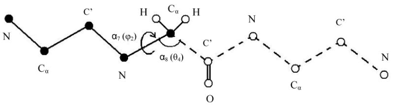
Illustration of the HSMC(D) reconstruction process of conformation i of a peptide consisting of three glycine residues. At each step the transition probability (TP) of a dihedral angle and the successive bond angle is determined and the related atoms are then fixed in their positions in i. The figure describes step 4 where the dihedral and bond angles considered are φ2 (of the second residue) and the successive θ; these coordinates are also denoted α7 and α8, respectively (see text). In this process the already reconstructed part (the past) is depicted with solid lines and solid spheres (atoms); for simplicity the oxygens and most of the hydrogens are discarded. The TP is obtained by carrying out an MD simulation of the as yet unreconstructed part of the peptide (the future) which is depicted with dashed lines and empty spheres. In this simulation the “past” atoms remain fixed at their positions in i while the conformations of the future part should remain within the limits of the microstate; future-past interactions are taken into account. Small bins δφ2 and δθ are centered at the values of φ2 and θ in i. The TP is calculated from the number of simultaneous visits of the future part to δφ2 and δθ during the simulation [see equation (23)]. After TP(4) has been determined the coordinates of the two hydrogen atoms of Cα (2) and those of C′(2) are fixed at their positions in i and the process continues.
| (23) |
Notice that in the deterministic calculation of Zfuture, [equation (19)] the limits of Ωh are in practice unknown. On the other hand, with HSMD the future structures generated by MD at each step k remain in general within the limits of the microstate Ωh defined by the analyzed MD sample due to the microstate's (meta) stability.
Similar to equation (20), the corresponding overall probability density for HSMD is
| (24) |
where in the product only odd values of k are used. ρHS(α6N,⋯,α1) defines an approximate entropy and free energy functionals, SA and FA (over the ensemble) which can be shown using Jensen's inequality to constitute rigorous upper and lower bounds, respectively [117],
| (25) |
| (26) |
In these equations ρHS = ρHS(α6N,⋯,α1), <E> is the Boltzmann average of the potential energy (force field), estimated from the MD sample and ρB [equation (20)] is the (correct) Boltzmann probability density with which the sample has been generated. SA is estimated from a Boltzmann sample of size n by the arithmetic average of the ln(ρHS) values [see equation (7)]. As discussed in II.1, the fluctuation (standard deviation), σF of the correct free energy [equation (5)] is zero, while the approximate FA has finite fluctuation, σA (estimated by its arithmetic average, ), which is expected to decrease as the approximation improves (i.e., as nf increases and/or δαk decreases) [13,14,115-117]
| (27) |
One can also define a free energy functional, FB which constitutes a rigorous upper bound for the correct F [116,117]. Thus, by increasing computer time (and/or decreasing δαk)) a set of improving bounds can be obtained which enable one to determine the accuracy from HSMC(D) results alone without the need to know the correct answer (a “self checking” property). Furthermore, F can be obtained from a very small sample and even from any single conformation (see discussion in II.1). A functional FD has been also been defined, which leads to the correct F, and additionally, the correct F can also be estimated from the anti-correlation between improving results of FA and its fluctuation, σA (FA increases where σA decreases). However, FB and FD are statistically less reliable than FA. These topics have been developed and tested in a systematic way in particular for argon, water, and self-avoiding walks on a lattice [116-118] (see below).
Unlike the limited applicability of methods that are based on harmonic approximations, HSMC(D) is applicable to fluids, random coil polymers, as well as microstates of a peptide. Thus, results for liquid argon, TIP3P water [117,125], and self-avoiding walks on a square lattice [118] were found to agree within error bars to TI results. Also, for polyglycine molecules, differences ΔFmn and ΔSmn for α-helix, extended, and hairpin microstates were calculated very reliably by HSMC [30]. However, in principle, HSMC(D) is not an efficient method because the number of build-up steps increases with system size. It turns out, however, that in calculations of differences ΔSmn = Sm−Sn (or ΔFmn) (that are of our main interest) the accuracy of and can be compromised significantly without degrading the accuracy of the calculated difference [e.g., by using small nf and/or a large bin, δαk; see equations (22) and (23)] due to cancellation of systematic errors. Thus, is equal to the correct value within the statistical errors, as has been demonstrated for peptides [29,30,32] as well as for the 7-residue mobile loop, 304-310 (Gly-His-Gly-Ala-Gly-Gly-Ser) of the enzyme porcine pancreatic α-amylase. This loop was modeled in vacuum by the AMBER force field, by AMBER with implicit solvation [120] and with explicit water [121]. Such cancellation of errors (discussed below) is typical of methods that calculate the absolute S (F) and it occurs especially for HSMD leading to a dramatic increase in its efficiency (see end of next section).
III.3.b.4 The cancellation of systematic errors with HSMD
It is important to understand the basis for the cancellation of errors discussed above. We examine first two one-dimensional harmonic microstates (oscillators) with the same mass defined by different spring constants f1 and f2. The exact entropy difference, ΔSmn (here written ΔS2,1 can be expressed in terms of the variances <x2> and <y2> of the corresponding coordinates,
| (28) |
One can estimate ΔS2,1 from two separate MD simulations, where the corresponding variances are calculated. If f1 is significantly smaller than f2 (i.e., f1 defines a flatter parabola) and the same step size is used in both simulations a longer simulation will be required for f1 than for f2 to gain the same statistical precision. Therefore, if the same sample size is used for both microstates the statistical precision of ΔS2,1 will be determined mostly by that of S1.
We now examine the entropy contributed by a backbone dihedral angle, αk (denoted α for simplicity) in the course of the reconstruction process. α varies in microstates 1 and 2 within the ranges Δα1 and Δα2 [equation (21)] which we denote Δ1 and Δ2, respectively. The crudest (but sometimes quite reliable) HSMD approximation for the corresponding difference in entropy ΔS0(α) is
| (29) |
which is similar to that of equation (28) above (for brevity we shall omit α from the equations below). For better HSMD approximations, we define the bins δ1=Δ1/l and δ2=Δ2/l, where l is an increasing integer; the corresponding probabilities are and which are defined by nvisit/nf [equations (22) and (23)]. One obtains,
| (30) |
where can be viewed as an an-harmonic term. One can write, for i=1,2, where and are thus factors (systematic errors) satisfying for very large nf; for a given l (bin) one obtains,
| (31) |
However, for large bins, δ (small l), one would expect to obtain probabilities that are close to the exact ones, and [i.e., and are ∼1] for a relatively small nf due to adequate statistics, i.e., relatively large nvisit values. To obtain the exact probabilities (within the statistical errors) for decreased bin sizes, nf should be increased adequately, which might increase computer time significantly. Thus, for practical values of nf, and might differ significantly from 1 (i.e., large systematic errors). However, we argue that already for relatively small nf, and the last logarithmic term [equation (31)] becomes smaller than the statistical error leading to the correct value, ΔS(l) within the statistical error. To obtain the correct contribution (ΔS) of dihedral angle α to the entropy difference one has to define small enough bins, i.e., large enough lmin, where for l>lmin ΔS(l) remains unchanged within the statistical error.
The relation stems from two reasons, where the first one is the fact that HSMD takes all interactions into account and thus for a given nf the future part of the chain is treated with the same level of approximation in both microstates. Secondly, because with MD the atoms are moved along their potential gradients, the simulations are equally efficient in both microstates. For peptides [32] the condition occurs for much smaller nf with HSMD than with HSMC [30] because the efficiency of the MC procedure used depends on the compactness of a structure (e.g., hairpin versus extended); correspondingly, the computer time required with HSMD was reduced by a factor of ∼100 as compared to that needed with HSMC. Again, as for the parabolas above, if one microstate is significantly “flatter” than the other (i.e., larger Δαk values), the required nf value for obtaining convergence of ΔS will be determined mainly by the flatter microstate.
III.3.b.5 The HS and LS methods
With the HS method one seeks to reconstruct a chain by a deterministic calculation of Zfuture [equation (19)] for each αk, based only on a partial future scanning defined by αk,αk+1…αk+f, where f is the scanning parameter, f«6N. HS works very well for self-avoiding walks on a lattice [14,112,115,118], argon [126], or magnetic models [114], because these systems are not limited to a microstate, i.e., the future scanning at each step is carried out over the entire (available) configurational space. On the other hand, for a peptide in a microstate, HS is practically not applicable, because of the difficulty to define the limits of the future part of a microstate in conformational space, as discussed in II.4.
With the LS method applied to a peptide, [22-28] the conformations of a given sample (of a microstate) are initially expressed in terms of internal coordinates and then a three-stage analysis is carried out where the sample is visited three times. In the first visit the variability range Δαk is calculated, [equation (21)]. Each range, Δαk is then divided into l equal segments, where l is the discretization parameter. We denote these segments by νk, (νk=1,l). Thus, an angle αk is now represented by the segment νk to which it belongs and a conformation i is expressed by the corresponding vector of segments [ν1(i), ν2(i), …, ν6N (i)]. Under this discretization approximation a set of TP densities, ρ(αk|αk−1,⋯,α1) can in principle be estimated by
| (32) |
where n(νk,⋯,ν1) is the number of times the local state [i.e., the partial vector (νk,⋯,ν1) representing (αk,⋯,α1)] appears in the sample. Because the number of local states increases exponentially with k one has to resort to approximations based on smaller local states that consists of νk and the b angles preceding it along the chain, i.e., the vector (νk,νk-1, …,νk-b), where b is the correlation parameter. The sample is visited for the second time and for a given b one calculates the number of occurrences n(νk,νk-1, …,νk-b) of all the local states from which a set of transition probabilities p(νk| νk-1,…, νk-b) are defined. The sample is then visited for the third time and for each member i of the sample one determines the 6N local states and the corresponding transition probabilities, whose product defines an approximate probability density ρi(b,l) for conformation i
| (33) |
the larger are b and l the better the approximation (for enough statistics). ρi(b,l) allows one to define an approximate entropy and free energy functionals, SA and FA=<E>-TSA [as in equations (25) and (26), where ρi(b,l) replaces ρHS(α6N,⋯,α1)], which constitute rigorous upper and lower bounds for the correct values, respectively [22]. Thus, with LS, the past is treated approximately where the entire future is taken into account, in contrast to HS where the whole past is considered but only part of the future is taken into account. To improve the approximation of these methods, the parameters (b,l) and f should be increased, which requires, respectively, very large samples with LS (to get the adequate statistics), and a lot of computer time for calculating Zf(HS). LS has been applied very successfully to peptides [22-25,27,28], loops [26] as well as magnetic lattice systems, lattice gas models [111,114] and fluid dynamics [127]. However, for random coil polymers (self-avoiding walks) LS is much less efficient than HS [115].
The above discussion demonstrates that LS (unlike HS) is of a “geometrical” character, i.e., calculation of the entropy does not depend directly on the interaction energy. Other methods that are based on calculating the distribution of local states (but not transition probabilities) have been suggested recently by Hnizdo et al. [128] and Killian et al. [129] who tested them on small molecules and peptides.
Finally, it should be pointed out that both LS, the above two methods, and the mining minima technique [99,100] can be applied to samples based on several microstates (where LS is also applicable to the random coil state), while QH lead to reliable results only for a single microstate [105]. However, QH, which considers the (quadratic) correlations among all variables, is expected to lead to better results than LS for a single microstate. Indeed, for peptides [30,32] and a surface loop of the protein α-amylase [120,121] the entropy results of QH were found to be better (i.e., smaller) than those of LS based on b=2 and l=10. However, the corresponding results for S[HSMC(D)] have always been the lowest (i.e., better).
III.3.b.6 Calculation of differences Sm - Sn
With QH, LS, and HSMC(D) calculation of ΔSmn=Sm–Sn is based on the absolute values for each microstate. However, in section II.4 we have argued that the definition of a microstate m depends to a large extent on the simulation time t where typically m and its energy and entropy all grow with t. To be able to carry out a reliable estimation of ΔSmn (ΔFmn, etc.) we simulate both m and n for the same t looking for a range of t values where ΔFmn(t), ΔSmn(t) and ΔEmn(t) are stable within the statistical errors [due to simultaneous increase of Em(t), En(t), etc.]. For the QH method [equation (17)] such stable results constitute the best final answer. For the LS method, on the other hand, one can calculate [and ] for a set of improved approximations (by increasing b and l); if these differences converge within the statistical errors, the converged values are considered to be the correct differences due to cancellation of equal systematic errors in and (see III.3.b.4); this discussion also applies to different approximations of HSMC(D).
Obviously, if m is less stable than n the t values should be adjusted (i.e., decreased) to fit the stability of m. If m is significantly larger than n, tm should be large enough to allow an adequate coverage of m, tm ∼ tn[ΠΔαk(m)/[ΠΔαk(n)], where tn is the time required to obtain an adequate sample for n. However, if ΔSmn(t) increases monotonically it constitutes a lower bound. If the microstate is restrictive, e.g., side chains should populate a single rotamer, the MD sample can be composed of several smaller samples that each starts from the same structure (seed) with a different set of velocities. It should be pointed out that with LS and QH relatively large samples are required for obtaining converged TPs [24] and converged terms of the correlation matrix σ [equation (17)] [100], respectively. Therefore, one should verify that the samples remain in the original microstates and have not “escaped” to neighboring ones. For that, methods have been developed which enable one to analyze the stability of a microstate by calculating distribution profiles of dihedral angles [25,27,28].
Unlike QH and LS, HSMC(D) is not based on gathering statistics from the studied sample; therefore, the required sample size is relatively small; also, F[HSMC(D)] (but not necessarily E and S[HSMC(D)]) can be obtained from a very small sample (even from a single conformation) [117]. Therefore, in our studies of peptides and loops populating significantly different microstates [29,32,120,121] the sample size for HSMC(D) is small and has been determined by the range of t values for which the average of Em (En) is approximately constant (typically ∼600 conformations representing a 0.5 ns trajectory). Again, one can envisage extreme cases where m is significantly larger than n, which would require increasing the sample size for m as described above. In particular, with HSMC(D) the effect of sample size on ΔSmn=Sm-Sn can be reduced, while controlling this effect with TI and the counting approaches is difficult.
III.3.b.7 Calculation of the absolute F by TI
As pointed out earlier, the absolute S (F) can be obtained in principle also by TI, provided that a convenient reference state with known F is defined. In the early work of Stoessel and Nowak [130] a harmonic reference state UH=kΣ(ri-ri0)2 is defined, where k is a spring constant and ri and ri0 are the instantaneous and equilibrium coordinates of atom i, respectively. The hybrid Hamiltonian (H) depends on UH and the force field U, H(λ)=(1- λ)U + λUH (0 ≤ λ ≤ 1). For decaglycine in an α-helical microstate the estimated error in F (∼2 kcal/mole) is relatively high. Very recently [131], a similar idea has been implemented somewhat differently where H(λ) = U + (1/2)λUH and the free energy of the final state (λ=1) is calculated by a normal mode analysis. For the pentapeptide Met-enkephalin the maximum error in the absolute F of a microstate is again relatively high, ±1.5 kcal/mol (using HSMC(D), errors of ∼0.2 kcal/mol were obtained for ΔS (ΔF) between microstates of decaglycine and NH2(Val)2(Gly)6(Val)2CONH2 [30,32]).
In a recent paper [132] Ytreberg and Zuckerman define a simple numerically calculable reference state designed to overlap the particular microstate of interest. Here, the microstate (say, an α-helical state of a peptide) is first simulated locally by MD, where the range of each internal coordinate, k, is divided into bins, and (normalized) populations are obtained from the (MD) sample. Using these probabilities a large sample of reference system structures, i, is then generated with known probabilities, , where pk(i) is the probability of the bin of the kth internal coordinate in structure i. (Compare with the LS method above.) Each reference structure is assigned an energy defined by (which leads to Fref=0), and thus the desired free energy of the microstate can then be obtained through a standard perturbation expression, , where Ei is the actual force field energy calculated for the same set of coordinates (i). The method was found to work well for the leucine dipeptide; however, for a large microstate the overlap between the reference and real microstates might be small and therefore some enhancements should still be introduced.
III.3.b.8 methods based on Bennett's formula
Expressions for ΔFmn based on two separate simulations of m and n had been suggested by Bennett [75], where one of them was developed further by Voter [133]. Thus, a local MC simulation of microstate m (the sample is defined by vectors Rm) will not cover a distant microstate n (with Rn) as required by Bennett's expression that depends on both potential energies as Un-Um. Therefore, for a simulation of microstate m, a vector D leading from Rm to Rn is defined and the energy difference is obtained by Un(Rm+D)-Um(Rm), and similarly Um(Rn-D)-Un(Rn) for a simulation of microstate n. Specifically
| (34) |
where MT is the Metropolis function, MT(ΔE)=min[1,exp(ΔE/kBT)] and <>n and <>m denote averages over m and n, respectively. These ideas have been investigated recently further by Ytreberg and Zuckerman [134] who calculated free energy and entropy differences between microstates of peptides described by internal coordinates using a “single state shifting protocol”. However, the results depend on the number (and type) of shifted coordinates, for which no selection criterion has been provided.
Finally, we provide a short list of other recent methods for calculating F (S). Two methods involve TI [135,136] and one is based on the identity 1/Q=<w(p,x)exp[H(p,x)/kBT]>, where Q is the partition function, p is the momentum and w(p,x) is a weight function [137]; this identity is used in HSMC(D) [117] and was used before with various w functions. With another method the joint probability density is represented by a two-dimensional Fourier series [138], and in a fourth method energy decomposition approach is used for evaluating S [139]. We mention also two methods for calculating the absolute protein-ligand binding free energy [140,141] and a method for calculating free energy profiles of enzymatic reactions by the linear response approximation [142].
IV. Conclusions
In this review we have discussed the difficulties in calculating the entropy S and the free energy F focusing on the related problems involved in the definition and simulation of microstates of peptides and proteins. While the review is broad, the emphasis is on efficiency issues related to recently developed techniques, in particular techniques for calculating the absolute F (S), where our HSMC(D) method is discussed in some detail. We describe equilibrium and non-equilibrium techniques for calculating the relative binding free energy of ligands to an active site; however, methods for calculating the standard absolute binding free energy have not been covered. Also, we do not elaborate on practical aspects of protein-ligand (DNA-ligand, etc.) interactions, such as modeling of the solvent and calculating its contribution to the free energy. These topics are dealt more extensively in other recent reviews [8,9].
In this context one should emphasize the strong effects of modeling (in particular of electrostatic interactions) on the results for F (S) and other thermodynamic and structural properties. In fact, incompatibility of theoretical results with experimental data due to unreliable modeling can be much more severe than method-related inaccuracies in the calculation of F (S). Therefore, to gain progress in computational structural biology, the existing force fields and solvation models should be improved, efficient techniques for simulation of biological macromolecules should be devised, as well as better techniques for calculating F (S).
TI is the most general methodology, which in many cases is also the easiest to implement. Furthermore, various versions of TI (in particular procedures for calculating the relative free energy of ligands bound to an active site) are already programmed in the commonly used molecular mechanics/molecular dynamics software packages (see II.2.a). Among the TI based techniques, AIM [63,93] appears to be very efficient (at least for the systems studied), but it has not been applied as yet to biological molecules. Simulation methods (e.g., the multicanonical method) that lead to an efficient conformational search and based (like AIM) on an adaptive buildup of the (relative) free energy, have been applied to small biological macromolecules - peptides and loops (see II.2.b); these simulations have been performed with in-house programs. Also, path-based limitations in TI have led to the development of techniques for computing the absolute F (S). Thus, calculation of ΔFmn=Fm-Fn, which avoids the need to carry out reversible (or non-reversible) thermodynamic integration, has clear advantages, as discussed earlier. However, for an N-atom system the fluctuation in Sm (and practically also in an approximate Fm) is ∼N1/2 and for large N estimating small ΔFmn values would be unfeasible. Also, most methods for calculating the absolute Fm (Sm) discussed here are not applicable (at least as yet) to diffusive systems (e.g., water) and further developments in this direction are needed. Moreover, many methods do not provide criteria for estimating their accuracy; the QH method, which belongs to this category, should be used with caution [105]. In this respect HSMC(D) [29-32,116-119,120,121] (which still needs further development) has clear advantages: it is applicable to diffusive systems and to any chain flexibility (microstates as well as the random coil state), and it provides self-checking means for estimating its accuracy. Programming of QH, LS, and other techniques in this category (e.g., Bennett's procedure) is relatively easy and is usually carried out in-house. HSMC(D) is being developed within the framework of TINKER [62] and the software will become available when completed.
Acknowledgments
We thank Dan Zuckerman, Marty Ytreberg, and Mihail Mihailescu for valuable discussions. This work was partially supported by National Science Foundation Information Technology Research Grant, NSF 0225636 and NIH grant 2 R01 GM066090-04 A2.
Abbreviations
- MC
Monte Carlo
- MD
Molecular dynamics
- HS
Hypothetical scanning method
- HSMC(D)
Hypothetical scanning MC (MD) method
- LS
Local states method
- AIM
Adaptive integration method
- TI
Thermodynamic integration
- FEP
Free energy perturbation
References
- 1.Beveridge DL, DiCapua FM. Free energy via molecular simulation: applications to chemical and biomolecular systems. Annu Rev Biophys Biophys Chem. 1989;18:431–492. doi: 10.1146/annurev.bb.18.060189.002243. [DOI] [PubMed] [Google Scholar]
- 2.Kollman PA. Free energy calculations: applications to chemical and biochemical phenomena. Chem Rev. 1993;93:2395–2417. [Google Scholar]
- 3.Jorgensen WL. Free energy calculations: a breakthrough for modeling organic chemistry in solution. Acc Chem Res. 1989;22:184–189. [Google Scholar]
- 4.Meirovitch H. Calculation of the free energy and entropy of macromolecular systems by computer simulation. In: Lipkowitz KB, Boyd DB, editors. Reviews in Computational Chemistry. Vol. 12. Wiley-VCH; New York: 1998. pp. 1–74. [Google Scholar]
- 5.Gilson MK, Given JA, Bush BL, McCammon JA. The statistical thermodynamic basis for computing of binding affinities: A critical review. Biophys J. 1997;72:1047–1069. doi: 10.1016/S0006-3495(97)78756-3. [DOI] [PMC free article] [PubMed] [Google Scholar]
- 6.Boresch S, Tttinger F, eitgeb M, Karplus M. Absolute binding free energies: A qualitative approach for their calculation. J Phys Chem B. 2003;107:9535–9551. [Google Scholar]
- 7.Meirovitch H. Recent developments in methodologies for calculating entropy and free energy of biological systems by computer simulation. Curr Opinion in Struct Biol. 2007;17:181–186. doi: 10.1016/j.sbi.2007.03.016. [DOI] [PubMed] [Google Scholar]
- 8.Gilson MK, Zhou HX. Calculation of protein-ligand binding affinities. Ann Rev Biophys Biomol Struct. 2007;36:21–42. doi: 10.1146/annurev.biophys.36.040306.132550. [DOI] [PubMed] [Google Scholar]
- 9.Foloppe N, Hubbard R. Towards predictive ligand design with free-energy based Computational methods? Curr Med Chemistry. 2007;13:3583–3608. doi: 10.2174/092986706779026165. [DOI] [PubMed] [Google Scholar]
- 10.Metropolis N, Rosenbluth AW, Rosenbluth MN, Teller AH, Teller E. Equation of state calculations by fast computing machines. J Chem Phys. 1953;21:1087–1092. [Google Scholar]
- 11.Alder BJ, Wainwright TE. Studies of molecular dynamics. I. General method. J Chem Phys. 1959;31:459–466. [Google Scholar]
- 12.McCammon JA, Gelin BR, Karplus M. Dynamics of folded proteins. Nature. 1977;267:585–590. doi: 10.1038/267585a0. [DOI] [PubMed] [Google Scholar]
- 13.Meirovitch H, Alexandrowicz Z. On the zero fluctuation of the microscopic free energy and its potential use. J Stat Phys. 1976;15:123–127. [Google Scholar]
- 14.Meirovitch H. Simulation of a free energy upper bound, based on the anti-correlation between an approximate free energy functional and its fluctuation. J Chem Phys. 1999;111:7215–7224. [Google Scholar]
- 15.Elber R, Karplus M. Multiple conformational states of proteins - a molecular dynamics analysis of myoglobin. Science. 1987;235:318–321. doi: 10.1126/science.3798113. [DOI] [PubMed] [Google Scholar]
- 16.Stillinger FH, Weber TA. Packing structures and transitions in liquids and solids. Science. 1984;225:983–989. doi: 10.1126/science.225.4666.983. [DOI] [PubMed] [Google Scholar]
- 17.Getzoff ED, Geysen HM, Rodda SJ, Alexander H, Tainer JA, Lerner RA. Mechanisms of antibody binding to a protein. Science. 1987;235:1191–1196. doi: 10.1126/science.3823879. [DOI] [PubMed] [Google Scholar]
- 18.Rini JM, Schulze-Gahmen U, Wilson IA. Structural evidence for induced fit as a mechanism for antibody- antigen recognition. Science. 1992;255:959–965. doi: 10.1126/science.1546293. [DOI] [PubMed] [Google Scholar]
- 19.Constantine KL, Friedrichs MS, Wittekind M, Jamil H, Chu CH, Parker RA, Goldfarb V, Mueller L, Farmer BT. Backbone and side chain dynamics of uncomplexed human adipocyte and muscle fatty acid-binding proteins. Biochemistry. 1998;37:7965–7980. doi: 10.1021/bi980203o. [DOI] [PubMed] [Google Scholar]
- 20.Korzhnev DM, Salvatella X, Vendruscolo M, Di Nardo AA, Davidson AR, Dobson CM, Kay LE. Low populated folding intermediates of Fyn SH3 characterized by relaxation dispersion NMR. Nature. 2004;430:586–590. [Google Scholar]
- 21.Eisenmesser EZ, Millet O, Labeikovski W, Korzhnev DM, Wolf-Watz M, Bosco DA, Skalicky JJ, Kay LE, Kern D. Intrinsic dynamics of an enzyme underlies catalysis. Nature. 2005;438:117–121. doi: 10.1038/nature04105. [DOI] [PubMed] [Google Scholar]
- 22.Meirovitch H, Vásquez M, Scheraga HA. Stability of polypeptides conformational states as determined by computer simulation of the free energy. Biopolymers. 1987;26:651–671. doi: 10.1002/bip.360260508. [DOI] [PubMed] [Google Scholar]
- 23.Meirovitch H, Kitson DH, Hagler AT. Computer simulation of the entropy of polypeptides using the local states method: Application to Cyclo-(Ala-Pro-D-Phe)2 in vacuum and the crystal. J Am Chem Soc. 1992;114:5386–5399. [Google Scholar]
- 24.Meirovitch H, Koerber SC, Rivier J, Hagler AT. Computer simulation of the free energy of peptides with the local states method: Analogues of gonadotropin releasing hormone in the random coil and stable states. Biopolymers. 1994;34:815–839. doi: 10.1002/bip.360340703. [DOI] [PubMed] [Google Scholar]
- 25.Meirovitch H, Meirovitch E. New theoretical methodology for elucidating the solution structure of peptides from NMR data. III. Solvation effects. J Phys Chem. 1996;100:5123–5133. doi: 10.1002/(sici)1097-0282(199601)38:1<69::aid-bip6>3.0.co;2-u. [DOI] [PubMed] [Google Scholar]
- 26.Meirovitch H, Hendrickson TF. The backbone entropy of loops as a measure of their flexibility. Application to a ras protein simulated by molecular dynamics. Proteins. 1997;29:127–140. [PubMed] [Google Scholar]
- 27.Baysal C, Meirovitch H. Free energy based populations of interconverting microstates of a cyclic peptide lead to the experimental NMR data. Biopolymers. 1999;50:329–344. doi: 10.1002/(SICI)1097-0282(199909)50:3<329::AID-BIP8>3.0.CO;2-4. [DOI] [PubMed] [Google Scholar]
- 28.Baysal C, Meirovitch H. Ab initio structure prediction of a cyclic pentapeptide in DMSO based on an implicit solvation model. Biopolymers. 2000;53:423–433. doi: 10.1002/(SICI)1097-0282(20000415)53:5<423::AID-BIP6>3.0.CO;2-C. [DOI] [PubMed] [Google Scholar]
- 29.Cheluvaraja S, Meirovitch H. Simulation method for calculating the entropy and free energy of peptides and proteins. Proc Natl Acad Sci USA. 2004;101:9241–9246. doi: 10.1073/pnas.0308201101. [DOI] [PMC free article] [PubMed] [Google Scholar]
- 30.Cheluvaraja S, Meirovitch H. Calculation of the entropy and free energy by the hypothetical scanning Monte Carlo Method: Application to peptides. J Chem Phys. 2005;122:054903–14. doi: 10.1063/1.1835911. [DOI] [PubMed] [Google Scholar]
- 31.Cheluvaraja S, Meirovitch H. Calculation of the entropy and free energy from Monte Carlo simulations of a peptide stretched by an external force. J Phys Chem B. 2005;109:21963–21970. doi: 10.1021/jp052969l. [DOI] [PMC free article] [PubMed] [Google Scholar]
- 32.Cheluvaraja S, Meirovitch H. Calculation of the entropy and free energy of peptides by molecular dynamics simulations using the hypothetical scanning molecular dynamics method. J Chem Phys. 2006;125:024905–13. doi: 10.1063/1.2208608. [DOI] [PubMed] [Google Scholar]
- 33.Garcia AE, Sanbonmatsu KY. Exploring the energy landscape of a beta hairpin in explicit solvent. Proteins. 2001;42:345–354. doi: 10.1002/1097-0134(20010215)42:3<345::aid-prot50>3.0.co;2-h. [DOI] [PubMed] [Google Scholar]
- 34.Berg BA, Neuhaus T. Multicanonical algorithms for first order phase transition. Phys Lett B. 1991;267:249–253. doi: 10.1103/PhysRevLett.68.9. [DOI] [PubMed] [Google Scholar]
- 35.Ikeda K, Galzitskaya OV, Nakamura H, Higo J. β-hairpins, a-helices, and the intermediates among the secondary structures in the energy landscape of a peptide from a distal β-hairpin of SH3 domain. J Comput Chem. 2003;24:310–318. doi: 10.1002/jcc.10160. [DOI] [PubMed] [Google Scholar]
- 36.Nguyen PH, Stock G, Mittag E, Hu CK, Li MS. Free energy landscape and fold mechanism of a β-hairpin in explicit water: a replica exchange molecular dynamics study. Proteins. 2005;61:795–808. doi: 10.1002/prot.20696. [DOI] [PubMed] [Google Scholar]
- 37.Lange OF, Grubmüller H. Collective Langevin dynamics of conformational motions in proteins. J Chem Phys. 2006;124:214903–18. doi: 10.1063/1.2199530. [DOI] [PubMed] [Google Scholar]
- 38.MacDonald IR, Singer K. Machine calculation of thermodynamic properties of a simple fluid. J Chem Phys. 1967;47:4766–4772. [Google Scholar]
- 39.Hansen JP, Verlet L. Phase transition of the Lennard –Jones system. Phys Rev. 1969;184:151–161. [Google Scholar]
- 40.Hoover WG, Ree FH. Use of computer experiments to locate the melting transition and calculate the entropy in the solid phase. J Chem Phys. 1967;47:4873–4878. [Google Scholar]
- 41.Allen MP, Tildesley DJ. Computer Simulation of Liquids. Clarenden Press; Oxford: 1987. [Google Scholar]
- 42.Kirkwood JG. Statistical mechanics of fluid mixtures. J Chem Phys. 1935;3:300–313. [Google Scholar]
- 43.Zwanzig RW. High-temperature equation of state by a perturbation method. I. Nonpolar gases. J Chem Phys. 1954;22:1420–1426. [Google Scholar]
- 44.Squire DR, Hoover WG. Monte Carlo simulation of vacancies in rare-gas crystals. J Chem Phys. 1969;50:701–706. [Google Scholar]
- 45.Torrie GM, Valleau JP. Monte Carlo free energy estimates using non-Boltzmann sampling. Application to the subcritical Lennard-Jones fluid. Chem Phys Lett. 1974;28:578–581. [Google Scholar]
- 46.Torrie GM, Valleau JP. Nonphysical sampling distributions in Monte Carlo free energy estimation: Umbrella sampling. J Comp Phys. 1977;23:187–199. [Google Scholar]
- 47.Jarzynski C. Nonequilibrium equality for free energy differences. Phys Rev Lett. 1997;78:2690–2693. [Google Scholar]
- 48.Ferrenberg AM, Swendsen RH. Optimized Monte Carlo data analysis. Phys Rev Lett. 1989;63:1195–1198. doi: 10.1103/PhysRevLett.63.1195. [DOI] [PubMed] [Google Scholar]
- 49.Kumar S, Rosenberg JM, Bouzida D, Swendsen RH, Kolmann PA. Multidimensional free energy calculations using the weighted histogram analysis method. J Comput Chem. 1995;16:1339–1350. [Google Scholar]
- 50.Kumar S, Payne PW, Vásquez M. Method for free energy calculations using iterative technique. J Comput Chem. 1996;17:1269–1275. [Google Scholar]
- 51.Fleischman SH, Brooks CL., III Thermodynamics of aqueous solvation: Solution properties of alcohols and alkanes. J Chem Phys. 1987;87:3029–3037. [Google Scholar]
- 52.Peter C, Oostenbrink C, van Dorp A, van Gunsteren WF. Estimating entropies from molecular dynamics simulations. J Chem Phys. 2004;120:2652–2661. doi: 10.1063/1.1636153. [DOI] [PubMed] [Google Scholar]
- 53.Wan S, Stote RH, Karplus M. Calculation of the aqueous solvation energy and entropy, as well as free energy of simple polar solutes. J Chem Phys. 2004;121:9539–9548. doi: 10.1063/1.1789935. [DOI] [PubMed] [Google Scholar]
- 54.Miyamoto S, Kollman PA. Absolute and relative binding free energy calculations of the interaction of biotin and its analogs with streptavidin using molecular dynamics/free energy perturbation approaches. Proteins. 1993;16:226–245. doi: 10.1002/prot.340160303. [DOI] [PubMed] [Google Scholar]
- 55.Miyamoto S, Kollman PA. What determines the strength of noncovalent association of ligands to proteins in aqueous solution. Proc Natl Acad Sci USA. 1993;90:8402–8406. doi: 10.1073/pnas.90.18.8402. [DOI] [PMC free article] [PubMed] [Google Scholar]
- 56.Cornell WD, Cieplak P, Bayly CI, Gould IR, Merz KM, Jr, Ferguson DM, Spellmeyer DC, Fox T, Caldwell JW, Kollman PA. A second generation force field for the simulation of proteins,nucleic acids, and organic molecules. J Am Chem Soc. 1995;117:5179–5197. [Google Scholar]
- 57.MacKerell AD, Jr, Bashford D, Bellott M, Dunbrack RL, Jr, Evanseck JD, Field MJ, Fischer S, Gao J, Guo H, Ha S, Joseph-McCarthy D, Kuchnir L, Kuczera K, Lau FTK, Mattos C, Michnick S, Ngo T, Nguyen DT, Prodhom B, Reiher WE, III, Roux B, Schlenkrich M, Smith JC, Stote R, Straub J, Watanabe M, Wiórkiewicz-Kuczera J, Yin D, Karplus M. All-atom empirical potential for molecular modeling and dynamics studies of proteins. J Phys Chem B. 1998;102:3586–3616. doi: 10.1021/jp973084f. [DOI] [PubMed] [Google Scholar]
- 58.Phillips JC, Braun R, Wang W, Gumbart J, Tajkhorshid E, Villa E, Chipot C, Skeel RD, Kalé L, Schulten K. Scalable molecular dynamics with NAMD. J Comput Chem. 2005;26:1781–1802. doi: 10.1002/jcc.20289. [DOI] [PMC free article] [PubMed] [Google Scholar]
- 59.Jorgensen WL, Tirado-Rives J. Molecular modeling of organic and biomolecular systems using BOSS and MCPRO. J Comput Chem. 2005;26:1689–1700. doi: 10.1002/jcc.20297. [DOI] [PubMed] [Google Scholar]
- 60.Christen M, Hünenberger PH, Bakowies D, Baron R, Bürgi R, Geerke DP, Heinz TN, Kastenholz MA, Kraütler V, Oostenbrink C, Peter C, Trzesniak D, Van Gunsteren WF. The GROMOS software for biomolecular simulation: GROMOS05. J Comput Chem. 2005;26:1719–1751. doi: 10.1002/jcc.20303. [DOI] [PubMed] [Google Scholar]
- 61.Van Der Spoel D, Lindahl E, Hess B, Groenhof G, Mark AE, Berendsen HJC. GROMACS: Fast, flexible, and free. J Comput Chem. 2005;26:1701–1718. doi: 10.1002/jcc.20291. [DOI] [PubMed] [Google Scholar]
- 62.Ponder JW. TINKER - software tools for molecular design, version 4.2. 2004 doi: 10.1021/acs.jctc.8b00529. [DOI] [PMC free article] [PubMed] [Google Scholar]
- 63.Fasnacht M, Swendsen RH, Rosenberg JM. Adaptive integration method for Monte Carlo simulations. Phys Rev E. 2004;69:056704–15. doi: 10.1103/PhysRevE.69.056704. [DOI] [PubMed] [Google Scholar]
- 64.Lyubartsev AP, Martsinovski AA, Shevkunov SV, Vorontsov-Velyaminov PN. New approach to Monte Carlo calculation of the free energy: Method of expanded ensembles. J Chem Phys. 1992;96:1776–1783. [Google Scholar]
- 65.Marinari E, Parisi G. Simulated Tempering: a New Monte Carlo Scheme. Europhys Lett. 1992;19:451–455. [Google Scholar]
- 66.Wang F, Landau DP. Efficient multiple-range random walk algorithm to calculate the density of states. Phys Rev Lett. 2001;86:2050–2053. doi: 10.1103/PhysRevLett.86.2050. [DOI] [PubMed] [Google Scholar]
- 67.Rathore N, Knotts TA, III, de Pablo JJ. Density of states simulations of proteins. J Chem Phys. 2003;118:4285–4290. doi: 10.1016/S0006-3495(03)74810-3. [DOI] [PMC free article] [PubMed] [Google Scholar]
- 68.Mastny EA, de Pablo JJ. Direct calculation of solid-liquid equilibria from density of states Monte Carlo simulations. J Chem Phys. 2005;122:124109–6. doi: 10.1063/1.1874792. [DOI] [PubMed] [Google Scholar]
- 69.Chopra M, Müller M, de Pablo JJ. Order-parameter-based Monte Carlo simulation of crystallization. J Chem Phys. 2006;124:134102–8. doi: 10.1063/1.2178324. [DOI] [PubMed] [Google Scholar]
- 70.Fenwick MK, Escobedo FA. Expanded ensemble and replica exchange methods for simulation of protein-like systems. J Chem Phys. 2003;119:11998–12010. [Google Scholar]
- 71.Fenwick MK, Escobedo FA. On the use of Bennett's acceptance ratio method in multi-canonical-type simulations. J Chem Phys. 2004;120:3066–3074. doi: 10.1063/1.1641000. [DOI] [PubMed] [Google Scholar]
- 72.Gospodinov ID, Escobedo FA. Multicanonical schemes for mapping out free energy landscapes of single-component and multicomponent systems. J Chem Phys. 2005;122:164103–10. doi: 10.1063/1.1884594. [DOI] [PubMed] [Google Scholar]
- 73.Abreu CRA, Escobedo FA. A general framework for non-Boltzmann Monte Carlo sampling. J Chem Phys. 2006;124:054116–12. doi: 10.1063/1.2165188. [DOI] [PubMed] [Google Scholar]
- 74.Escobedo FA. Optimized expanded ensembles for simulations involving molecular insertions and deletions. II. Open systems. J Chem Phys. 2007;127:174104–12. doi: 10.1063/1.2800321. [DOI] [PubMed] [Google Scholar]
- 75.Bennett CH. Efficient estimation of free energy differences from Monte Carlo data. J Comput Phys. 1976;22:245–268. [Google Scholar]
- 76.Mitsutake A, Sugita Y, Okamoto Y. Replica-exchange multicanonical and multicanonical replica-exchange Monte Carlo simulations of peptides. II. Application to a more complex system. J Chem Phys. 2003;118:6676–6688. [Google Scholar]
- 77.Sugita Y, Okamoto Y. Molecular mechanism for stabilizing a short helical peptide studied by generalized-ensemble simulations with explicit solvent. Biophys J. 2005;88:3180–3190. doi: 10.1529/biophysj.104.049429. [DOI] [PMC free article] [PubMed] [Google Scholar]
- 78.Yoda T, Sugita Y, Okamoto Y. Cooperative folding mechanism of a β-hairpin peptide studied by a multicanonical replica-exchange molecular dynamics simulation. Proteins. 2007;66:846–859. doi: 10.1002/prot.21264. [DOI] [PubMed] [Google Scholar]
- 79.Nakajima N, Nakamura H, Kidera A. Multicanonical ensemble generated by molecular dynamics simulation for enhanced sampling of peptides. J Phys Chem B. 1997;101:817–824. [Google Scholar]
- 80.Fukunishi Y, Mikami Y, Nakamura H. The filling potential method: A method for estimating the free energy surface for protein-ligand docking. J Phys Chem B. 2003;107:13201–13210. [Google Scholar]
- 81.Watanabe YS, Kim JG, Fukunishi Y, Nakamura H. Free energy landscapes of small peptides in an implicit solvent model determined by force-biased multicanonical molecular dynamics simulation. Chem Phys Lett. 2004;400:258–263. [Google Scholar]
- 82.Kamiya N, Yonezawa Y, Nakamura H, Higo J. Protein-inhibitor flexible docking by a multicanonical sampling: Native complex structure with the lowest free energy and a free-energy barrier distinguishing the native complex from the others. Proteins. 2008;70:41–53. doi: 10.1002/prot.21409. [DOI] [PubMed] [Google Scholar]
- 83.Ytreberg FM, Zuckerman DM. Efficient use of nonequilibrium measurement to estimate free energy differences for molecular systems. J Comput Chem. 2004;25:1749–1759. doi: 10.1002/jcc.20103. [DOI] [PubMed] [Google Scholar]
- 84.Ytreberg FM, Zuckerman DM. Single-ensemble nonequilibrium path-sampling estimates of free energy differences. J Chem Phys. 2004;120:10876–10879. doi: 10.1063/1.1760511. [DOI] [PubMed] [Google Scholar]
- 85.Jarzynski C. Rare events and convergence of exponentially averaged work values. Phys Rev E. 2006;73:046105–10. doi: 10.1103/PhysRevE.73.046105. [DOI] [PubMed] [Google Scholar]
- 86.Wu D, Kofke DA. Rosenbluth-sampled nonequilibrium work method for Calculation of free energies in molecular simulation. J Chem Phys. 2005;122:204104–13. doi: 10.1063/1.1906209. [DOI] [PubMed] [Google Scholar]
- 87.Oberhofer H, Dellago C, Geissler P. Biased sampling of nonequilibrium trajectories: can fast switching simulations outperform conventional free energy calculations methods? J Phys Chem. 2005;109:6902–6915. doi: 10.1021/jp044556a. [DOI] [PubMed] [Google Scholar]
- 88.Lechner W, Oberhofer H, Dellago C, Geissler P. Equilibrium free energies from fast-switching trajectories with large time step. J Chem Phys. 2006;124:044113–12. doi: 10.1063/1.2162874. 2006. [DOI] [PubMed] [Google Scholar]
- 89.MacFadyen J, Andricioaei I. A skewed-momenta method to efficiently generate conformational-transition trajectories. J Chem Phys. 2005;123:074107–9. doi: 10.1063/1.2000242. [DOI] [PubMed] [Google Scholar]
- 90.Adib AB. Free energy surfaces from nonequilibrium processes without work measurement. J Chem Phys. 2006;124:144111–5. doi: 10.1063/1.2188946. [DOI] [PubMed] [Google Scholar]
- 91.Shirts MR, Pande VS. Comparison of efficiency and bias of free energies computed by exponential averaging, the Bennett acceptance ratio, and thermodynamics integration. J Chem Phys. 2005;122:144107–16. doi: 10.1063/1.1873592. [DOI] [PubMed] [Google Scholar]
- 92.Jayachandran G, Shirts MR, Park S, Pande VJ. Parallelized-over-parts computation of absolute binding free energy with docking and molecular dynamics. J Chem Phys. 2006;125:084901–12. doi: 10.1063/1.2221680. [DOI] [PubMed] [Google Scholar]
- 93.Ytreberg FM, Swendsen RH, Zuckerman DM. Comparison of free energy methods for molecular simulations. J Chem Phys. 2006;125:184114–11. doi: 10.1063/1.2378907. [DOI] [PubMed] [Google Scholar]
- 94.Zhang D, Gullingsrud J, McCammon JA. Potential of mean force for a acetylcholine unbinding from the alpha7 nicotinic acetylcholine receptor ligand-binding domain. J Am Chem Soc. 2006;128:3019–3026. doi: 10.1021/ja057292u. [DOI] [PMC free article] [PubMed] [Google Scholar]
- 95.Xiong H, Crespo A, Marti M, Estrin D, Roitberg AE. Free energy calculations with non-equilibrium methods: applications of the Jarzynski relationship. Theor Chem Acc. 2006;116:338–346. [Google Scholar]
- 96.Gō N, Scheraga HA. Analysis of the contribution of internal vibrations to the statistical weights of equilibrium conformations of macromolecules. J Chem Phys. 1969;51:4751–4767. [Google Scholar]
- 97.Gō N, Scheraga HA. On the use of classical statistical mechanics in the treatment of polymer chain conformation. Macromolecules. 1976;9:535–542. [Google Scholar]
- 98.Hagler AT, Stern PS, Sharon R, Becker JM, Naider F. Computer simulation of the conformational properties of oligopeptides. Comparison of theoretical methods and analysis of experimental results. J Am Chem Soc. 1979;101:6842–6852. [Google Scholar]
- 99.Chang CE, Gilson MK. Tork: Conformational analysis method for molecules and complexes. J Comput Chem. 2003;24:1987–1998. doi: 10.1002/jcc.10325. [DOI] [PubMed] [Google Scholar]
- 100.Chen W, Chang CE, Gilson MK. Concepts in receptor optimization: targeting the RGD peptide. J Am Chem Soc. 2005;128:4675–4684. doi: 10.1021/ja056600l. [DOI] [PubMed] [Google Scholar]
- 101.Karplus M, Kushick JN. Method for estimating the configurational entropy of macromolecules. Macromolecules. 1981;14:325–332. [Google Scholar]
- 102.Rojas OL, Levy RM, Szabo A. Corrections to the quasiharmonic approximation for evaluating molecular entropies. J Chem Phys. 1986;85:1037–1043. [Google Scholar]
- 103.Schäfer H, Mark AE, van Gunsteren WF. Absolute entropies from molecular dynamics simulation trajectories. J Chem Phys. 2000;113:7809–7817. [Google Scholar]
- 104.Schäfer H, Daura X, Mark AE, van Gunsteren WF. Entropy calculations on a reversibly folding peptide: Changes in solute free energy cannot explain folding behavior. Proteins. 2001;43:45–56. doi: 10.1002/1097-0134(20010401)43:1<45::aid-prot1016>3.0.co;2-n. [DOI] [PubMed] [Google Scholar]
- 105.Chang CE, Chen W, Gilson MK. Evaluating the accuracy of the quasiharmonic approximation. J Chem Theory Comput. 2005;1:1017–1028. doi: 10.1021/ct0500904. [DOI] [PubMed] [Google Scholar]
- 106.Schlitter J. Estimation of absolute and relative entropies of macromolecules using the covariance matrix. Chem Phys Lett. 1993;215:617–621. [Google Scholar]
- 107.Andricioaei I, Kaplus M. On the calculation of entropy from covariance matrices of the atomic fluctuations. J Chem Phys. 2001;115:6289–6292. [Google Scholar]
- 108.Carlsson J, Åqvist J. Absolute and relative entropies from computer simulation with applications to ligand binding. J Phys Chem B. 2005;109:6448–6456. doi: 10.1021/jp046022f. [DOI] [PubMed] [Google Scholar]
- 109.Wang J, Brüschweiler R. 2D entropy of discrete molecular ensembles. J Chem Theory Comput. 2006;2:18–24. doi: 10.1021/ct050118b. [DOI] [PubMed] [Google Scholar]
- 110.Li DW, Khanlarzadeh M, Wang J, Huo S, Brüschweiler R. Evaluation of configurational entropy methods from peptide folding-unfolding simulation. J Phys Chem B. 2007;111:13807–13813. doi: 10.1021/jp075220e. [DOI] [PubMed] [Google Scholar]
- 111.Meirovitch H. Calculation of entropy with computer simulation methods. Chem Phys Lett. 1977;45:389–392. [Google Scholar]
- 112.Meirovitch H. Computer simulation of the free energy of polymer chains with excluded volume and with finite interactions. Phys Rev A. 1985;32:3709–3715. doi: 10.1103/physreva.32.3709. [DOI] [PubMed] [Google Scholar]
- 113.Meirovitch H, Scheraga HA. Computer simulation of the entropy of continuum chain models: the two dimensional freely-jointed chain of hard disks. J Chem Phys. 1986;84:6369–6375. [Google Scholar]
- 114.Meirovitch H. Methods for estimating the entropy with computer simulation. The simple cubic Ising lattice. J Phys A. 1983;16:839–846. [Google Scholar]
- 115.Meirovitch H. On the simulation of the entropy of macromolecules with different flexibilities. J Chem Phys. 2001;114:3859–3867. [Google Scholar]
- 116.White RP, Meirovitch H. Absolute entropy and free energy of fluids using the hypothetical scanning method. II. Transition probabilities from canonical Monte Carlo simulations of partial systems. J Chem Phys. 2003;119:12096–12105. [Google Scholar]
- 117.White RP, Meirovitch H. Lower and upper bounds for the absolute free energy by the hypothetical scanning Monte Carlo method: Application to liquid argon and water. J Chem Phys. 2004;121:10889–10904. doi: 10.1063/1.1814355. [DOI] [PubMed] [Google Scholar]
- 118.White RP, Meirovitch H. Calculation of the entropy of random coil polymers with the hypothetical scanning Monte Carlo Method. J Chem Phys. 2005;123:214908–11. doi: 10.1063/1.2132285. [DOI] [PMC free article] [PubMed] [Google Scholar]
- 119.White RP, Meirovitch H. Free volume hypothetical scanning molecular dynamics method for the absolute free energy of liquids. J Chem Phys. 2006;124:204108–13. doi: 10.1063/1.2199529. [DOI] [PMC free article] [PubMed] [Google Scholar]
- 120.Cheluvaraja S, Meirovitch H. Stability of the free and bound microstates of a mobile loop of α-amylase obtained from the absolute entropy and free energy. J Chem Theory Comput. 2008;4:192–208. doi: 10.1021/ct700116n. [DOI] [PubMed] [Google Scholar]
- 121.Cheluvaraja S, Mihailescu M, Meirovitch H. Entropy and free energy of a mobile loop in explicit water. J Phys Chem. 2008;112:9512–9522. doi: 10.1021/jp801827f. [DOI] [PMC free article] [PubMed] [Google Scholar]
- 122.Meirovitch H. A new method for simulation of real chains. Scanning future steps. J Phys A. 1982;15:L735–L740. [Google Scholar]
- 123.Meirovitch H. Statistical properties of the scanning simulation method for polymer chains. J Chem Phys. 1988;89:2514–2522. [Google Scholar]
- 124.Meirovitch H, Vásquez M, Scheraga HA. Stability of polypeptides conformational states: II. The free energy of the statistical coil obtained by the scanning simulation method. Biopolymers. 1988;27:1189–1204. doi: 10.1002/bip.360270802. [DOI] [PubMed] [Google Scholar]
- 125.Jorgensen WL, Chandrasekhar J, Madura JD. Comparison of simple potential functions for simulating liquid water. J Chem Phys. 1983;79:926–935. [Google Scholar]
- 126.Szarecka A, White RP, Meirovitch H. Absolute entropy and free energy of fluids using the hypothetical scanning method. I. Calculation of transition probabilities from local grand canonical partition functions. J Chem Phys. 2003;119:12084–12095. [Google Scholar]
- 127.Chorin AJ. Partition functions and equilibrium measures in two-dimensional and quasi-three-dimensional turbulence. Phys Fluids. 1996;8:2656–2660. [Google Scholar]
- 128.Hnizdo V, Darian E, Fedorowicz A, Demchuk E, Li S, Singh H. Nearest-neighbor nonparametric method for estimating the configurational entropy of complex molecules. J Comput Chem. 2007;28:655–668. doi: 10.1002/jcc.20589. [DOI] [PubMed] [Google Scholar]
- 129.Killian BJ, Kravitz JY, Gilson MK. Extraction of configurational entropy from molecular simulations via an expansion approximation. J Chem Phys. 2007;127:024107–16. doi: 10.1063/1.2746329. [DOI] [PMC free article] [PubMed] [Google Scholar]
- 130.Stoessel JP, Novak P. Absolute free energies in biomolecular systems. Macromolecules. Macromolecules. 1990;23:1961–1965. [Google Scholar]
- 131.Tyka MD, Clarke AR, Sessions RB. An efficient path-independent method for free energy calculations. J Phys Chem B. 2006;110:17212–17220. doi: 10.1021/jp060734j. [DOI] [PubMed] [Google Scholar]
- 132.Ytreberg FM, Zuckerman DM. Simple estimation of absolute free energies for biomolecules. J Chem Phys. 2006;124:104105–5. doi: 10.1063/1.2174008. [DOI] [PubMed] [Google Scholar]
- 133.Voter AF. A Monte Carlo method for determining free energy differences and transition state theory rate constants. J Chem Phys. 1985;82:1890–1899. [Google Scholar]
- 134.Ytreberg FM, Zuckerman DM. Peptide conformational equilibria computed via a single-stage shifting protocol. J Phys Chem B. 2005;109:9096–9103. doi: 10.1021/jp0510692. [DOI] [PubMed] [Google Scholar]
- 135.Rodinger T, Howell PL, Pomes R. Absolute free energy calculations by thermodynamic integration in four spatial dimensions. J Chem Phys. 2005;123:034104–11. doi: 10.1063/1.1946750. [DOI] [PubMed] [Google Scholar]
- 136.Blondel A. Ensemble variance in free energy calculations by thermodynamic integration: theory, optimal “alchemical” path, and practical solutions. J Comput Chem. 2004;25:985–993. doi: 10.1002/jcc.20025. [DOI] [PubMed] [Google Scholar]
- 137.Huang L, Makarov DE. On the calculation of absolute free energy from molecular-dynamics or Monte Carlo data. J Chem Phys. 2006;124:064108–9. doi: 10.1063/1.2166397. [DOI] [PubMed] [Google Scholar]
- 138.Darian E, Hnizdo V, Fedorowicz A, Singh H, Demchuck E. Estimation of the absolute internal-rotation entropy of molecules with two torsional degrees of freedom from stochastic simulations. J Comput Chem. 2005;26:651–660. doi: 10.1002/jcc.20198. [DOI] [PubMed] [Google Scholar]
- 139.Ohkubo YZ, Thorpe IF. Evaluating the conformational entropy of macromolecules using an energy decomposition approach. J Chem Phys. 2006;124:024910–6. doi: 10.1063/1.2138696. [DOI] [PubMed] [Google Scholar]
- 140.Lee MS, Olson MA. Calculation of absolute protein-ligand binding affinity using path and endpoint approaches. Biophys J. 2006;90:864–877. doi: 10.1529/biophysj.105.071589. [DOI] [PMC free article] [PubMed] [Google Scholar]
- 141.Woo HJ, Roux B. Calculation of absolute protein-ligand binding free energy from computer simulation. Proc Natl Acad Sci USA. 2005;102:6825–6830. doi: 10.1073/pnas.0409005102. [DOI] [PMC free article] [PubMed] [Google Scholar]
- 142.Rosta E, Klähn M, Warshel A. Toward accurate ab initio QM/MM calculations of free energy profiles of enzymatic reactions. J Phys Chem B. 2006;110:2934–2941. doi: 10.1021/jp057109j. [DOI] [PubMed] [Google Scholar]