Application of Elastic Network Models to Proteins in the Crystalline State

Abstract

Normal mode analysis using elastic network models has grown popular for probing the low-frequency collective dynamics of proteins and other biomolecular assemblies. In most previous studies, these models were validated by comparing calculated atomic fluctuations for isolated proteins with experimental temperature factors determined in the crystalline state, although there were also hints that including crystal contacts in the calculations has an impact on the comparison. In this study, a set of 83 ultra-high resolution crystal structures with experimentally determined anisotropic displacement parameters is used to evaluate several C_α-based elastic network models that either ignore or treat the crystal environment in different ways; the latter include using periodic boundary conditions defined with respect to the asymmetric unit or the primitive unit cell as well as using the Born-von Kármán boundary condition that accounts for lattice vibrations. For all elastic network models, treating the crystal environment leads to better agreement with experimental anisotropic displacement parameters with the Born-von Kármán boundary condition giving the best agreement. Atomic correlations over the entire protein are clearly affected by the presence of the crystal contacts and fairly sensitive to the way that the crystal environment is treated. These observations highlight the importance of properly treating the protein system in an environment consistent with experiment when either evaluating approximate protein models or using approximate dynamic models in structural refinement application types. Finally, investigation of the scaling behaviors of the cumulative density of states and the heat capacity indicates that there are still gaps between simplified elastic models and all-atom models for proteins.

Introduction

The chemical nature of biological function is informed by structural insights (1–3). With the advancements of experimental techniques such as x-ray crystallography and nuclear magnetic resonance (NMR), further analyses have been inspiring investigations into how the dynamic motions of biological molecules provide the connection between their three-dimensional structures and functions (4–10). These connections will continue to be refined as experimental and theoretical approaches improve, and the resultant models become more physiologically relevant as the environment starts to include protein-protein interactions, super molecular assemblies, and the solvent and small solutes. One unique path to probing these effects is studying biomolecules in the crystalline state with atomic or near-atomic resolution. Although the extent to which the dynamics of biomolecules in the crystalline state are correlated to physiologically relevant motions is as yet unclear, studying crystal dynamics provides the first glimpse into the impact of a crowded environment on biomolecular dynamics; moreover, a quantitative understanding of dynamics in the crystalline state can help us better interpret x-ray diffraction data and therefore improve structural refinement (11–15).

For over 30 years (16), theoretical investigations starting from experimental structures have provided molecular insights into the dynamics of proteins in different environments (17–21). Central to this approach is the balance between the accuracy of the potential energy surface and the ability to sample the associated configuration space. Molecular dynamics simulations have provided a direct way to monitor time-dependent processes, but they can typically access timescales only on the order of 100 ns whereas the actual process of interest may stretch several orders of magnitude to milliseconds and beyond. Numerous techniques have been proposed to tackle the timescale issue; although rare events can be effectively dealt with using methods such as the transition path sampling, slow processes that are diffusive in nature, such as large-scale conformational transitions, remain challenging to model. An alternative and complementary approach that sacrifices accuracy of the potential to overcome the timescale limitation is normal mode analysis (NMA) (22–26). In NMA, the complicated potential energy function is expanded in a Taylor series as a function of small displacements of atomic coordinates about a local minimum, whereby the quadratic term is utilized to define vibrational motions that are periodic in time. This approach has been shown successful in characterizing the slow, low frequency motions that are often correlated to function (27–30), although care has to be exercised when interpreting the character of modes individually (31).

Since low-frequency modes, which are the focus of most NMA studies, are usually collective in nature, it is sensible that they can be described with relatively coarse-grained models (25,29,30,32). For example, the pioneering work of Tirion (33) showed that low-frequency vibrations could be well reproduced using simplified potentials that invoke elastic networks to connect interacting atoms with simple Hookean springs. This finding has been confirmed by many subsequent studies that used similar coarse-grained potential functions (29), which collectively showed that low-frequency modes mainly reflect the shape and mass distribution of biomolecules (34,35), a principle that perhaps helps maintain the robustness of slow functional motions through evolution (30).

Considering the increasing popularity of coarse-grained NMA models, it is important to develop ways to quantitatively test the coarse-grained models so that unphysical features can be avoided. In this regard, we note that most NMA studies in the literature use the correlation between the computed atomic fluctuation and experimental isotropic B-factors as a measure for the quality of the model. A potentially critical inconsistency in this comparison is that the computed atomic fluctuations are usually for isolated biomolecules, whereas the experimental B-factors are obviously for the crystalline state; it is conceivable that the crystal environment can substantially alter atomic motions for at least atoms involved in crystal contacts and therefore complicates the comparison. Indeed, an earlier study by Kundu et al. (36) found that explicitly including neighboring molecules in the crystal significantly improved the correlation between calculated atomic (C_α) fluctuations using the Gaussian network model (GNM) (37) and experimental B-factors. Further, Yang et al. (38) found better agreement between GNM and NMR data as compared to x-ray temperature factors for a set of 64 nonhomologous proteins.

In this study, we extend the recent work of Kondrashov et al. (39) to systematically investigate the reliability of several coarse-grained NMA models by quantitative comparison to high-resolution x-ray diffraction data. In particular, we compare both isotropic B-factors and anisotropic displacement parameters (ADPs) from NMA calculations and 83 high-resolution crystallographic data sets. To make the comparison most meaningful, we have implemented several ways of treating the crystal environment for normal mode analysis of proteins in the crystalline state. After the current work was almost completed, a similar study has been published by Hinsen (40) where the effects of the crystal packing were determined for various crystal structures of hen egg-white lysozyme; such detailed investigation of lysozyme crystals is very much complementary to the current work, which utilizes a large, diverse set of structures to compare different boundary conditions and coarse-grained models.

In the following, we first briefly review the relationship between x-ray diffraction and the variance-covariance matrix, which helps clarify the definition of the isotropic temperature factor and ADPs. This is followed by a brief review of elastic normal mode analysis, and how the variance-covariance matrix is computed under various boundary conditions that range from ignoring the crystal environment to including lattice vibrations of the crystal. The different treatments of the boundary conditions are then put to the test with comparisons to experimental isotropic temperature factors and ADPs as well as several other measures.

Theory and Methods

X-ray diffraction

Biomolecular structures determined by typical x-ray crystallography experiments result in atomic models that best reproduce the sharp Bragg intensities. These models correspond to matching the average electron density of the unit cell convoluted with the crystal lattice; they are improved when the effects of atomic variations on the Bragg intensities are taken into account, via occupancies and temperature factors that presume uncorrelated motions. With the harmonic approximation, the diffraction intensity can be directly related to the variance-covariance matrix that defines how atoms are correlated to one another within the crystal (26,41),

$$I\left(\mathbf{Q}\right)=\sum _{\mathrm{lk}}\sum _{{\mathrm{l}}^{\prime }{\mathrm{k}}^{\prime }}{f}_{\mathrm{k}}\left(\mathbf{Q}\right)e^{-\frac{1}{2}{\mathbf{Q}}^T\langle {\mathbf{u}}_{\mathrm{lk}}{\mathbf{u}}_{\mathrm{lk}}^T\rangle \mathbf{Q}}\times f_{{\mathrm{k}}^{\prime }}\left(\mathbf{Q}\right)e^{-\frac{1}{2}{\mathbf{Q}}^T\langle {\mathbf{u}}_{\mathrm{l}\prime \mathrm{k}\prime }{\mathbf{u}}_{l\prime \mathrm{k}\prime }^T\rangle \mathbf{Q}}{e}^{i\mathbf{Q}\cdot ({\mathbf{r}}_{\text{lk}}-{\mathbf{r}}_{\mathrm{l}\prime \mathrm{k}\prime })}{e}^{{\mathbf{Q}}^T\langle {\mathbf{u}}_{\mathrm{lk}}{\mathbf{u}}_{\mathrm{l}\prime \mathrm{k}\prime }^T\rangle \mathbf{Q}},$$ (1)

where the intensity at some point in reciprocal space Q depends on the scattering factor (f), average position (r), and displacement (u) of atoms k and k′ located in unit cells l and l′, respectively. The bracketed terms above are 3 × 3 blocks of the variance-covariance matrix that is readily computed with NMA (42).

Conventionally, x-ray structures are constructed by fitting the experimental intensities with those calculated from a model of the asymmetric unit without regard for correlated motions between different atoms (labeled by lk and l′k′ in Eq. 1). This approximation assumes that the electron density of the entire crystal is the superposition of that of the asymmetric unit that fills the unit cell (via symmetry operations), which is in turn assumed to be stamped along the perfect crystal lattice. This allows the double sum over all atoms and unit cells to be reduced to a single sum over the asymmetric unit with the intensity sampled at reciprocal lattice vectors(2πH),

$$I\left(\mathbf{2}\pi \mathbf{H}\right)=S{\left(\mathbf{2}\pi \mathbf{H}\right)}^{\ast }S\left(2\pi \mathbf{H}\right),$$ (2)

where S(2πH)^∗ is the complex conjugate of the structure factor:

$$S\left(\mathbf{2}\mathit{\pi }\mathbf{H}\right)=\sum _{\mathrm{k}}{f}_{\mathrm{k}}\left(2\mathit{\pi }\mathbf{H}\right)O_{\mathrm{k}}{T}_{\mathrm{k}}\left(\mathbf{2}\mathit{\pi }\mathbf{H}\right)e^{i2\mathit{\pi }\mathbf{H}\cdot ({\mathbf{r}}_{\text{lk}}-{\mathbf{r}}_{\mathrm{l}\prime \mathrm{k}\prime })}.$$ (3)

The T_k values are the temperature factors that are the self-terms from Eq. 1, which can be defined anisotropically,

$$T_{\mathrm{k}}=e^{-2{\mathit{\pi }}^2{\mathbf{H}}^T\langle {\mathbf{u}}_{\text{k}}{\mathbf{u}}_{\mathrm{k}}^T\rangle \mathbf{H}}$$ (4)

or isotropically, where the mean-square fluctuation of an atom is related to the average of the diagonal entries of its 3 × 3 variance block,

$$T_{\mathrm{k}}=e^{-2{\pi }^2{\mathrm{H}}^2\langle u_{\mathrm{k}}^2\rangle }.$$ (5)

The occupancy, O_k, which ranges from 0.0 to 1.0, and the temperature factors are determined during the refinement step where they are utilized as parameters to fit the intensity from the model to experiment. Due to the observation to parameter ratio, the isotropic temperature factor, also known as the B-factor (B = 8π〈u_k²〉), is more commonly utilized and residues are often found to have multiple occupancies. If a crystal diffracts to high enough resolution the anisotropic displacement parameters (ADP, 〈u_ku_k^T〉) can be determined. In the next section, we describe the elastic network models used to compute the variance-covariance matrix to make comparisons to the experimental temperature factors.

Elastic network models (ENM)

In a pioneering study (33), Tirion showed that the low frequency modes of empirical potentials were well reproduced by an elastic network model where the detailed potentials containing various bonding and nonbonding terms are replaced by a simple pairwise Hookean potential energy function,

$$U_{\text{elastic}}=\frac{1}{2}\sum _{\mathrm{i}<\mathrm{j}}k\left(R_{\mathrm{ij}}\right){(r_{\mathrm{ij}}-R_{\mathrm{ij}})}^2,$$ (6)

where k is the force constant, which may depend on the equilibrium distance between atoms i and j; r is the distance between the atoms for an arbitrary configuration, and R is the corresponding distance in the equilibrium (e.g., x-ray) structure. This can be re written in matrix form as

$$U_{\text{elastic}}=\frac{1}{2}{(\mathbf{r}-\mathbf{R})}^T\mathbf{K}\left(R\right)(\mathbf{r}-\mathbf{R}),$$ (7)

where r – R is the 3N dimensional displacement vector and K is the force constant, Hessian, matrix that may depend on the equilibrium distance between the atoms, which will be discussed below. The key step to determining the approximate (harmonic) dynamic behavior of the system for all time is the diagonalization of the Hessian matrix (ignoring mass-weighting because only C_α atoms are considered here),

$${\mathbf{L}}^T\mathbf{K}\left(R\right)\mathbf{L}=\Lambda ,$$ (8)

where L and Λ are the set of eigenvectors that each defines the relative displacements of the atoms and eigenvalues (ω²) that define the frequency of vibration. The variance-covariance matrix is straightforward to compute (42) from these eigenvectors and eigenvalues,

$$\langle {\mathbf{uu}}^T\rangle =k_{\mathrm{B}}T\times \mathbf{L}{\mathrm{\Lambda }}^{-1}{\mathbf{L}}^T,$$ (9)

where k_B is the Boltzmann constant and T is the temperature. This expression highlights that the contributions of all vibrations are proportional to the inverse square of the circular frequencies, which leads to the dominance of low frequency vibrations; the zero frequency modes associated with translation and rotation of the entire system are not included.

The Tirion potential has been implemented in ELNEMO (43) for all-atom ENM calculations; a time-saving algorithm that breaks the molecule up into blocks of residues that each undergoes rigid-body translations/rotations has also been implemented (44). In this work we apply further simplified elastic network models that represent each residue by its C_α atom. Specifically, two C_α-based models that differ only in the definition of the force constant are investigated. The first model (HCA) was developed by Hinsen et al. (45) where the force constant depends on the separation distance,

$$k\left(R\right)=\{\begin{array}{ll}205.5\cdot R-571.2\hfill & \mathrm{if}r\le 4.0\AA \hfill \\ 305.9\times {10}^3\cdot R^{-6}\hfill & \mathrm{if}r>4.0\AA ,\hfill \end{array}$$

where the unit for k(R) is kcal mol⁻¹ Å⁻². In this model, which was developed with regard to a best fit to the AMBER force field (46), the force constant is large for neighboring C_α atoms (250.8 at 4 Å) but dies off quickly with increasing separation (from 73.6 at 4.01 to 0.001 at 25 Å); a cutoff of 25 Å is imposed since the interactions are effectively zero beyond this separation. Although HCA suggests an absolute scale for the force constant, the results are scaled to best reproduce the magnitude of atomic displacements that are directly related to the temperature factors.

The second model (ANM) was introduced by Atilgan et al. (47) and Eyal et al. (48),

$$k\left(R\right)=\{\begin{array}{ll}\gamma \hfill & \mathrm{if}R\le R_{\text{cut}}\hfill \\ 0\hfill & \mathrm{if}R>R_{\text{cut}}\hfill \end{array},$$

where the force constant is a Heaviside function similar to that of the original Tirion potential. For ANM, the only adjustable parameter is the cutoff distance (e.g., see Fig. 1); two cutoff distances (10, 16 Å) are tested for the majority of this investigation and the corresponding models are referred to as ANM₁₀ and ANM₁₆, respectively. At first glance, HCA is expected to be more physical as atoms that are close to one another interact more strongly than those far apart. Recent benchmark calculations (39) found, however, that ANM gives at least comparable performance (see further discussions below). There have been recent improvements to the C_α-based models where the Hessian is adjusted to account for additional heterogeneity in residue interactions (39) or calculated from the variance-covariance data for the C_α atoms in all-atom simulations (49,50). These models are not tested here because the main goal of the current work is to illustrate the importance of including the proper boundary condition in NMA calculations for comparison to crystallographic data.

Figure 1.

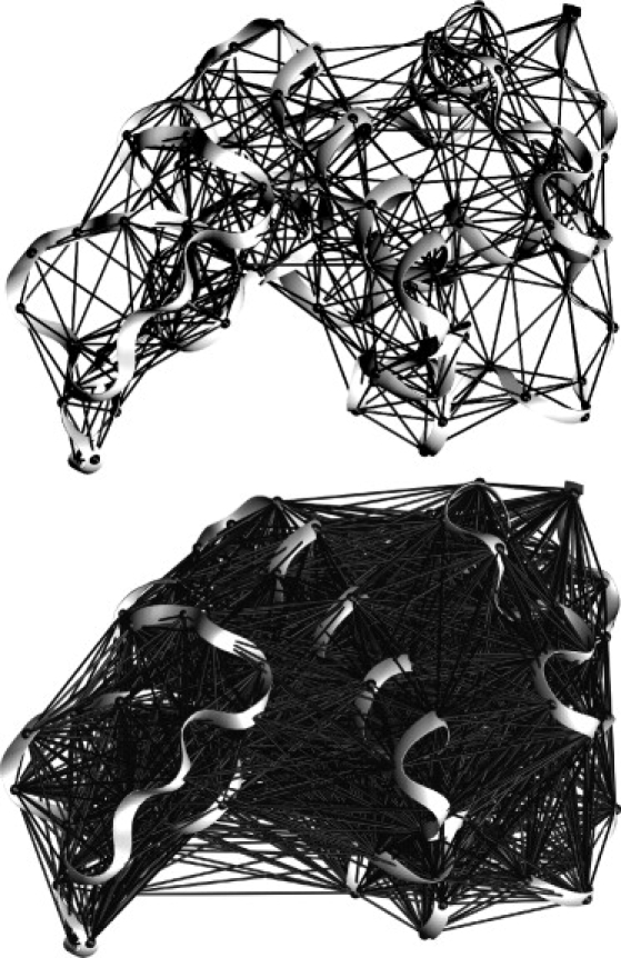
Isolated Lysozyme (PDB ID: 3LZT) rendered with ANM interactions between atoms with 8 Å and 16 Å cutoffs on the top and bottom, respectively.

In addition to the C_α-based elastic network models, all protein systems are also studied with the Gaussian network model (GNM) introduced by Haliloglu et al. (37); this is a different model that replaces the 3N dimensional Hessian, where N is the number of atoms, with an N dimensional Kirchoff matrix,

$$\Gamma =\{\begin{array}{ll}-1\hfill & \mathrm{if}\mathrm{i}\ne \mathrm{j}\text{and}{R}_{\mathrm{ij}}\le R_{\text{cut}}\hfill \\ 0\hfill & \mathrm{if}{R}_{\mathrm{ij}}>R_{\text{cut}}\hfill \\ -\sum _{\mathrm{i},\mathrm{j}\ne \mathrm{i}}{\Gamma }_{\mathrm{ij}}\hfill & \mathrm{if}\mathrm{i}=\mathrm{j}\hfill \end{array}.$$

The N × N variance-covariance matrix is determined similarly from the frequencies and the eigenvectors that correspond to isotropic vibrations of the atoms, and the theoretical temperature factors (isotropic) are simply proportional to the diagonal entries of this matrix.

Implementation and boundary conditions

In addition to the isolated molecule case (referred to as ISL below), all of the elastic network models discussed above (HCA, ANM, and GNM) have been implemented for crystalline state calculations under several boundary conditions. The first, referred to as ASYMPBC, is based on the asymmetric unit (e.g., see the red region in Fig. 2), where all interactions within itself and with neighboring molecules in the crystal are included in the Hessian matrix. The Hessian has the same dimension as for the isolated molecule; i.e., if atoms i and j in different asymmetric units are within the cutoff, K_ij has an entry for that interaction. The second is similar to the first, but instead of using the asymmetric unit, the entire unit cell is used, which may include several asymmetric units (e.g., large, solid black and gray spheres in Fig. 2); this is referred to as P1PBC. The third utilizes the Born-von Kármán (BVK) boundary condition to naturally incorporate lattice vibrations, and will be elaborated below.

Figure 2.

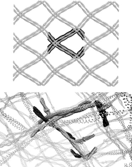
Crystal structure of tropomyosin (PDB ID: 2TMA) in the C_α representation. The top figure is rendered orthographically with the a axis pointing out of the page; the primitive cell is in large solid spheres and the 26 nearest neighbors are shown with smaller open spheres. The bottom figure is in perspective with a slightly rotated orientation, zoomed in on the central unit cell; the primitive unit cell has four asymmetric units (space group P2₁2₁2): one is shown with solid black spheres (color online) and the other three are shown with solid gray spheres. Tropomyosin is involved in actin regulation and consists of two long, coiled α-helices that resemble a floppy noodle when taken alone. In contrast, the crystal structure has many intermolecular interactions, which yields a structure resembling chicken wire. This crystal structure is low-resolution and not included in the set of 83 proteins.

The crysFML library (51) is used for all necessary symmetry operations for crystal construction. Depending on whether the entire vibrational spectrum is desired, ARPACK (52) or LAPACK are used to determine the eigenvectors and eigenvalues. Since the variance-covariance matrix is expected to be dominated by low-frequency modes, in addition to all-modes calculations whenever possible, calculations are also carried out in which only the first 5% (i.e., lowest frequencies) of the modes is used.

Born-von Kármán boundary conditions

From a computational point of view, biological crystals used for diffraction studies are vast. With n atoms in the unit cell and N unit cells, where N is ∼10¹², simulating motions of a crystal requires a proper treatment of the periodicity. The classical theory of lattice vibrations was formulated by Born and von Kármán in the early 20th century (53,54) and has been discussed in detail in several classical texts (41,55,56). This approach was recently applied to ribonuclease A (57) using the CHARMM potential and lysozyme (40) using the HCA model. For the C_α elastic network models a dynamic matrix (D) is constructed with the same potentials as discussed in Elastic Network Models (ENM) with an added phase factor that depends on the dot product of the wave vector q and the displacement vector connecting the two interacting atoms,

$$\mathbf{D}(\mathrm{k}{\mathrm{k}}^{\prime },\mathbf{q})=\sum _{{\mathrm{l}}^{\prime }}{\mathbf{K}}_{0{\mathrm{l}}^{\prime }}^{\mathrm{k}{\mathrm{k}}^{\prime }}{e}^{\mathrm{i}\mathbf{q}\cdot (\mathbf{R}\left({\mathrm{k}}^{\prime }{\mathrm{l}}^{\prime }\right)-\mathbf{R}\left(\mathrm{k}0\right))}.$$ (10)

Here ${\mathbf{K}}_{0{\mathrm{l}}^{\prime }}^{\mathrm{k}{\mathrm{k}}^{\prime }}$ represents the force constant for the interaction between atoms k and k′, which are in the central and l′ unit cells, respectively. In our implementation, this essentially amounts to the same construction as P1PBC introduced above, but with the added phase factor; the dynamic matrix and the P1PBC matrix are exactly the same for q = 0. In contrast to solution phase computations, the minimum image convention (58), which avoids interactions of an atom with its own image, is not enforced. Since the dynamic matrix D is Hermitian, the eigenvectors are complex and the eigenvalues (ω²) are real,

$${\mathbf{L}\left(\mathbf{q}\right)}^{†}\mathbf{D}\left(\mathbf{q}\right)\mathbf{L}\left(\mathbf{q}\right)=\Lambda \left(\mathbf{q}\right),$$ (11)

where the eigenvectors of relative displacement and frequencies now depend on the wavevector, q. Three zero eigenvalues for q = 0 become finite with finite wavevectors and depend most strongly on the value of q among all modes; termed acoustic modes, the variation of the corresponding frequencies with q as q approaches zero can be used to compute the speed of sound in the crystal (see the Supporting Material). The other modes, optical modes, typically show less significant q-dependence in the frequency. The variance-covariance matrix,

$$\langle {\mathbf{uu}}^T\rangle =k_{\mathrm{B}}T\times {\langle \mathbf{L}{\Lambda }^{-1}{\mathbf{L}}^{†}\rangle }_{\mathrm{q}},$$ (12)

is computed as an average over the wave vectors sampled in the first Brillouin zone (BZ), and only the real components of the variance-covariance matrix are used for comparisons to experiments. With regard to the reciprocal lattice vectors (a^∗,b^∗,c^∗) that are associated with the crystal lattice, the first BZ spans the parallelepiped defined by −0.5 to 0.5 for each direction. Since we are interested in applying this approach to a set of 83 proteins (discussed below), we approximate the BZ with a grid of 27 wave vectors distributed in the positive octant constructed from permutations of 0.00, 0.25, and 0.50 in each reciprocal lattice vector direction. This sampling is found to be adequate when compared to more complete sampling with finer grids (see the Supporting Material for additional discussions).

Set of structures and comparisons to experiment

In this study, we use the same set of 83 diverse, ultra-high resolution structures used by Kondrashov et al. (39), who compared various NMA approaches for isolated molecules. The number of C_α atoms in the unit cell ranges from 68 (Protein Data Bank (PDB) ID: 1VBW) to 5200 (PDB ID: 1O7J), thus the test set includes both small and very large systems. In the study of Kondrashov et al. (39), isotropic and anisotropic comparisons were carried out for all residues not involved in crystal contacts and had an occupancy of 1.0; 12,348 residues met these criteria (39). Since the crystal environment is explicitly taken into considerations in our calculations, we can make the same types of comparisons for the entire set of residues with an occupancy of 1.0; this increases the comparable set to 16,853 residues. The theoretical values for each residue are determined from the 3 × 3 diagonal blocks of the variance-covariance matrices computed with the ENMs discussed above,

$$\langle {\mathbf{u}}_{\mathrm{i}}{\mathbf{u}}_{\mathrm{i}}^T\rangle ={\mathbf{C}}_{\mathrm{i}\mathrm{i}}=\left(\begin{array}{ccc}\langle \mathit{\delta }{x}_{\mathrm{i}}^2\rangle & \langle \mathit{\delta }{x}_{\mathrm{i}}\mathit{\delta }{y}_{\mathrm{i}}\rangle & \langle \mathit{\delta }{x}_{\mathrm{i}}\mathit{\delta }{z}_{\mathrm{i}}\rangle \\ & \langle \mathit{\delta }{y}_{\mathrm{i}}^2\rangle & \langle \mathit{\delta }{y}_{\mathrm{i}}\mathit{\delta }{z}_{\mathrm{i}}\rangle \\ & & \langle \mathit{\delta }{z}_{\mathrm{i}}^2\rangle \end{array}\right).$$ (13)

These blocks are symmetric about the diagonal and thereby generate six unique entries for the anisotropic displacement parameters (ADP) for each residue (i). The isotropic temperature factor (B-factor) is the average of the three diagonal entries of Eq. 13. For all comparisons described below, the averages are computed over the set of proteins weighted by the number of residues available for comparison in each protein. The results are reported for both the full set of 83 and a subset of the 33 smallest proteins with the number of residues in the primitive unit cell ≤500; this facilitates both the more expensive BVK calculations with the full spectrum of modes and an assessment of the effect of system size.

We note that there are some concerns about using temperature factors to calibrate models for protein dynamics because it is well known that the temperature factors include many contributions other than thermal fluctuations, such as static disorders in the crystal (41,59). Indeed, there is argument that thermal fluctuations in the crystalline state are not the dominant contribution to the isotropic B-factors (40,60). However, as also recognized by others (40), the static disorders are also largely correlated with the intrinsic flexibility of the protein, which is perhaps why normal mode models that focus on low-frequency modes have been reasonably successful in reproducing the experimental isotropic and anisotropic temperature factors (36,38,39). Therefore, we believe that temperature factors from very high resolution x-ray diffraction, although not perfect, remain as the most well-defined experimental data for characterizing theoretical models for protein dynamics in the crystalline state.

Comparison to isotropic temperature factors

Similar to the study of Kundu et al. (36), a linear correlation coefficient is used for comparisons between the theoretical model and experiment for each protein,

$$\mathit{\rho }=\frac{{\sum }_{\mathrm{j}=1}^M(B_{\mathrm{j}}^{\text{exp}}-\langle B^{\text{exp}}\rangle )(B_{\mathrm{j}}^{\text{thr}}-\langle B^{\text{thr}}\rangle )}{\sqrt{{{\sum }_{\mathrm{j}=1}^M(B_{\mathrm{j}}^{\text{exp}}-\langle B^{\text{exp}}\rangle )}^2{\sum }_{\mathrm{i}=1}^M{(B_{\mathrm{i}}^{\text{thr}}-\langle B^{\text{thr}}\rangle )}^2}},$$ (14)

where M is the number of usable C_α atoms and B are the experimental (exp) and theoretical (thr) isotropic temperature factors; individual values are labeled by the index and the average value for the protein is in brackets.

Comparison to anisotropic temperature factors

For the comparisons of the ADPs between the experiment and theory, the ellipsoidal probability distributions are compared for direction and overall similarity. The ellipsoid is related to the eigenvalues and eigenvectors of the 3 × 3 matrices constructed from the ADPs. The theoretical anisotropic temperature factors are compared to experiment for residues that have an experimental anisotropy ≤0.5, where the anisotropy is defined as the ratio of the smallest to largest eigenvalues of the atomic covariance matrix (Eq. 13); 6619 experimental observations satisfy this criteria. For these comparisons, both experimental and theoretical ADPs are normalized by their trace. The directionality of the ellipses is evaluated by the dot product of the major axes. A modified form of an overlap score that measures the similarity of two probability distributions (61) is used. The correlation coefficient (cc) that is related to the overlap integral of two probability distributions is defined as (61)

$$\text{cc}(\mathbf{U},\mathbf{V})=\frac{{\left(\text{det}{\mathbf{U}}^{-1}\text{det}{\mathbf{V}}^{-1}\right)}^{\frac{1}{4}}}{\sqrt{\frac{1}{8}(\text{det}{\mathbf{U}}^{-1}+\text{det}{\mathbf{V}}^{-1})}},$$ (15)

where U and V are the experimental and theoretical ADP tensors, respectively. The modified coefficient (39),

$${\text{cc}}_{\text{mod}}(\mathbf{U},\mathbf{V})=\frac{\text{cc}(\mathbf{U},\mathbf{V})-\text{cc}(\mathbf{U},{\mathbf{V}}^{\ast })}{1-\text{cc}(\mathbf{U},{\mathbf{V}}^{\ast })},$$ (16)

is 1.0 for perfect overlap, and 0.0 if the two ellipses are perfectly misaligned; V^∗ is generated by taking the eigenvectors of U and using the eigenvalues, with the largest and smallest switched, of V to define the two ellipses with perfect misalignment.

Additional comparisons of different ENMs

In addition to the comparisons to experimental crystallographic data, several other types of quantities are used to further explore the performance of various ENMs and the effect of the crystal environment on the vibrational motions of proteins.

Long-range correlations in proteins

To complement the comparison of ADPs, which reflect correlated motions in proteins via the anisotropy of local atomic motions, we explicitly compare the normalized atomic correlations over the entire protein,

$${\Phi }_{\mathrm{i}\mathrm{j}}=\frac{\langle \mathit{\delta }{r}_{\mathrm{i}}\mathit{\delta }{r}_{\mathrm{j}}\rangle }{\sqrt{\langle \mathit{\delta }{r}_{\mathrm{i}}^2\rangle \langle \mathit{\delta }{r}_{\mathrm{j}}^2\rangle }},$$ (17)

where each element of the atomic correlation matrix (Φ) is determined from an average of the diagonal elements of the 3 × 3 blocks of the variance-covariance matrix that describe the correlated motions of different atoms, i and j, and normalize by the magnitude of the fluctuations of each atom. Using Φ rather than the variance-covariance matrix makes the comparison straightforward because it has no dependence on the orientation or the scaling of the force constant in different ENMs.

Scaling of cumulative density of states and the heat capacity

As discussed in several previous studies (37,57,62), comparing the scaling behavior of vibrational density of states and heat capacity to theoretical results of simple models of crystals provide insights into the unique dynamical nature of proteins relative to simple molecules. Therefore, we expect that the scaling behavior can also be used to contrast different coarse-grained protein models.

The density of states, g(ν), is defined such that g(ν)dν gives the number of frequencies between ν and ν + dν. In this investigation, a normalized (fractional) g(ν) is constructed via a 75-bin histogram that spans the entire spectrum for the various ENMs described above; the bin width (Δν) is 1/74 of the maximum frequency. The normalized cumulative density of states, G(ν),

$$G\left({\nu }_f\right)=\sum _{\mathrm{i}}^{f}g\left({\nu }_{\mathrm{i}}\right),$$ (18)

varies from the fraction of zero frequency modes (∼0.0) to 1.0 with each point separated by the bin width. The (normalized) molar heat capacity (C_V) is computed from the fractional density of states,

$$C_V\left(T\right)=\frac{h^2}{{\text{RT}}^2}\sum _{\mathrm{i}}\frac{1}{2(\text{cosh}\left(\frac{h{\nu }_{\mathrm{i}}}{\text{RT}}\right)-1)}g\left({\mathit{\nu }}_{\mathrm{i}}\right)\Delta \mathit{\nu },$$ (19)

and varies from zero to the gas constant, R (1.99 cal/mol·K). The power law is determined for G(ν) at low frequencies (G(ν) ∼ ν^b where b is the exponent of interest) and the heat capacity at low temperature (C_V ∼ T^b′) is determined from the log-log fit for the region of the curve that falls between 0.03 and 0.20 for G(ν) and between 0.01 and 0.10R for C_V. This choice is most convenient when considering the variable nature of the force constant in the ENMs as discussed in Elastic Network Models (ENM).

Results and Discussion

Isotropic correlations

GNM

In the study of Kundu et al. (36), the Gaussian network model (GNM) (37) was applied to a set of 113 proteins. In that study, using all frequencies and a 7.3 Å cutoff, the average correlation was found to increase from 0.59 to 0.66 when the crystal environment was treated approximately by extending the isolated molecule with nearest neighbors. In a similar study, Kondrashov et al. (63) developed an improved GNM model, referred to as “CNM”, that added chemical information without increasing the computational cost of the problem. By including the crystal environment with periodic boundary conditions about the asymmetric unit, as described in Implementation and Boundary Conditions, they found a similar average correlation for the GNM model of 0.66 with a 7.5 Å cutoff for a different set of 98 high resolution crystallographic data using the lowest 100 modes.

In this study, with the 83 proteins and various boundary conditions discussed in Implementation and Boundary Conditions, we find qualitatively the same behavior for the GNM calculations. As shown in Table 1, when all the normal modes are used, the average correlation increases from 0.58 for the isolated molecule to 0.63 with ASYMPBC. P1PBC does not further improve the agreement and also gives an average correlation of 0.63. Using 5% of the normal modes slightly reduces the correlation, but the trends remain the same; e.g., the correlation increases from 0.54 for ISL to 0.61 for ASYMPBC. The average correlation is reduced for the subset of 33 smallest proteins (≤500 residues in the primitive unit cell) relative to the full set, and the reduction is most significant for P1PBC when 5% of the modes is used, decreasing from 0.60 for the entire list of 83 proteins to 0.50 for the 33-subset. This is probably because for smaller proteins the dominance of low-frequency modes is not as transparent as in larger proteins, especially when crystal contacts are present. The relatively rigid nature of smaller proteins is also consistent with the observation that the effect of the crystal environment is less significant on the correlation; the correlation increases by ∼0.02 going from ISL to P1PBC for the 33-subset, whereas the increase is ∼0.05 for the full set. The isotropic correlation computed with the BVK boundary condition is very similar to that of P1PBC, regardless of the size of the system and the number of modes included.

Table 1.

Correlation coefficients between experimental isotropic temperature factors and calculated values using various C_α-based ENMs and different ways of treating the crystal environment

Model	ISL∗	ASYMPBC∗	P1PBC∗	BVK∗
GNM†	0.54 (0.58)	0.61 (0.63)	0.60 (0.63)	0.59 (−)
ANM10‡	0.46 (0.51)	0.54 (0.59)	0.54 (0.60)	0.55 (−)
ANM16§	0.47 (0.57)	0.50 (0.60)	0.50 (0.59)	− (−)
HCA	0.53 (0.56)	0.66 (0.67)	0.66 (0.68)	0.66 (−)
33-Subset
GNM†	0.48 (0.56)	0.52 (0.59)	0.50 (0.58)	0.50 (0.58)
ANM10‡	0.41 (0.46)	0.46 (0.52)	0.46 (0.52)	0.46 (0.53)
ANM16§	0.45 (0.55)	0.39 (0.49)	0.40 (0.48)	0.40 (0.47)
HCA	0.49 (0.53)	0.60 (0.63)	0.60 (0.63)	0.60 (0.63)

As discussed in Set of Structures and Comparisons to Experiment, each value is a weighted average for the set (Eq. 14). The values for the entire set of 83 proteins are shown first, followed by results for the subset of the 33 smallest proteins (≤500 residues in the primitive unit cell). The values without parentheses are calculated with 5% of the modes and those with parentheses are calculated with all modes.

^∗ISL is for isolated systems without the crystal environment; ASYMPBC, P1PBC, and BVK are different ways of treating the crystal environment (see Implementation and Boundary Conditions).

^†7.3 Å cutoff.

^‡10.0 Å cutoff.

^§16.0 Å cutoff.

ANM and HCA

For a given model, the average correlation is insensitive to different boundary conditions used to treat the crystal environment. For HCA, for example, when 5% of the modes is used, the average correlations for the entire test set are all ∼0.66 with ASYMPBC, P1PBC, and BVK. These are significantly higher than the value of 0.53 with ISL, which reinforces the finding based on GNM that including the crystal environment is important for comparison to crystallographic data.

Interestingly, including the crystal environment also helps to better contrast different ENMs. Using all of the modes, ANM₁₆ has a slighter higher average correlation (0.57) than both ANM₁₀ (0.51) and the HCA model (0.56) for the ISL case. Including the crystal environment improves the correlation for all models, although the effect is more apparent for HCA: HCA increases to 0.67 (0.68) with ASYMPBC (P1PBC) and both ANM models increase to ∼0.60. Using a longer cutoff for ANM (15–24 Å) has been previously prescribed (48) for better performance, but this was based on comparisons of the ISL results to the crystallographic B factors, which is not a consistent benchmark. As shown in Fig. 3, the ANM results improve as the cutoff increases from 8 to 16 Å for the ISL case, but this improvement is in stark contrast to the behavior when the crystal environment is included in the calculations, which give a nearly constant value of 0.6 for all cutoffs. Another signature for the unphysical nature of ANM₁₆ is found when the small proteins (33 subset) are studied. As shown in Table 1, whereas the average correlation improves for both HCA and ANM₁₀ as the crystal environment is taken into consideration (e.g., from 0.53 for ISL to 0.63 for P1PBC with the HCA model), the correlation decreases for ANM₁₆ (e.g., from 0.55 for ISL to 0.48 for P1PBC).

Figure 3.

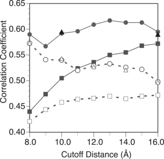
Correlation coefficient between the ANM and experimental isotropic temperature factors as a function of the ANM cutoff distance using various ways of treating the crystal environment. Each point (squares, circles, and triangles) represents a weighted average for the set of 83 proteins (Eq. 14). The solid lines and shapes include all normal modes in the calculations whereas the dashed lines and open shapes include only 5% of the modes for each protein. The squares, circles, and triangles are for the ISL, ASYMPBC, and P1PBC boundary conditions, respectively. Comparing the boundary conditions, including the crystal environment via periodic boundary conditions, clearly improves the agreement with experiment, and the largest gains are at shorter cutoff distance. Both ASYMPBC and P1PBC yield similar agreement for both set of calculations (5% and 100%). As discussed in the text, using 5% of the modes dramatically reduces the agreement, and this behavior has a strong dependence on the cutoff distance.

Using only the low frequency modes (5%) reduces the average correlations slightly (∼0.01–0.04) for the HCA, but significantly for ANM (∼0.05–0.10) for all boundary conditions. This is most significant for ANM₁₆; as shown in Fig. 4, the agreement between the 5%-modes and the all-modes results gets worse as the cutoff in ANM increases. Apparently, as the cutoff increases and the system becomes increasingly restrained (see Fig. 1 as an illustration), the lowest 5% of the modes no longer dominates the variance-covariance matrix, which is an unphysical feature of the model.

Figure 4.

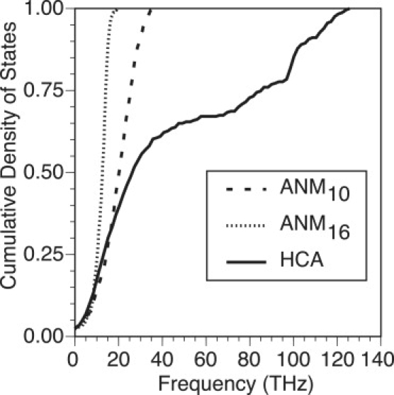
Calculated cumulative density of states for an isolated (ISL) PDZ2 domain of syntenin (PDB ID: 1R6J) using ANM₁₀, ANM₁₆, and HCA. For each calculation, the force constant is scaled to best fit the experimental isotropic temperature factors, which defines the range of frequencies for each model. In contrast to ANM₁₀ and ANM₁₆ the cumulative density of states for HCA has distinct features due to the distance-dependence of the force constant.

Anisotropic correlations

Average anisotropy

The average anisotropy, defined as the ratio of the smallest to largest eigenvalue of the 3 × 3 ADP tensor, is the crudest comparison between theoretical and experiment anisotropic temperature factors, but some general trends can be captured. For a given ENM, the degree of anisotropy decreases as the crystal environment and more modes are taken into account (see Table 2). For example, for HCA, the average anisotropy is 0.41 with ISL and 0.50 with P1PBC when all modes are considered; with only 5% of the modes, the corresponding values are 0.26 and 0.42, respectively, indicating a higher degree of anisotropy. With the smaller proteins (33 subset), the average anisotropy is higher (i.e., lower numerical values), although the general trends regarding the effects of different boundary conditions and number of modes remain the same. Based on the observed trends, the best agreement with the experimental data (0.54) is found with HCA/ANM₁₀ and the BVK boundary condition. Whereas ANM₁₆ gives similar results to other models when 5% of the modes is used, the average anisotropy is significantly reduced (i.e., higher numerical values) when all modes are used (e.g., 0.66 with P1PBC); this is largely expected considering the large number of interactions each atom is engaged in with this model.

Table 2.

Comparison of experimental anisotropic displacement factors (ADPs) and calculated values using various C_α-based ENMs and different ways of treating the crystal environment

Model	ISL∗	ASYMPBC∗	P1PBC∗	BVK∗
Anisotropy: 0.54
ANM10†	0.24 (0.43)	0.31 (0.50)	0.39 (0.52)	0.50 (−)
ANM16‡	0.21 (0.57)	0.29 (0.63)	0.40 (0.66)	− (−)
HCA	0.26 (0.41)	0.33 (0.47)	0.42 (0.50)	0.52 (−)
33-Subset anisotropy: 0.54
ANM10†	0.16 (0.39)	0.23 (0.46)	0.31 (0.48)	0.46 (0.52)
ANM16‡	0.12 (0.50)	0.19 (0.60)	0.30 (0.63)	0.47 (0.64)
HCA	0.18 (0.37)	0.25 (0.44)	0.35 (0.47)	0.49 (0.52)
Dot product
ANM10†	0.64 (0.64)	0.69 (0.66)	0.71 (0.68)	0.73 (−)
ANM16‡	0.63 (0.63)	0.66 (0.64)	0.69 (0.67)	− (−)
HCA	0.65 (0.67)	0.70 (0.69)	0.72 (0.71)	0.74 (−)
33-Subset dot product
ANM10†	0.64 (0.64)	0.67 (0.67)	0.69 (0.68)	0.71 (0.69)
ANM16‡	0.64 (0.65)	0.66 (0.68)	0.69 (0.70)	0.70 (0.70)
HCA	0.65 (0.67)	0.69 (0.69)	0.71 (0.70)	0.73 (0.71)
ccmod
ANM10†	0.50 (0.57)	0.62 (0.61)	0.67 (0.64)	0.70 (−)
ANM16‡	0.45 (0.56)	0.55 (0.55)	0.62 (0.57)	− (−)
HCA	0.54 (0.63)	0.65 (0.67)	0.70 (0.69)	0.72 (−)
33-Subset ccmod
ANM10†	0.43 (0.57)	0.53 (0.62)	0.60 (0.63)	0.67 (0.64)
ANM16‡	0.33 (0.60)	0.44 (0.59)	0.54 (0.60)	0.61 (0.59)
HCA	0.47 (0.61)	0.58 (0.66)	0.65 (0.67)	0.70 (0.67)

As discussed in the text, each value is a weighted average; dot product is between the major axes of the calculated and experimental ADPs, and the definition of the overlap score (cc_mod) is given in Eq. 16. For each of the three comparisons, results for the full set of 83 proteins are above those for the subset of 33 smallest systems. The values without parentheses are calculated with 5% of the modes and those with parentheses are calculated with all modes.

^∗ISL is for isolated systems without the crystal environment; ASYMPBC, P1PBC, and BVK are different ways of treating the crystal environment (see Implementation and Boundary Conditions).

^†10.0 Å cutoff.

^‡16.0 Å cutoff.

ADP ellipsoidal comparisons

As described in Set of Structures and Comparisons to Experiment, the ellipses are compared using directionality (dot product of major axes) and a scalar that measures the overlap of the two probability densities (cc_mod). As shown in Table 2, for both ANM and HCA, the agreement with experiment as reflected by the dot product improves slightly with the inclusion of the crystal environment. Using 5% or all of the modes does not have as much of an effect on the average dot product for either the full set of 83 or the subset of 33 proteins. Most models give a value at ∼0.70.

For the overlap coefficient (cc_mod), the effect of the crystal environment is more visible and most significant when 5% of the modes is used: the agreement with experiment generally increases by ∼0.2 going from ISL to the BVK boundary condition regardless of the ENM; both HCA and ANM₁₀ outperform ANM₁₆ by a notable degree. Using 100% of the modes renders ANM₁₆ insensitive to the crystal environment with a constant value ∼0.56 (0.60) for the set of 83 (33) proteins. By contrast, the agreement improves for HCA and ANM₁₀ when the crystal environment is included, and HCA with the BVK boundary condition yields the best agreement with experiment, leading to a value ∼0.70.

Long-range correlations

As an illustration, we examine the atomic (C_α) correlations for the PDZ2 domain of syntenin, which was also examined in Kondrashov et al. (39). Using ANM₁₆ and block normal mode calculation (64) with the CHARMM force field (65), Kondrashov et al. found fairly similar features between the two approaches although the magnitude of off-diagonal correlations for ANM₁₆ was significantly lower than that for the all-atom result. For the ISL case, plotted in Fig. 5 a, there is a similar contrasting behavior between ANM₁₆ (upper triangle) and HCA (lower triangle), whereby the range of correlated motions is very much washed out for ANM₁₆ due to the large number of strong interactions. Both HCA and ANM₁₀ (data not shown) yield magnitudes of correlation that are in good agreement with the CHARMM result (39).

Figure 5.

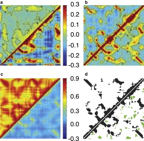
Calculated atomic correlations (Eq. 17) and contact maps for the PDZ2 domain of syntenin (PDB ID: 1R6J) using various C_α-based ENMs and different ways of treating the crystal environment. The residue number is plotted along the x and y axes and ranges from 1 to 82 in all plots. Atomic correlations are shown in a–c (note the difference in scale between c and a/b): (a) ISL results obtained with ANM₁₆ (HCA) are shown in the upper (lower) triangle. (b) ASYMPBC and P1PBC results obtained using HCA are plotted above and below the diagonal, respectively. (c) Correlations computed with BVK and 27 wavevectors using only the three acoustic modes are shown above the diagonal and results obtained with all modes below the diagonal. (d) The Kirchoff matrix for the ISL and ASYMPBC cases (using a cutoff of 10.0 Å) are plotted above and below the diagonal, respectively; blue indicates off-diagonal contacts that exist in the ISL case and green highlights contacts introduced via the crystal environment.

Regarding atomic correlations in the crystalline state, the overall trend observed for this system is that including the crystal environment tends to decrease the magnitude of negative correlations and there are significant differences between different treatments. Fig. 5, b and c, illustrates the situation using the HCA results. As shown in Fig. 5 b, P1PBC yields similar regions of significant correlation as ASYMPBC, but the correlations are all shifted to be more positive. This particular crystal structure (66) has two asymmetric units per unit cell, thus the P1PBC treatment includes additional correlations due to the relative motions of the two asymmetric units. This trend is further enhanced when BVK is used (see Fig. 5 c), where now the correlated motion associated with the acoustic modes (upper triangle) yields entirely positive correlations due to the nature of the lattice modes coupling the motion across different unit cells; due to this strong contribution of positive correlation there is no longer any negative correlation for the BVK boundary condition (lower triangle). As expected, the correlations associated with the optical modes are very similar to that found with P1PBC (see the Supporting Material). Moreover, as shown in the Supporting Material, the correlation matrix associated with the acoustic modes depends more strongly on the number of wavevectors sampled in the first BZ but converges quickly as the number of wavevectors is increased. This dependence is not as apparent when both acoustic and optical contributions are considered together.

Scaling of cumulative density of states and the heat capacity

As shown in Table 3, the scaling behavior of the cumulative density of states and molar heat capacity is similar between the full set of 83 and subset of 33 proteins for ISL, ASYMPBC, and P1PBC. Therefore, the BVK case is only analyzed for the 33-subset, and discussions are also focused on this smaller set.

Table 3.

Scaling exponent of the cumulative density of states and heat capacity determined using various C_α-based ENMs and different ways of treating the crystal environment

Model	ISL∗	ASYMPBC∗	P1PBC∗	BVK∗
Gν
GNM†	2.01 (0.19)	2.38 (0.30)	2.24 (0.24)
ANM10‡	2.14 (0.33)	2.79 (0.32)	2.65 (0.27)
ANM16§	4.00 (0.89)	7.56 (1.96)	7.35 (1.56)
HCA	1.87 (0.24)	2.44 (0.24)	2.41 (0.21)
33-Subset: Gν
GNM†	1.98 (0.24)	2.50 (0.39)	2.31 (0.34)	2.17 (0.28)
ANM10‡	2.09 (0.40)	2.89 (0.40)	2.68 (0.36)	2.52 (0.32)
ANM16§	3.96 (1.08)	8.60 (2.28)	8.18 (1.77)	7.53 (1.45)
HCA	1.78 (0.28)	2.53 (0.33)	2.45 (0.29)	2.38 (0.26)
CV
GNM†	2.52 (0.22)	2.94 (0.29)	2.68 (0.22)
ANM10‡	2.29 (0.38)	2.88 (0.27)	2.72 (0.24)
ANM16§	3.54 (0.49)	4.43 (0.23)	4.33 (0.23)
HCA	2.15 (0.22)	2.62 (0.16)	2.52 (0.14)
33-Subset: CV
GNM†	2.56 (0.29)	3.11 (0.33)	2.77 (0.29)	2.50 (0.20)
ANM10‡	2.24 (0.46)	2.98 (0.34)	2.79 (0.32)	2.60 (0.27)
ANM16§	3.47 (0.54)	4.55 (0.21)	4.46 (0.22)	4.30 (0.19)
HCA	2.12 (0.26)	2.71 (0.19)	2.58 (0.17)	2.46 (0.14)

Numbers in parentheses are the root mean-square deviations. For each of the three comparisons, results for the full set of 83 proteins are above those for the subset of 33 smallest systems. All frequencies are included in the G_ν and C_V calculations although only data in certain frequency ranges are included for determining the exponents (see Additional Comparisons of Different ENMs).

^∗ISL is for isolated systems without the crystal environment; ASYMPBC, P1PBC, and BVK are different ways of treating the crystal environment (see Implementation and Boundary Conditions).

^†7.3 Å cutoff.

^‡10.0 Å cutoff.

^§16.0 Å cutoff.

Cumulative density of states

For the ISL case, G_ν scales (G_ν ∼ ν^b) as 1.98, 1.78, and 2.09 for GNM, HCA, and ANM₁₀, respectively. These values are in good agreement with the value of 2.0 calculated for a smaller set with normal mode analysis by ben Avraham (62). The value for GNM here is slightly higher than the value of 1.63 found by Haliloglu et al. (37); the intermediate portion of the curve was used in that calculation, which is expected to reduce the scaling exponent slightly. The scaling exponent is significantly higher for ANM₁₆ with a value of 3.96. The values increase for all models as the crystal environment is included. ASYMPBC yields the highest values that are ∼2.5 for both GNM and HCA, which are below the value of 2.89 for ANM₁₀ and 8.60 for ANM₁₆. These values are slightly reduced with P1PBC and BVK. ANM₁₆ is significantly higher for all boundary conditions.

We note that the distance-dependence of the force constant in HCA leads to distinct features in the density of states compared to ANM. As shown earlier in Fig. 4 using the PDZ2 domain of syntenin as an example, whereas G_ν increases sharply as a function of frequency for both ANM₁₀ and ANM₁₆, the HCA result increases only slowly to 1.0 via a series of steps after the initial quick rise at low frequencies. This difference is found consistently for other proteins and boundary conditions, which is in line with the previous observation that ENMs with a uniform force constant give qualitatively different frequency distributions compared to models that distinguish covalent and nonbonded interactions (67).

Heat capacity

Meinhold et al. (57) found that C_V ∼ T^1.68 for ribonuclease A under the BVK boundary condition with an all-atom normal mode calculation where the sampling of the BZ was confined to the axes of the reciprocal lattice vectors; their result was found to compare well with experiments that yield a range of b = 1.60–1.77 (57) for hydrated globular proteins. Focusing on the BVK boundary condition, GNM, ANM₁₀, and HCA in our study lead to similar values (2.50, 2.60, and 2.46) for the 33 proteins and are all significantly higher than the all atom results and experimental values (57), pointing to one limitation of these simple protein models. ANM₁₆ gives the most dramatic difference with a power law of C_V ∼ T^4.30, which is even steeper than the Debye behavior of cubic scaling for simple lattices (68).

Conclusions

In this investigation, several simple C_α-based elastic network models are applied under several boundary conditions that either ignores or includes the crystal environment in different ways. To assess the performance, the computed temperature factors are compared to experiment for 83 ultra-high resolution crystallographic data sets. For all models, treating proteins in the crystalline state is found to yield better agreement with experiments. The three treatments of the crystal environment (ASYMPBC, P1PBC, BVK) lead to similar results for the isotropic temperature factors but notable differences for the anisotropic displacement factors; the average anisotropy (over all atoms with 1.0 occupancy) has the strongest dependence on the crystal treatment where BVK yields the best agreement with experiment. Atomic correlations over the entire protein are clearly affected by the presence of the crystal contacts and also fairly sensitive to the way that the crystal environment is treated. Significant differences are also found between the different treatments of the crystal environment when the scaling behaviors of cumulative vibrational density of states and heat capacity are considered.

This study quantitatively highlights the point that when validating approximate models for proteins using experimental data such as the x-ray diffraction temperature factors, it is crucial to treat the protein system in an environment consistent with experiment, which has also been discussed in previous (36,69) and recent studies (40,60). For example, for protein in isolation, ANM seems to yield the best agreement with the experimental isotropic temperature factors when the cutoff is increased to 16.0 Å, but this is misleading. Without the crystal environment, the molecule is expected to behave differently, and adding more and more strong interactions inappropriately restrains the isolated molecule. Although this may lead to apparently more accurate isotropic temperature factors as compared to the experimentally determined values for the crystalline state, it is clearly shown here that the model has several unphysical features: with ANM₁₆, using 5% of the normal modes leads to isotropic factors significantly different from those calculated using all modes, and including the crystal environment in fact makes the ANM₁₆ results in worse agreement with experimental data. Therefore, a 10 Å cutoff is recommended for general application of ANM with the C_α representation. The HCA model, which is physically more appealing with the strength of interaction decreasing as a function of atomic separation, outperforms all other models, including GNM, when the crystal environment is treated for the computation of both isotropic and anisotropic temperature factors. The transferability of models optimized for crystals to isolated proteins in solution is an interesting topic for future investigations. It is possible that the differences in solvent accessibility could yield differences in the model parameters, and the extent of this can be determined through comparisons to NMR experiments and all-atom molecular dynamics simulations.

The observation that calculated atomic correlations are significantly affected even in a relatively small protein by the presence of the crystal environments suggests that explicitly treating the system in the crystalline state is crucial when considering protein dynamics in structural refinement type of applications; we note that the dynamical nature of protein in the crystalline state is reflected in both thermal fluctuations and static disorders, thus a meaningful theoretical model should attempt to describe both (36,40,41,60,69). In this regard, the BVK boundary condition, although more expensive than ASYMPBC and P1PBC, is required to simulate experimental observables such as the dispersion relations, speed of sound, and the effects of correlated motions on x-ray scattering. From calculations of the dispersion relations and speed of sound, which are described in the Supporting Material, ANM and HCA are shown to capture key trends with respect to all-atom calculations (57), although the results and the scaling exponents of heat capacity also highlight gaps between all-atom models and the simplified models explored here. It would be interesting to explore the performance of other coarse-grained protein models (39,43,63) for these quantities. Identifying an efficient and physically meaningful coarse-grained model for proteins in the crystalline state is essential for future applications to x-ray crystallography including structure refinement (11–13,15) and understanding how correlated motions within the crystal affect the observed x-ray scattering intensity (70,71).

Supporting Material

Further discussions regarding the application of ENM with the Born-Von Kármán boundary condition, including sampling of the Brillouin Zone and calculation of the dispersion relation and speeds of sound, along with two tables and four figures, are available at www.biophys.org/BPJ/supplemental/S0006-3495(08)00064-7.

References

- 1.Corey R.B., Pauling L. Fundamental dimensions of poly-peptide chains. Proc. R. Soc. Lond. B. Biol. Sci. 1953;141:10–20. doi: 10.1098/rspb.1953.0011. [DOI] [PubMed] [Google Scholar]
- 2.Watson J.D., Crick F.H.C. Molecular structure of nucleic acids: a structure for deoxyribose nucleic acid. Nature. 1953;171:737–738. doi: 10.1038/171737a0. [DOI] [PubMed] [Google Scholar]
- 3.Perutz M.F. Stereochemistry of cooperative effects in hemoglobin. Nature. 1970;228:726–739. doi: 10.1038/228726a0. [DOI] [PubMed] [Google Scholar]
- 4.Ringe D., Petsko G.A. Study of protein dynamics by x-ray diffraction. Methods Enzymol. 1986;131:389–433. doi: 10.1016/0076-6879(86)31050-4. [DOI] [PubMed] [Google Scholar]
- 5.Casper D.L.D., Clarage J., Salunke D.M., Clarage M. Liquid-like movements in crystalline insulin. Nature. 1988;332:659–662. doi: 10.1038/332659a0. [DOI] [PubMed] [Google Scholar]
- 6.Schotte F., Lim M.H., Jackson T.A., Smirnov A.V., Soman J. Watching a protein as it functions with 150-ps time-resolved x-ray crystallography. Science. 2003;300:1944–1947. doi: 10.1126/science.1078797. [DOI] [PubMed] [Google Scholar]
- 7.Henzler-Wildman K., Kern D. Dynamic personalities of proteins. Nature. 2007;450:964–972. doi: 10.1038/nature06522. [DOI] [PubMed] [Google Scholar]
- 8.Boehr D.D., Dyson H.J., Wright P.E. An NMR perspective on enzyme dynamics. Chem. Rev. 2006;106:3055–3079. doi: 10.1021/cr050312q. [DOI] [PubMed] [Google Scholar]
- 9.Lange O.F., Lakomek N.A., Fares C., Schroder G.F., Walter K.F.A. Recognition dynamics up to microseconds revealed from an RDC-derived ubiquitin ensemble in solution. Science. 2008;320:1471–1475. doi: 10.1126/science.1157092. [DOI] [PubMed] [Google Scholar]
- 10.Lindorff-Larsen K., Best R.B., DePristo M.A., Dobson C.M., Vendruscolo M. Simultaneous determination of protein structure and dynamics. Nature. 2005;433:128–132. doi: 10.1038/nature03199. [DOI] [PubMed] [Google Scholar]
- 11.Diamond R. On the use of normal modes in thermal parameter refinement: theory and application to the bovine pancreatic trypsin inhibitor. Acta Crystallogr. A. 1990;46:425–435. doi: 10.1107/s0108767390002082. [DOI] [PubMed] [Google Scholar]
- 12.Kidera A., Go N. Normal mode refinement: crystallographic refinement of protein dynamic structure. I. Theory and test by simulated diffraction data. J. Mol. Biol. 1992;225:457–475. doi: 10.1016/0022-2836(92)90932-a. [DOI] [PubMed] [Google Scholar]
- 13.Poon B.K., Chen X., Lu M., Vyas N.K., Quiocho F.A. Normal mode refinement of anisotropic thermal parameters for a supramolecular complex at 3.42-Å crystallographic resolution. Proc. Natl. Acad. Sci. USA. 2007;104:7869–7874. doi: 10.1073/pnas.0701204104. [DOI] [PMC free article] [PubMed] [Google Scholar]
- 14.Delarue M., Dumas P. On the use of low-frequency normal modes to enforce collective movements in refining macromolecular structural models. Proc. Natl. Acad. Sci. USA. 2004;101:6957–6962. doi: 10.1073/pnas.0400301101. [DOI] [PMC free article] [PubMed] [Google Scholar]
- 15.Levin E.J., Kondrashov D.A., Wesenberg G.E., Phillips G.N. Ensemble refinement of protein crystal structures: validation and application. Structure. 2007;15:1040–1052. doi: 10.1016/j.str.2007.06.019. [DOI] [PMC free article] [PubMed] [Google Scholar]
- 16.McCammon J.A., Gelin B.R., Karplus M. Dynamics of folded proteins. Nature. 1977;267:585–590. doi: 10.1038/267585a0. [DOI] [PubMed] [Google Scholar]
- 17.Brooks C.L., Karplus M., Pettitt B.M. Wiley and Sons; New York: 1988. Proteins: A Theoretical Perspective of Dynamics, Structure, and Thermodynamics. [Google Scholar]
- 18.Karplus M., McCammon J.A. Molecular dynamics simulations of biomolecules. Nat. Struct. Biol. 2002;9:646–652. doi: 10.1038/nsb0902-646. [DOI] [PubMed] [Google Scholar]
- 19.Marrink S.J., de Vries A.H., Mark A.E. Coarse grained model for semiquantitative lipid simulations. J. Phys. Chem. B. 2004;108:750–760. [Google Scholar]
- 20.Meinhold L., Smith J.C. Protein dynamics from x-ray crystallography: anisotropic, global motion in diffuse scattering patterns. Proteins. 2007;66:941–953. doi: 10.1002/prot.21246. [DOI] [PubMed] [Google Scholar]
- 21.Wood K., Plazanet M., Gabel F., Kessler B., Oesterhelt D. Coupling of protein and hydration-water dynamics in biological membranes. Proc. Natl. Acad. Sci. USA. 2007;104:18049–18054. doi: 10.1073/pnas.0706566104. [DOI] [PMC free article] [PubMed] [Google Scholar]
- 22.Levitt M., Sander C., Stern P.S. Protein normal-mode dynamics: trypsin inhibitor, crambin, ribonuclease and lysozyme. J. Mol. Biol. 1985;181:423–447. doi: 10.1016/0022-2836(85)90230-x. [DOI] [PubMed] [Google Scholar]
- 23.Gō N., Noguti T., Nishikawa T. Dynamics of a small globular protein in terms of low-frequency vibrational modes. Proc. Natl. Acad. Sci. USA. 1983;80:3696–3700. doi: 10.1073/pnas.80.12.3696. [DOI] [PMC free article] [PubMed] [Google Scholar]
- 24.Brooks B., Karplus M. Harmonic dynamics of proteins: normal modes and fluctuations in bovine pancreatic trypsin inhibitor. Proc. Natl. Acad. Sci. USA. 1983;80:6571–6575. doi: 10.1073/pnas.80.21.6571. [DOI] [PMC free article] [PubMed] [Google Scholar]
- 25.Ma J.P. Usefulness and limitations of normal mode analysis in modeling dynamics of biomolecular complexes. Structure. 2005;13:373–380. doi: 10.1016/j.str.2005.02.002. [DOI] [PubMed] [Google Scholar]
- 26.Cui Q., Bahar I. Chapman & Hall/CRC; Boca Raton: 2006. Normal Mode Analysis: Theory and Applications to Biological and Chemical Systems. Chapman & Hall/CRC Mathematical and Computational Biology Series. [Google Scholar]
- 27.Ma J., Karplus M. The allosteric mechanism of the chaperonin GroEL: a dynamic analysis. Proc. Natl. Acad. Sci. USA. 1998;95:8502–8507. doi: 10.1073/pnas.95.15.8502. [DOI] [PMC free article] [PubMed] [Google Scholar]
- 28.Cui Q., Li G., Ma J., Karplus M. A normal mode analysis of structural plasticity in the biomolecular motor F1-ATPase. J. Mol. Biol. 2004;340:345–372. doi: 10.1016/j.jmb.2004.04.044. [DOI] [PubMed] [Google Scholar]
- 29.Bahar I., Rader A.J. Coarse-grained normal mode analysis in structural biology. Curr. Opin. Struct. Biol. 2005;15:586–592. doi: 10.1016/j.sbi.2005.08.007. [DOI] [PMC free article] [PubMed] [Google Scholar]
- 30.Tama F., Brooks C.L. Symmetry, form, and shape: guiding principles for robustness in macromolecular machines. Annu. Rev. Biophys. Biomol. Struct. 2006;35:115–134. doi: 10.1146/annurev.biophys.35.040405.102010. [DOI] [PubMed] [Google Scholar]
- 31.Van Wynsberghe A.W., Cui Q. Interpreting correlated motions using normal mode analysis. Structure. 2006;14:1647–1653. doi: 10.1016/j.str.2006.09.003. [DOI] [PubMed] [Google Scholar]
- 32.de Gennes P.G., Papoular M. Polarization, Materiere et Rayonnement, Volume in Honor of A. Kastler. Presses Universitaire de France; Paris: 1969. Low-frequency vibrations in certain biological structures dans certaines structures biologiques. [Google Scholar]
- 33.Tirion M. Large amplitude elastic motions in proteins from a single-parameter, atomic analysis. Phys. Rev. Lett. 1996;77:1905–1908. doi: 10.1103/PhysRevLett.77.1905. [DOI] [PubMed] [Google Scholar]
- 34.Doruker P., Jernigan R.L. Functional motions can be extracted from on-lattice construction of protein structures. Proteins Struct. Funct. Genet. 2003;53:174–181. doi: 10.1002/prot.10486. [DOI] [PubMed] [Google Scholar]
- 35.Lu M., Ma J. The role of shape in determining molecular motions. Biophys. J. 2005;89:2395–2401. doi: 10.1529/biophysj.105.065904. [DOI] [PMC free article] [PubMed] [Google Scholar]
- 36.Kundu S., Melton J.S., Sorensen D.C., Phillips G.N. Dynamics of proteins in crystals: comparison of experiment with simple models. Biophys. J. 2002;83:723–732. doi: 10.1016/S0006-3495(02)75203-X. [DOI] [PMC free article] [PubMed] [Google Scholar]
- 37.Haliloglu T., Bahar I., Erman B. Gaussian dynamics of folded proteins. Phys. Rev. Lett. 1997;79:3090–3093. [Google Scholar]
- 38.Yang L.-W., Eyal E., Chennubhotla C., Jee J., Gronenborn A.M. Insights into equilibrium dynamics of proteins from comparison of NMR and x-ray data with computational predictions. Structure. 2007;15:741–749. doi: 10.1016/j.str.2007.04.014. [DOI] [PMC free article] [PubMed] [Google Scholar]
- 39.Kondrashov D.A., Van Wynsberghe A.W., Bannen R.M., Cui Q., Phillips G.N. Protein structural variation in computational models and crystallographic data. Structure. 2007;15:169–177. doi: 10.1016/j.str.2006.12.006. [DOI] [PMC free article] [PubMed] [Google Scholar]
- 40.Hinsen K. Structural flexibility in proteins: impact of the crystal environment. Bioinformatics. 2008;24:521–528. doi: 10.1093/bioinformatics/btm625. [DOI] [PubMed] [Google Scholar]
- 41.Willis B.T.M., Pryor A.W. Cambridge University Press; London: 1975. Thermal Vibrations in Crystallography. [Google Scholar]
- 42.Ichiye T., Karplus M. Collective motions in proteins: a covariance analysis of atomic fluctuations in molecular dynamics and normal mode simulations. Proteins. 1991;11:205–217. doi: 10.1002/prot.340110305. [DOI] [PubMed] [Google Scholar]
- 43.Suhre K., Sanejouand Y.-H. ELNEMO: a normal mode web server for protein movement analysis and the generation of templates for molecular replacement. Nucleic Acids Res. 2004;32:610–614. doi: 10.1093/nar/gkh368. [DOI] [PMC free article] [PubMed] [Google Scholar]
- 44.Tama F., Gadea F.X., Marques O., Sanejouand Y.H. Building-block approach for determining low-frequency normal modes of macromolecules. Proteins. 2000;41:1–7. doi: 10.1002/1097-0134(20001001)41:1<1::aid-prot10>3.0.co;2-p. [DOI] [PubMed] [Google Scholar]
- 45.Hinsen K., Petrescu A., Dellerue S., Bellissent-Funel M., Kneller G. Harmonicity in slow protein dynamics. Chem. Phys. 2000;261:25–37. [Google Scholar]
- 46.Cornell W.D., Cieplak P., Bayly C.I., Gould I.R., Merz K.M. A second generation force field for the simulation of proteins, nucleic acids, and organic molecules. J. Am. Chem. Soc. 1995;117:5179–5197. [Google Scholar]
- 47.Atilgan A.R., Durell S.R., Jernigan R.L., Demirel M.C., Keskin O. Anisotropy of fluctuation dynamics of proteins with an elastic network model. Biophys. J. 2001;80:505–515. doi: 10.1016/S0006-3495(01)76033-X. [DOI] [PMC free article] [PubMed] [Google Scholar]
- 48.Eyal E., Yang L.-W., Bahar I. Anisotropic network model: systematic evaluation and a new web interface. Bioinformatics. 2006;22:2619–2627. doi: 10.1093/bioinformatics/btl448. [DOI] [PubMed] [Google Scholar]
- 49.Moritsugu K., Smith J.C. Coarse-grained biomolecular simulation with REACH: realistic extension algorithm via covariance Hessian. Biophys. J. 2007;93:3460–3469. doi: 10.1529/biophysj.107.111898. [DOI] [PMC free article] [PubMed] [Google Scholar]
- 50.Moritsugu K., Smith J.C. REACH coarse-grained biomolecular simulation: transferability between different protein structural classes. Biophys. J. 2008;95:1639–1648. doi: 10.1529/biophysj.108.131714. [DOI] [PMC free article] [PubMed] [Google Scholar]
- 51.Rodríguez-Carvajal J., Gonzalez-Platas J. CrysFML: a library to develop crystallographic programs in FORTRAN 95. J. Compcomm Newsletter. 2003;1:50–58. [Google Scholar]
- 52.Lehoucq R.B., Sorensen D.C., Yang C. SIAM; Philadelphia: 1998. ARPACK Users' Guide: Solution of Large-Scale Eigenvalue Problems with Implicitly Restarted Arnoldi Methods. [Google Scholar]
- 53.Born M., von Kármán T. About oscillations in space lattices. Phys. Z. 1912;13:297–309. [Google Scholar]
- 54.Born M., von Kármán T. About the distribution of natural vibrations of point lattices. Phys. Z. 1913;14:65–71. [Google Scholar]
- 55.Born M., Huang K. Clarendon Press; Oxford: 1954. Dynamical Theory of Crystal Lattices. [Google Scholar]
- 56.Dove M.T. Cambridge University Press; Cambridge: 1993. Introduction to Lattice Dynamics. [Google Scholar]
- 57.Meinhold L., Merzel F., Smith J.C. Lattice dynamics of a protein crystal. Phys. Rev. Lett. 2007;99:138101. doi: 10.1103/PhysRevLett.99.138101. [DOI] [PubMed] [Google Scholar]
- 58.Frenkel D., Smit B. Academic Press; San Diego, London: 2002. Understanding Molecular Simulation: From Algorithms to Applications. [Google Scholar]
- 59.Drenth J. Springer; New York: 1999. Principles of Protein X-Ray Crystallography. [Google Scholar]
- 60.Soheilifard R., Makarov D.E., Rodin G.J. Critical evaluation of simple network models of protein dynamics and their comparison with crystallographic B-factors. Phys. Biol. 2008;5 doi: 10.1088/1478-3975/5/2/026008. 026008. [DOI] [PubMed] [Google Scholar]
- 61.Merritt E.A. Comparing anisotropic displacement parameters in protein structures. Acta Crystallogr. D Biol. Crystallogr. 1999;55:1997–2004. doi: 10.1107/s0907444999011853. [DOI] [PubMed] [Google Scholar]
- 62.ben Avraham D. Vibrational normal-mode spectrum of globular proteins. Phys. Rev. B Condens. Matter. 1993;47:14559–14560. doi: 10.1103/physrevb.47.14559. [DOI] [PubMed] [Google Scholar]
- 63.Kondrashov D.A., Cui Q., Phillips G.N. Optimization and evaluation of a coarse-grained model of protein motion using x-ray crystal data. Biophys. J. 2006;91:2760–2767. doi: 10.1529/biophysj.106.085894. [DOI] [PMC free article] [PubMed] [Google Scholar]
- 64.Li G., Cui Q. A coarse-grained normal mode approach for macromolecules: an efficient implementation and application to Ca2+-ATPase. Biophys. J. 2002;83:2457–2474. doi: 10.1016/S0006-3495(02)75257-0. [DOI] [PMC free article] [PubMed] [Google Scholar]
- 65.Brooks B.R., Bruccoleri R.E., Olafson B.D., States D.J., Swaminathan S. CHARMM: a program for macromolecular energy, minimization and dynamics calculations. J. Comput. Chem. 1983;4:187–217. [Google Scholar]
- 66.Kang B.S., Devedjiev Y., Derewenda U., Derewenda Z.S. The PDZ2 domain of syntenin at ultra-high resolution: bridging the gap between small molecule and macromolecular crystal chemistry. J. Mol. Biol. 2004;338:483–493. doi: 10.1016/j.jmb.2004.02.057. [DOI] [PubMed] [Google Scholar]
- 67.Ming D., Wall M.E. Allostery in a coarse-grained model of protein dynamics. Phys. Rev. Lett. 2005;95 doi: 10.1103/PhysRevLett.95.198103. 198103. [DOI] [PubMed] [Google Scholar]
- 68.Ashcroft N.W., Mermin N.D. Harcourt Brace College Publishers; New York: 1976. Solid State Physics. [Google Scholar]
- 69.Phillips G.N. Comparison of the dynamics of myoglobin in different crystal forms. Biophys. J. 1990;57:381–383. doi: 10.1016/S0006-3495(90)82540-6. [DOI] [PMC free article] [PubMed] [Google Scholar]
- 70.Clarage J.B., Phillips G.N. Analysis of diffuse scattering and relation to molecular motion. Methods Enzymol. 1997;277:407–432. doi: 10.1016/s0076-6879(97)77023-x. [DOI] [PubMed] [Google Scholar]
- 71.Benoit J.P., Doucet J. Diffuse-scattering in protein crystallography. Q. Rev. Biophys. 1995;28:131–169. doi: 10.1017/s0033583500003048. [DOI] [PubMed] [Google Scholar]
Associated Data
This section collects any data citations, data availability statements, or supplementary materials included in this article.