Predicting residue-residue contact maps by a two-layer, integrated neural-network method

Abstract

A neural network method (SPINE-2D) is introduced to provide a sequence-based prediction of residue-residue contact maps. This method is built on the success of SPINE in predicting secondary structure, residue solvent accessibility, and backbone torsion angles via large-scale training with overfit protection and a two-layer neural network. SPINE-2D achieved a ten-fold cross-validated accuracy of 47% (±2%) for top L/5 predicted contacts between two residues with sequence separation of 6 or more and an accuracy of 24±1% for nonlocal contacts with sequence separation of 24 residues or more. The accuracies of 23% and 26% for nonlocal contact predictions are achieved for two independent datasets of 500 proteins and 82 CASP 7 targets, respectively. A comparison to other methods indicates that SPINE-2D is among the most accurate methods for contact-map prediction. SPINE-2D is available as a webserver at http://sparks.informatics.iupui.edu.

Introduction

Knowing the structure of a protein is one of the key steps toward the understanding of its biological function. As genome projects are increasingly automated and experimental structure determination continues to be a human-laborious and costly task, there is a rapid increase in the gap between the number of proteins with experimentally solved structures and the number of proteins with known sequences. Thus, there is an urgent need for the development of effective and reliable theoretical methods in protein-structure prediction. Unfortunately, ab-initio structure prediction remains a formidable task despite significant progresses in the field¹.

The three-dimensional structure of a given protein can be simplified as a two-dimensional residue-residue contact map. A contact map is a L × L matrix, Q, where L is the length of a protein sequence. In this matrix the value of Q_ij is 1 when the distance between i-th and j-th residues is smaller than a cutoff value, and zero, otherwise. This matrix is sparse and symmetrical. If the contact map for a protein is known, its corresponding 3-dimensional structure can be accurately reconstructed^2,3.

Efforts for predicting residue contact maps can be classified into several approaches. Correlated mutation analysis^4-8 assumes that concurrent mutations signal close proximity in structure. Machine learning techniques, on the other hand, attempt to learn the relation between the contact probability of two residues and their various physical, chemical, and evolutionary properties. These techniques include artificial neural networks(ANN)^9-15, and support vector machines^16,17. Other approaches include Hidden Markov Models¹⁸ and genetic programming^19,20. Although contact map prediction is a simplified version of structure prediction, predicted contacts have limited accuracy²¹ and are mainly used as a scoring function (or a part of scoring function) for structure discrimination²² and structure prediction²³.

Recently, we have developed several methods to predict one-dimensional Structural Properties of proteins by using Integrated neural NEtworks (SPINE). The structural properties include secondary structures²⁴, real-values of residue solvent-accessibility (Real-SPINE²⁵ and Real-SPINE 3.0²⁶), and backbone torsion angles (Real-SPINE 2.0 and 3.0^27,26).

The goal of this paper is to develop a corresponding neural-network-based method for contact-map prediction (SPINE-2D). We hope to examine if some of the features used in SPINE will help to improve the accuracy of contact prediction. To have a reliable estimation of the accuracy of prediction, we employed ten-fold cross validation and independent testing. Using a two-layer neural network and an optimized window size, SPINE-2D achieved a ten-fold cross-validated accuracy of 47% (±2%) for top L/5 predicted contacts between two residues with sequence separation of 6 or more, and an accuracy of 24±1% for nonlocal contacts with sequence separation of 24 residues or more. Similar accuracy is achieved by two independent datasets of 500 proteins and 82 CASP 7 targets²¹. A comparison to other methods indicates that SPINE-2D is among the most accurate methods for contact-map prediction.

Methods

Contact Definition

A contact (local or not) between two residues is said to exist if the distance between their C_β atoms (C_α for GLY) is less than 8Å. We define full contact maps as the contacts between two residues whose sequence separation is greater than or equal to 6 residues^14,21. Non-local contact maps will include only contacts between residues with a sequence separation of 24 residues or more²¹. Here, we focus on both local and nonlocal contacts because there is room for improvement in the prediction accuracy of both types of contacts.

Artificial neural network and algorithm

We test two network architectures in this paper (Fig. 1): the first is a single-hidden-layer neural network with a sigmoidal activation function (ANN1) as in Real-SPINE 2.0²⁷ and the second has two hidden layers (ANN2) with a hyperbolic activation function as in Real-SPINE 3.0²⁶. We examine the effect of the additional hidden layer on contact prediction because it improves the prediction of solvent accessible surface area and backbone torsion angles in Real-SPINE 3.0²⁶. ANN1 has 100 hidden units in the hidden layer. ANN2 has 100 hidden units in the first hidden layer while only 30 neurons are used in the second hidden layer, rather than 100 neurons in Real-SPINE 3.0 because of intensive computational time required for neural-network training. The standard back propagation algorithm with momentum is applied to optimize the weights²⁸. The learning rate and momentum are set as 0.001 and 0.4, respectively. The initial weights are randomly selected in the range of (-0.5, 0.5) and all inputs of the neural networks are normalized in the range of (-1, 1).

Figure 1.

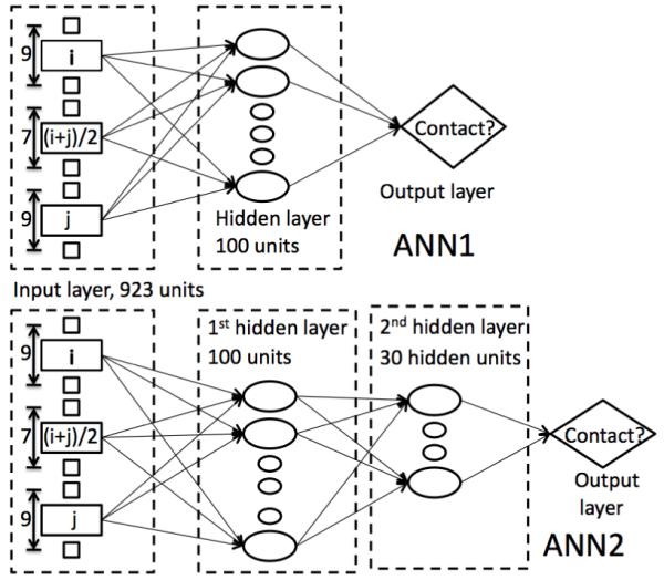
The neural-network architectures of ANN1 (Top) and ANN2 (Bottom).

Input for Networks

The overall input scheme is similar to that used in PROFcon¹⁴. There are three input windows: one central window and two residue windows (Fig. 1). The two residue windows correspond to target residues i and j. Residue windows have a window size of 9 residues as in PROFcon¹⁴. The central window is located at (i + j)/2. Trial and error determined a central window size of 7 residues. The following 34 input features are used for each residue in the above three windows: position specific scoring matrix (PSSM) from PSIBLAST²⁹ (20 values), representative amino acid properties (7 values) which are steric parameter, hydrophobicity, volume, polarizability, isoelectric point, helix probability and sheet probability^24,25,27, secondary structures [(1,0,0) for helix, (0,1,0) for strand, (0,0,1) for coil; 3 values. Here, (G,H,I) from the DSSP secondary-structure assignment program³⁰ are converted to H, (B,E) to E, and the rest to C], solvent accessibility [(1,0,0) for burying 75% or more of the maximum solvent accessible surface area, (0,1,0) for intermediate (25%-75%), (0,0,1) for exposed (<25%)], and one value for indicating terminal ends of protein sequences. In addition, there are 7 features that characterize the biophysical properties of residue pairs (hydrophobic-hydrophobic, polarpolar, charged-polar, opposite charged, same charged, aromatic-aromatic, and others¹⁴), and two binary features that characterize whether or not residues i and j are in low-complexity regions (SEG program^14,31). Furthermore, the following input features are used for connecting segment from i to j: 20 features for the composition of amino-acid residues, 3 inputs for the secondary structure composition, 1 input for the ratio of low complexity residues by SEG^14,31, and 11 inputs for the length of the segment (6, 7, 8, 9, 10 - 14, 15 - 19, 20 - 24, 25 - 29, 30 - 39, 40 - 49, and > 49)¹⁴. Finally, the global features include 20 global amino acid compositions, 3 secondary structure compositions, 1 for the ratio of low complexity region, and 4 inputs indicating the length of the sequence (1 - 61, 61 - 120, 121 - 240, and > 240)¹⁴. The total number of inputs for the neural network is 923 (including a bias) for a central window-size of 7 residues. Thus, the proposed network uses 185 additional features than PROFcon¹⁴. The additional features result from seven properties of amino acid residues, a three-state approximation for solvent accessibility, and a larger window size for the central window.

Secondary structures and accessible surface areas (ASA) from DSSP³⁰ are used in training and predicted values by SPINE²⁴ are used in testing and cross-validation. This arrangement was chosen because using predicted secondary structures for both training and testing lead to poorer results in solvent-accessibility prediction²⁵ and torsion angle prediction²⁷. All actual and predicted three-state secondary structures and ASA values are inputted as binary numbers. Three states for solvent accessibility are defined by taking 25% and 75% of the maximal value as the threshold values. Real-SPINE 3.0 is not used because the method was not available during the development of SPINE-2D. Moreover, the change in three-state accuracy of residue solvent accessibility is small from SPINE to Real-SPINE 3.0 and employing Real-SPINE 3.0 will unlikely make a significant change in the accuracy of SPINE-2D.

Performance evaluation

Our artificial neural network has only one output. Thus, one needs a threshold value to determine whether a contact is predicted. Here, we follow the practice used in CASP²¹ that employs a fixed number of top predictions such as top L, L/2, or L/5 predictions for a protein of sequence length L.

The performance of the proposed artificial neural network is mainly evaluated by accuracy and coverage. Accuracy (specificity) is the ratio of true positives (TP) to the number of predictions [the sum of true positives (TP) and false positives (FP)]. The coverage is the ratio of TP to the number of observed contacts [the sum of TP and false negatives (FN)]. We further monitor the change of accuracy as a function of the number of top predictions.

Dataset Construction and Usage

The main training dataset used in this paper originated from our previous 2640 non-homologous proteins for secondary structure prediction with the sequence identity less than 25%²⁴. This large dataset has 21.4% α-proteins, 10.8% β-proteins, and 67.6% other (mostly mixed α and β) proteins. We define α-proteins as proteins with more than 10% helical residues and less than 10% strand residues and β-proteins as those with more than 10% strand residues and less than 10% helical residues. The rest of the proteins in the database are defined as other proteins³². The above definition of all-alpha, all-beta proteins and other proteins is somewhat arbitrary. We use this definition to facilitate the prediction of structural classes based on predicted secondary structures and test our idea whether or not pre-classifying protein sequences in three structural categories would improve the accuracy of contact prediction (See discussion).

A dataset of 500 proteins is obtained from the 2640 protein dataset. It is obtained by randomly selecting proteins with chain length less than or equal to 400 residues. We restricted the chain length because training neural networks for contact prediction is a computationally intensive task. This 500-protein set contains 22.0% α proteins, 10.2% β proteins and 67.8% other proteins. The dataset is further divided randomly into 10 groups with 50 proteins each. Each time, nine groups are used for training and one group is used for independent testing. This procedure is repeated 10 times. During training, 5% of the training set is excluded from training and used as independent test to avoid possible over-training (overfit protection). That is, a ten-fold cross validation^33,34 is performed as in SPINE/Real-SPINE^24,25,27,26.

We further generate an additional independent dataset of 500 proteins with less than 400 residues in length from the remaining 2140 proteins of the original dataset. This set has 25.4% α proteins, 12.4% β proteins, and 62.2% other proteins, respectively.

We also apply our method to CASP 7 targets as an additional test¹. This dataset contains 89 proteins, with seven sequences (T290, T0346, T0359, T0340, T0366, T0315, T0317) whose sequence identity with the proteins in our training dataset is higher than 30%. Removing these seven sequences leads to a final dataset of 82 proteins.

Results

Table 1 reports ten-fold cross-validated accuracy and coverage by ANN1 and ANN2 among top L, L/2 and L/5 predictions. As expected, the full contact map is more accurately predicted (10% or more in accuracy) than the non-local contact map. However, the coverage (the fraction of predicted native contacts in all native contacts) is similar (the difference less than 2%). Thus, for a given protein, while more true positives are predicted in the full contact map than in the nonlocal contact map, this increase is balanced by the increase in the total number of true positives (native contacts). Less accurate prediction of nonlocal contacts is expected because of the lack of input features that can fully characterize nonlocal interactions.

Table 1.

Ten-fold cross-validated accuracy and coverage given by the single-hidden-layer (ANN1) and two-hidden-layer (ANN2) neural networks for predicting full-contact (|i - j| ≥ 6) and nonlocal contact (|i - j| ≥ 24) maps are compared at different number of top predictions (L, L/2, L/5). ANN2 is consistently more accurate than ANN1 (1-5% for full contact-map prediction and 0.3-1.6% for nonlocal contact-map prediction).

	Full Contact Mapa				Nonlocal Contact Mapb
	Accu.c		Cov.d		Accu.c		Cov.d
#e	ANN1	ANN2	ANN1	ANN2	ANN1	ANN2	ANN1	ANN2
L	27.4±1.3	29.1±1.1	15.5±0.8	16.0±0.6	14.8±0.8 (14.1±0.8f)	15.1±0.8 (14.4±0.8f)	13.5±1.5 (13.0±0.7f)	13.4±0.7 (12.7±0.7f)
L/2	34.6±1.6	37.3±1.8	9.8±0.5	10.3±0.5	17.1±1.4 (16.5±1.2f)	18.9±1.4 (18.5±1.4f)	8.4±1.1 (8.0±0.3f)	8.5±0.3 (8.1±0.3f)
L/5	42.2±2.1	47.2±2.2	5.1±0.3	5.3±0.5	22.6±2.0 (21.9±1.3f)	24.2±1.0 (23.8±1.0f)	3.7±0.7 (4.7±0.3f)	4.3±0.5 (4.1±0.5f)

^aAll residue-residue contacts with the separation of the sequence positions greater than or equal to 6.

^bNonlocal residue-residue contacts with the separation of the sequence positions greater than or equal to 24.

^cAccuracy: fraction of true positives in number of top predictions (L, L/2, or L/5).

^dCoverage: fraction of true positives in total number of native contacts.

^eThe number of predictions.

^fThe numbers in parentheses are ten-fold-cross-validated results by using the method trained for predicting the full contact map.

The second trend observed in Table 1 is that the accuracy improves significantly as the number of prediction is limited from top L, top L/2 to top L/5. For example, close to half (47%) of top L/5 predictions are correct for full contact map by ANN2. This compares to 37% and 29% for top L/2 and L predictions, respectively. Because top predictions are ranked by final prediction scores ranging from 0 to 1 (or -1 to 1 in ANN2), the above-described result indicates that the higher the prediction score, the more likely a predicted contact is a true native contact. Similar results were obtained in previous studies^9,14.

Table 1 further compares accuracy and coverage given by single-layer and two-layer neural networks. While there is a slight change for top L prediction, the accuracies in top L/2 and L/5 predictions improve by 2.7% and 5.0%, respectively, with a two-layer neural network. The improvement at top L/2 and L/5 predictions is statistically significant with a P-value of 0.04 based on the paired student-t test³⁵. There is no significant improvement in coverage, however.

The results described above are based on neural networks that are trained separately to predict full-contact and nonlocal contact maps. Table 1 also shows that predicting nonlocal contact maps by the method trained for full contact maps leads to a small but statistically significant (0.4-0.7%) reduction in accuracy and less significant change in coverage. Thus, specific training is useful for improving the accuracy of prediction.

Figure 2 provides a more detailed illustration of how the accuracy of prediction changes as a function of the number of top predictions (in unit of L). It is clear that ANN2 is consistently more accurate than ANN1 and their difference is larger as the number of predictions decreases. When the number of predictions is less than L, ANN2 is more accurate than ANN1 by 1 - 2% for non-local contact map and 2 - 5% for full contact map.

Figure 2.

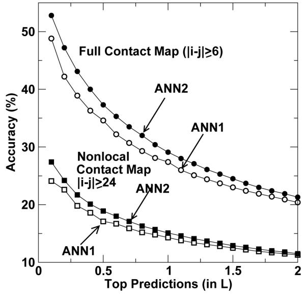
The accuracy of contact-map prediction as a function of the number of top predictions (in unit of protein sequence length L). Circles are for full contact-map (|i - j| ≥ 6), squares are for non-local contact-map (|i - j| ≥ 24) predictions. Open and filled symbols are by ANN1 and ANN2, respectively.

It is of interest to know the accuracy and coverage of contact prediction for proteins with different structural topologies (all α, all β, and other proteins) and different chain lengths (L < 120, 120 ≤ L ≤ 240, and L > 240). The ten-fold-cross-validated results given by ANN2 are shown in Table 2. These results indicate that β and other (mostly mixed α and β) proteins are predicted significantly more accurately (e.g. about 20% for top L/2 predictions of all contacts and 7-14% for top L/5 predictions of nonlocal contacts) than all α proteins while the coverage of the predictions for different structural proteins is essentially the same. Similar results were observed in previous studies^14,17.

Table 2.

Ten-fold cross-validated accuracy and coverage given by the two-hidden-layer (ANN2) neural networks for predicting full-contact (|i - j| ≥ 6) and nonlocal contact (|i - j| ≥ 24) maps at different number of top predictions (L, L/2, L/5) are shown for proteins of different structural classes (all α, all β and others) and different lengths (L < 120, 120 ≤ L ≤ 240, and L > 240).

		α	β	Other	L < 120	120 ≤ L ≤ 240	L > 240
Number of Proteins		110	52	338	154	214	132
Full Contact Mapsa
(L)	Accu.b	16.9	33.7	32.4	27.6	30.1	29.3
	Cov.c	17.1	14.4	15.9	20.1	15.2	12.5
(L/2)	Accu.b	22.0	41.8	41.8	35.1	38.4	38.2
	Cov.c	10.9	8.8	10.3	13.0	9.7	8.2
(L/5)	Accu.b	29.8	51.4	52.4	44.5	48.2	48.9
	Cov.c	5.9	4.3	5.3	7.0	4.9	4.2
Nonlocal C ontact Mapsd
(L)	Accu.b	9.4	14.1	17.1	13.5	16.3	15.0
	Cov.c	16.0	10.7	13.1	18.2	12.5	9.3
(L/2)	Accu.b	11.3	16.4	21.9	16.2	20.4	19.8
	Cov.c	10.3	6.3	8.3	11.5	7.8	6.1
(L/5)	Accu.b	13.8	20.4	28.2	19.7	25.5	27.1
	Cov.c	5.5	3.1	4.1	5.9	3.9	3.3

^aAll residue-residue contacts with the separation of the sequence positions greater than or equal to 6.

^bAccuracy: fraction of true positives in number of top predictions.

^cCoverage: fraction of true positives in total number of native contacts.

^dNonlocal residue-residue contacts with the separation of the sequence positions greater than or equal to 24.

Fig. 3 illustrates the change of prediction accuracy as a function of the number of top predictions. The overall trend is the same as what is observed in Table 2. Both full and nonlocal contact maps of helical proteins are predicted with the least accuracy.

Figure 3.

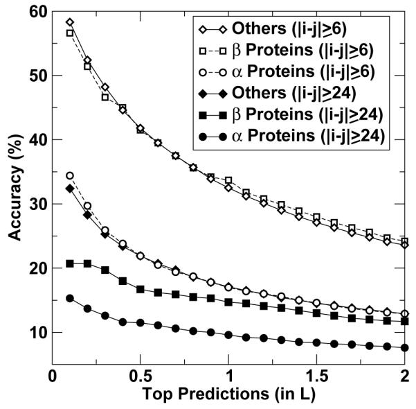
The accuracy of contact-map prediction as a function of the number of top predictions (in unit of protein sequence length L) for all α proteins (circles), all β proteins (squares) and others (triangles). Open and filled symbols are for full contact-map prediction (|i-j| ≥ 6) and non-local contact-map prediction with |i - j| ≥ 24, respectively.

Table 2 also shows that larger proteins are predicted with higher accuracy and lower coverage for the top L/5 predictions of full and nonlocal contacts. The accuracy of nonlocal-contact predictions (|i - j| ≥ 24) increases from 20%, 26% to 27% while the coverage decreases from 6%, 4% to 3% as protein lengths change from < 120, between 120 and 240, to > 240, respectively. Less accurate predictions for smaller proteins were also observed in previous studies¹⁴.

We show a more detailed distribution of prediction accuracy of full contact maps given by ANN2 for proteins of various structural topology and chain lengths in Fig. 4a and Fig. 4b, respectively. Almost all α proteins have prediction accuracy of 50% or less. On the other hand, the prediction accuracy of some β and other proteins can reach as high as 80%. The difference between proteins of different chain lengths, on the other hand, is not as significant (Fig. 4b).

Figure 4.

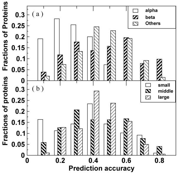
Distribution of prediction accuracy of the full contact map for (a) all α, all β, and other proteins and (b) proteins whose sequence lengths are less than 120, between 120 and 240 and larger than 240, respectively.

SPINE-2D is further tested on an independent test set of 500 proteins. The results are shown in Table 3. The difference between ten-fold cross-validated accuracy and independent test accuracy is between 1% to 1.6% for full-contact maps and 1.6-1.9% for nonlocal contact maps while the difference between coverages is between 0.2% and 1.6%. This suggests the overall accuracy and coverage from ten-fold-cross validation can be used to represent the overall accuracy of the method.

Table 3.

The ten-fold cross-validated accuracy and coverage given by the two-layer (ANN2) neural networks are compared to independent test results (Set 2 and CASP 7) at different number of top predictions (L, L/2, L/5). A consistent performance in different test sets is observed

	Full-contact mapa				Nonlocal contact mapb
	Accu.c		Cov.d		Accu.c			Cov.d
#e	Set 1f	Set 2g	Set 1f	Set 2g	Set 1f	Set 2g	CASP7h	Set 1f	Set 2g	CASP7h
L	29.1±1.1	27.7	16.0±0.6	15.7	15.1±0.8	13.5	-	13.4±0.7	11.8	-
L/2	37.3±1.8	35.8	10.3±0.5	10.1	18.9±1.4	17.0	-	8.5±0.3	7.5	-
L/5	47.2±2.2	45.6	5.3±0.5	5.3	24.2±1.0	22.5	25.9	4.3±0.5	3.8	4.5

^aAll residue-residue contacts with the separation of the sequence positions greater than or equal to 6.

^bNonlocal residue-residue contacts with the separation of the sequence positions greater than or equal to 24.

^cAccuracy: fraction of true positives in number of top predictions (L, L/2, or L/5).

^dCoverage: fraction of true positives in total number of native contacts.

^eThe number of predictions.

^fThe ten-fold cross validated result on the main dataset of 500 proteins

^gThe test result on the independent dataset of 500 proteins.

^h82 CASP 7 targets after removing 7 sequences whose sequence identities are greater than 30% with the training set of 500 proteins.

CASP 7 targets provide an additional test set¹. The average accuracy and coverage for the CASP 7 dataset is 25.9% for the accuracy and 4.5% for the coverage of predicted top L/5 nonlocal contacts (the official CASP assessment criterion) after removing seven sequences whose sequence identities are higher than 30% with the proteins in our training dataset. The accuracy and coverage are essentially unchanged with the full 89 protein set (26.3% and 4.2%, respectively). The accuracy and coverage are similar to the ten-fold-cross-validated accuracy of 24 ± 1% and coverage of 4.3±0.5%, respectively, (Table 3). This further illustrates the consistent accuracy and coverage by SPINE-2D.

DISCUSSION

In this paper, we developed a neural-network based method for predicting full and nonlocal contact maps. The ten-fold-cross-validated accuracies for top L, L/2 and L/5 predictions are 29%, 37%, and 47%, respectively, for full contact map, and 15%, 19% and 24%, respectively, for nonlocal contact maps. These accuracies are essentially unchanged when the methods are applied to an independent dataset of 500 proteins or CASP 7 targets.

It is not possible to make an exact comparison between the presented methods and other methods developed previously. Different methods have used different structural databases to train and were often tested by different datasets. Different test datasets likely have different compositions of all-α, all-β and other proteins. Because there are a significant difference (about 20% for full contact maps) between the prediction accuracy of all-α proteins and that of other proteins, varied compositions of a test dataset will lead to a different overall accuracy for the test set. It is perhaps more reasonable to compare the accuracy of all-α and all-β proteins given by different methods. For example, PROFcon¹⁴ reported an accuracy of 24% and a coverage of 11% for top L/2 full-contact predictions (sequence separation ≥6) in 131 all-α proteins and an accuracy of 35.0% and a coverage of 7.8% in 103 all-β proteins. The corresponding ten-fold-cross-validated accuracies (coverages) are 22.0% (10.9%) and 41.8% (8.8%), respectively, by SPINE-2D. This suggests that a significant improvement of accuracy in predicting β-protein contacts was achieved by SPINE-2D.

Nevertheless, the results predicted by several methods for CASP 7 targets can be directly compared to the results of SPINE-2D. We downloaded only the results of BETApro³⁶, PROFcon¹⁴, and SVMcon¹⁷ because the top L predictions for residue sequence separation of 6 or above are reported by these methods. We also include SAM-T06³⁷ in evaluating nonlocal contact predictions because it was one of the best predictors in CASP 7. We downloaded the results of 82 template-based modeling and free-modeling targets that are non-homologous to the SPINE-2D training set because the number of free-modeling targets (13) is too small to make a statistically significant assessment. We emphasize that this comparison only serves as an approximate guide because different methods have used different training sets, which may contain sequences homologous to CASP 7 targets (except SPINE-2D).

Table 4 compares top L/5 nonlocal contact predictions (|i - j| ≥ 24) given by several methods. The average accuracy of SPINE-2D is 26% that is 6% higher than the next best by BETApro. Here, the average accuracy is averaged over different number of target proteins. The accuracy of SPINE-2D does not change much if it is averaged over the same set of proteins reported by other methods. For example, the accuracy is 26.4% for averaging over the same 78 proteins reported by SAM-T06. Note a reduced number of proteins for other methods is either because these methods did not report results for some targets or because their reported predictions contain less than L/5 predictions of nonlocal contacts (|i - j| ≥ 24).

Table 4.

The accuracy and coverage of various contact-prediction methods in CASP 7 targets (both template-based and free-modeling targets) for top L/5 predictions of nonlocal contacts (|i - j| ≥ 24). This comparison serves as an approximate guide only because different methods have used different training sets which may contain sequences homologous to CASP 7 targets However, sequences of CASP 7 targets homologous to the SPINE-2D training set are removed. The number of targets for each method is different either because the method did not report the results for some proteins or because its reported predictions contain less than L/5 predictions of nonlocal contacts (|i - j| ≥ 24).

	BETAproa	PROFcona	SAM-T06a	SVMcona	SPINE-2D (ANN2)
No. b	62	62	78	78	82
Accu.c	20.0	13.7	15.2	16.6	25.9
Cov.d	3.3	5.1	4.1	2.9	4.5

^aPredictions are downloaded from CASP 7 website (http://predictioncenter.gc.ucdavis.edu/casp7/).

^bThe number of protein targets.

^cAccuracy.

^dCoverage.

To further compare SPINE-2D with other methods, we submit 50 testing proteins (one fold in our set) to SVMcon and PROFcon servers. The prediction accuracy is 21.5% by PROFcon, 26.5% by SVMcon, and 28.5% by SPINE-2D for top L full contact-map predictions while the coverage is 11.4% by PROFcon, 13.6% by SVMcon and 14.6% by SPINE-2D (ANN2). For top L/5 predictions of nonlocal contacts, the prediction accuracy is 18.5% by PROFcon, 21.6% by SVMcon, and 23.2% by SPINE-2D while the coverage is 3.9% by PROFcon, 3.5% by SVMcon and 3.4% by SPINE-2D (ANN2). Thus, SPINE-2D is among the most accurate prediction methods for contact maps.

It is observed in this and other studies^14,17 that there is a significant difference between the contact-prediction accuracy of all α proteins and that of other proteins (mixed α, β and all-β proteins). We speculate that nonlocal contacts between helices are more difficult to predict because unlike a single strand, a single helix (cylinder) has additional rotational degrees of freedom that can lead to more complex contact patterns. It is also known that helical residues are rarely mis-predicted to be strand residues and vice versa. Thus, three classes of all-α proteins, all β and other proteins can be predicted with high accuracy (91.5% by SPINE²⁴, for example). Consequently, it appears that a more accurate method would be obtained if neural-network predictors are trained separately for three structural classes of proteins. We tested this idea using the single-layer neural network and found that the improvement is insignificant, to our disappointment. Further studies are required to understand why predicted nonlocal contacts between all-α proteins are less accurate than those between all-β proteins and how to take advantage of this feature for more accurate contact predictions.

It is of interest to know if additional features introduced in this study are useful for improving the accuracy of prediction. We found that incorporation of seven physico-chemical features leads to about 2% increase in accuracy while a large central window yields an additional 0.5% improvement. However, using a three-state classification of ASA does not introduce a significant improvement over a two-state classification of ASA used in PROFcon¹⁴.

Another related question raised by this work is if the improvement from introducing a two-hidden-layer neural network is a result of more parameters (more neurons) or from a change in the network’s architecture. This question can be addressed by studying a single-hidden-layer neural network with more hidden neurons. We did not perform such a test on the contact map predictions because of computational time constraints. However, our unpublished tests during the development of Real-SPINE 3.0 indicates that incorporating more than 100 neurons in a single hidden layer does not produce any significant generalization power. On the other hand, introducing an additional hidden layer results in a significant improvement of the prediction accuracy of backbone dihedral angles. These results suggest that it is the change in the architecture of the neural network that is responsible for the improved accuracy. The introduction of a second-hidden-layer to the neural network allows for an additional processing level in it. This in turn allows for a better approximation of the nonlinear sequence-structure function of proteins.

References

- 1.Moult J, Fidelis K, Kryshtafovych A, Rost B, Hubbard T, Tramontano A. Critical assessment of methods of protein structure prediction-round VII. Proteins. 2007;69(Suppl 8):3–9. doi: 10.1002/prot.21767. [DOI] [PMC free article] [PubMed] [Google Scholar]
- 2.Vendruscolo M, Kussell E, Domany E. Recovery of protein structure from contact maps. Folding and Design. 1997;2:295–306. doi: 10.1016/S1359-0278(97)00041-2. [DOI] [PubMed] [Google Scholar]
- 3.Bonneau R, Ruczinski I, Tsai J, Baker D. Contact order and ab initio protein structure prediction. Protein Sci. 2002;11:1937–1944. doi: 10.1110/ps.3790102. [DOI] [PMC free article] [PubMed] [Google Scholar]
- 4.Goebel U, Sander C, Scheneider R, Valencia A. Correlated mutation and residue contacts in proteins. Proteins. 1994;18:309–317. doi: 10.1002/prot.340180402. [DOI] [PubMed] [Google Scholar]
- 5.Olmea O, Valencia A. Improving contact predictions by the combination of correlated mutations and other sources of sequence information. Folding and Design. 1997;2:s25–s32. doi: 10.1016/s1359-0278(97)00060-6. [DOI] [PubMed] [Google Scholar]
- 6.Hamilton N, Burrage K, Ragan M, Huber T. Protein contact prediction using patterns of correlation. Proteins. 2004;56:679–684. doi: 10.1002/prot.20160. [DOI] [PubMed] [Google Scholar]
- 7.Halperin I, Wolfson HJ, Nussinov R. Correlated mutations: advances and limitations. A study on fusion proteins and on the cohesion-dockerin families. Proteins. 2006;63:832–845. doi: 10.1002/prot.20933. [DOI] [PubMed] [Google Scholar]
- 8.Kundrotas PJ, Alexov EG. Predicting residue contacts using pragmatic correlated mutations method: reducing the false positives. BMC Bioinformatics. 2006;7:503. doi: 10.1186/1471-2105-7-503. [DOI] [PMC free article] [PubMed] [Google Scholar]
- 9.Fariselli P, Casadio R. A neural network based predictor of residue contacts in proteins. Protein Engineering. 1999;12:15–21. doi: 10.1093/protein/12.1.15. [DOI] [PubMed] [Google Scholar]
- 10.Fariselli P, Olmea O, Valencia A, Casadio R. Progress in predicting inter-residue contacts of proteins with neural networks and correlated mutations. Proteins. 2001;(Suppl 5):157–162. doi: 10.1002/prot.1173. [DOI] [PubMed] [Google Scholar]
- 11.Pollastri G, Baldi P, Fariselli P, Casadio R. Improved prediction of the number of residue contacts in proteins by recurrent neural networks. Bioinformatics. 2001;17:s234–s242. doi: 10.1093/bioinformatics/17.suppl_1.s234. [DOI] [PubMed] [Google Scholar]
- 12.Pollastri G, Baldi P. Prediction of contact maps by GIOHMMs and recurrent neural networks using lateral propagation from all four cardinal corners. Bioinformatics. 2002;18:s62–s70. doi: 10.1093/bioinformatics/18.suppl_1.s62. [DOI] [PubMed] [Google Scholar]
- 13.Zhang G, Huang DS. Prediction of inter-residue contacts map based on genetic algorithm optimized radial basis function neural network and binary input encoding scheme. J. Comput-Aided Mole. Des. 2004;18:797–810. doi: 10.1007/s10822-005-0578-7. [DOI] [PubMed] [Google Scholar]
- 14.Punta M, Rost B. PROFcon: novel prediction of long-range contacts. Bioinformatics. 2005;21:2960–2968. doi: 10.1093/bioinformatics/bti454. [DOI] [PubMed] [Google Scholar]
- 15.Walsh Vullo IA., Pollastri G. A two-stage approach from improved prediction of residue contact maps. BMC Bioinformatics. 2006;7:180. doi: 10.1186/1471-2105-7-180. [DOI] [PMC free article] [PubMed] [Google Scholar]
- 16.Zhao Y, Karypis G. Prediction of contact maps using support vector machines; Proc of the IEEE Symposium on Bioinformatics and BioEngineering; 2003.pp. 26–36. [Google Scholar]
- 17.Cheng J, Baldi P. Improved residue contact prediction using support vector machines and a large feature set. BMC Bioinformatics. 2007;8:113. doi: 10.1186/1471-2105-8-113. [DOI] [PMC free article] [PubMed] [Google Scholar]
- 18.Shao Y, Bystroff C. Predicting interresidue contacts using templates and pathways. Proteins. 2003;53:497–502. doi: 10.1002/prot.10539. [DOI] [PubMed] [Google Scholar]
- 19.Maccallum RM. Striped sheets and protein contact prediction. Bioinformatics. 2004;20(1):224–231. doi: 10.1093/bioinformatics/bth913. [DOI] [PubMed] [Google Scholar]
- 20.Mangal Gupta NN., Biswas S. Evolution and similarity evaluation of protein structures in contact map space. Proteins. 2005;59:196–204. doi: 10.1002/prot.20415. [DOI] [PubMed] [Google Scholar]
- 21.Izarzugaza J, Grana O, Tress M, Valencia A, Clarke N. Assessment of intermolecular contact prediction for CASP7. Proteins. 2007;69(Suppl):152–158. doi: 10.1002/prot.21637. [DOI] [PubMed] [Google Scholar]
- 22.Miller C, Eisenberg D. Using inferred residue contacts to distinguish between correct and incorrect protein models. Bioinformatics. 2008;24:1575–1582. doi: 10.1093/bioinformatics/btn248. [DOI] [PMC free article] [PubMed] [Google Scholar]
- 23.Zhang Y, Kolinski A, Skolnick J. TOUCHSTONE II: a new approach to ab initio protein structure prediction. Biophys J. 2003;85:1145–1164. doi: 10.1016/S0006-3495(03)74551-2. [DOI] [PMC free article] [PubMed] [Google Scholar]
- 24.Dor O, Zhou Y. Achieving 80% ten-fold cross-validated accuracy for secondary structure prediction by large-scale training. Proteins. 2007;66:838–845. doi: 10.1002/prot.21298. [DOI] [PubMed] [Google Scholar]
- 25.Dor O, Zhou Y. Real-SPINE: An integrated system of neural networks for real-value prediction of protein structural properties. Proteins. 2007;68:76–81. doi: 10.1002/prot.21408. [DOI] [PubMed] [Google Scholar]
- 26.Faraggi E, Xue B, Zhou Y. Improving the accuracy of predicting real-value backbone torsion angles and residue solvent accessibility by guided learning through two-layer neural networks. Proteins. 2008 doi: 10.1002/prot.22193. in press. [DOI] [PMC free article] [PubMed] [Google Scholar]
- 27.Xue B, Dor O, Faraggi E, Zhou Y. Real-value prediction of backbone torsion angles. Proteins. 2008;72:427–433. doi: 10.1002/prot.21940. [DOI] [PubMed] [Google Scholar]
- 28.Zupan J. Introduction to artificial neural network (ANN) methods: what they are and how to use them. Acta Chimica Slovenica. 1994;41:327–352. [Google Scholar]
- 29.Altschul S, Madden T, Schaffer A, Zhang Zhang ZJ., Miller W, Lipman D. Gapped BLAST and PSI-BLAST: a new generation of protein database search programs. Nucl. Aci. Res. 1997;25:3389–3402. doi: 10.1093/nar/25.17.3389. [DOI] [PMC free article] [PubMed] [Google Scholar]
- 30.Kabsch W, Sander C. Dictionary of protein secondary structure: pattern recognition of hydrogen-bonded and geometrical features. Biopolymers. 1983;22:2577–2637. doi: 10.1002/bip.360221211. [DOI] [PubMed] [Google Scholar]
- 31.Wootton J, Federhen S. Analysis of compositionally biased regions in sequence databases. Meth. Enzymol. 1996;266:554–571. doi: 10.1016/s0076-6879(96)66035-2. [DOI] [PubMed] [Google Scholar]
- 32.Zhang C, Liu S, Zhou H, Zhou Y. The dependence of all-atom statistical potentials on training structural database. Biophys. J. 2004;86:3349–3358. doi: 10.1529/biophysj.103.035998. [DOI] [PMC free article] [PubMed] [Google Scholar]
- 33.Riis S, Kroph A. Improving prediction of protein secondary structure using structured neural networks and multiple sequence alignments. J. Comput. Biol. 1996;3:163–183. doi: 10.1089/cmb.1996.3.163. [DOI] [PubMed] [Google Scholar]
- 34.Sim J, Kim S, Lee J. Pprodo: Prediction of protein domain boundaries using neural networks. Proteins: Struct. Funct. Bioinfo. 2005;59:627–632. doi: 10.1002/prot.20442. [DOI] [PubMed] [Google Scholar]
- 35.GraphPad Software http://www.graphpad.com/quickcalcs/ttest1.cfm.
- 36.Cheng J, Baldi P. Three-stage prediction of protein β-sheets by neural networks, alignmentsand graph algorithms. Bioinformatics. 2005;21(Suppl):i75–i84. doi: 10.1093/bioinformatics/bti1004. [DOI] [PubMed] [Google Scholar]
- 37.Shackleford G, Karplus K. Contact prediction using mutual information and neural nets. Proteins. 2007;69(S8):159–164. doi: 10.1002/prot.21791. [DOI] [PubMed] [Google Scholar]