

Abstract
To explore the multivariate nature of fMRI data and to consider the inter-subject brain response discrepancies, a multivariate and brain response model-free method is fundamentally required. Two such methods are presented in this paper by integrating a machine learning algorithm, the support vector machine (SVM), and the random effect model. Without any brain response modeling, SVM was used to extract a whole brain spatial discriminance map (SDM), representing the brain response difference between the contrasted experimental conditions. Population inference was then obtained through the random effect analysis (RFX) or permutation testing (PMU) on the individual subjects’ SDMs. Applied to arterial spin labeling (ASL) perfusion fMRI data, SDM RFX yielded lower false-positive rates in the null hypothesis test and higher detection sensitivity for synthetic activations with varying cluster size and activation strengths, compared to the univariate general linear model (GLM) based RFX. For a sensory-motor ASL fMRI study, both SDM RFX and SDM PMU yielded similar activation patterns to GLM RFX and GLM PMU, respectively, but with higher t values and cluster extensions at the same significance level. Capitalizing on the absence of temporal noise correlation in ASL data, this study also incorporated PMU in the individual level GLM and SVM analysis accompanied by group level analysis through RFX or group level PMU. Providing inferences on the probability of being activated or deactivated at each voxel, these individual level PMU based group analysis methods can be used to threshold the analysis results of GLM RFX, SDM RFX or SDM PMU.
Keywords: group analysis, random effect analysis, support vector machine, ASL perfusion fMRI, permutation testing
Introduction
Functional MRI has been a standard tool for visualizing regional brain activations during sensorimotor or cognitive tasks. fMRI data are widely processed using a general linear model (GLM) based approach, in which fMRI time series data are fitted to an a priori defined reference function; the fitting parameters are then contrasted to produce a test statistic at each voxel(Bandettini et al., 1993; Friston et al., 1995b,c; Worsley and Friston, 1995). Assuming linear brain responses to the functional stimuli and modeling each voxel’s time series with a canonical hemodynamic response function (HRF) (Friston et al., 1994; Hopfinger et al., 2000), this univariate GLM approach may by suboptimal for fMRI data analysis for the following two reasons. First, by treating each voxel’s time series as an independent event, it ignores the abundant spatial correlations of fMRI data, so that it can not take advantage of the fact that several brain regions may respond to the same functional stimuli simultaneously. Although spatial smoothing can partly take the spatial correlations into account, it can only consider those existing in a constrained neighborhood. Moreover, it could worsen sensitivity by smoothing in incoherent signal. A multivariate method is fundamentally required to discover coherent but spatially distributed brain activations. Given the consistency assumption of the target brain activations along the time, which is a basic premise of fMRI, potential sensitivity improvement could be achieved by searching the activation pattern as a unit instead of doing it independently in each voxel. While this is useful for any kind of fMRI study, it is particularly beneficial for a weak signal detection as in arterial spin labeling (ASL) perfusion fMRI (Detre et al., 1992), which suffers from relatively low sensitivity (Buxton, 2002) due to the low SNR (Wong, 1999). Second, the brain response may be nonlinear to the functional stimuli and the actual shape of the HRF may differ significantly from the canonical one in different subject populations or from voxel to voxel (Aguirre et al., 1998). To consider the HRF discrepancies, a HRF model-free approach is highly preferred for fMRI data analysis.
Several multivariate methods have been used in fMRI data analysis over the last decade, including principal component analysis (PCA) (Friston et al., 1993; Bullmore et al., 1996), partial least square (PLS) (McIntosha et al., 1996), canonical variate analysis (CVA) (Friston et al., 1995a; Worsley et al., 1997), and independent component analysis (ICA) (McKeown and Sejnowski, 1998). While PCA and ICA are purely data-driven, they both present difficulties of interpreting the extracted components, identifying the number of interested components, and performing group analyses. PLS and CVA provide advantages of data dimension reduction and for incorporating a priori information such as the experiment design function or task performance. While using the prior information can alleviate some the difficulties of PCA decomposed component identification and interpretation, it is still based on the assumption that the measured effects are linearly related to the regressors in the design matrix as in the standard univariate GLM approach. Additionally, the extracted maximal effects may not correspond to the a priori expectations for the functional study, since both PLS and CVA are based on PCA decomposition, which depends only on the data variance.
Support vector machine (SVM) (Vapnik, 1995; Burges, 1998) is a data classification algorithm, that has been increasingly employed as a multivariate method in BOLD fMRI for brain response prediction and classification (Cox and Savoy, 2003; Wang et al., 2003a; Mitchell et al., 2004; Davatzikos et al., 2005; LaConte et al., 2005; Mourão-Miranda et al., 2005). In contrast to the multivariate methods described above, SVM can extract a unique brain discrepancy map which is directly related to the measured effect difference between different experimental brain conditions (LaConte et al., 2005; Mourão-Miranda et al., 2005). To differentiate this approach from statistical parametric mapping (SPM) (Friston, 1996), this kind of discrepancy map has been termed “spatial discriminance map” (SDM) in this paper. While this approach can reveal coherent brain activations for individual subjects, a statistical framework is required for a population level inference on the significance of the detected discriminance. A multi-subject level SDM extraction with a statistic inference approach has previously been proposed by Mourão-Miranda et al. (Mourão-Miranda et al., 2005). Similar to the “fixed effect model” based group fMRI data analysis (Penny et al., 2003), this approach was designed for concatenated multi-subject data, and the associated multi-subject SDM only represents the brain discriminance between different states for the specific subjects included in the experiment. Therefore it still cannot provide a population inference on the brain descriminance. Additionally, part of the discriminance represented by the multi-subject SDM may be contributed by anatomical differences between different subjects due to direct data concatenation.
To provide a population inference on the spatial discriminance, we used both random effects analysis (RFX) (Penny et al., 2003) and permutation testing (PMU) (Nichols and Holmes, 2002) to assess the between-subject variability of the brain activation revealed by individual SDMs. Correspondingly, two SVM based fMRI data group analysis methods were presented: 1) individual level SDM extraction with RFX based group analysis (SDM RFX) and 2) individual level SDM extraction with PMU based group analysis (SDM PMU). A linear SVM (Burges, 1998) was used to extract the individual level SDMs using similar preprocessing approaches reported in (LaConte et al., 2005; Mourão-Miranda et al., 2005). Null-hypothesis resting ASL perfusion MR data and synthetic functional activations with variable cluster size and activation strength were also used to validate the proposed methods.
Since ASL perfusion signal is devoid of temporally autocorrelated noise (Aguirre et al., 2002), PMU (Nichols and Holmes, 2002) is also directly applicable to individual subject ASL perfusion data analysis. Combining individual level permutation based GLM and group level RFX or PMU, this paper also presents several other group analysis methods for ASL perfusion fMRI. All proposed methods, SDM RFX, SDM PMU, and the individual level SDM or GLM permutation testing based group analysis, are finally applied to a sensory-motor task ASL perfusion fMRI dataset.
Theory
Data reduction
In a typical fMRI scan, an image volume usually contains thousands of voxels, resulting in a very large spatial dimension of the fMRI data. For example, a 64 × 64 × 12 ASL perfusion volume may have approximately 30, 000 within-brain voxels. Training an SVM classifier for vectors with such a high dimension is quite computationally intensive, possibly even unmanageable for current computers. Therefore, data reduction is mandatory for SVM classification on fMRI data. A widely used multi-dimensional data reduction method is principal component analysis (PCA) (Vetterling and Flannery, 2002). Decomposing the original fMRI data into a set of principal vectors (eigenvectors sorted by their corresponding eigenvalues) and an associated principal component set, an optimal dimensionality reduction can be achieved by representing the original data with these principal vectors (Vetterling and Flannery, 2002). However, direct PCA decomposition is generally nontrivial due to the large spatial dimension of fMRI data. An alternative approach for a moderate data set is to estimate the principal vectors from the PCA decomposition along the temporal dimension (Friston et al., 1995a; Mourão-Miranda et al., 2005; Wang et al., 2006), since the temporal dimension is usually much smaller than the spatial dimension. When the number of images increases, or the number of subjects increases in the case of multi-subject classification, the whole data size may be too large to be loaded into computer’s memory. Instead of conventional PCA, a cascade recursive least squared network based PCA (CRLS-PCA) (Cichocki et al., 1996; Wang et al., 2003b, 2005c, 2006) can be used to extract the principal vectors sequentially.
Suppose we have an fMRI data matrix SN×L with one volume per column and one voxel per row. Here N and L are the number of within brain voxels and the number of timepoints, N≫L. Since S only has L nonzero eigenvalue associated principal vectors (eigenvectors) E = (e1, e2,⋯, eL), ei = (ei,1, ei,2,⋯, ei,N)T (Vetterling and Flannery, 2002), after PCA decomposition, S can be losslessly compressed into a L × L matrix X = ETS, with one representation coefficient vector xi = (x1,i, x2,i,…, xL,i)T per column corresponding to one original image volume. These coefficient vector series X = (x1, x2,⋯, xL) are fed to the SVM training process as described below.
Linear support vector machine
Consider the two class problem and label the dimension reduced data as {xi, yi}, i = 1,⋯, L, yi ∈ {−1, +1} (−1 indicates condition A, +1 indicates condition B), a linear SVM as illustrated by Fig. 1 seeks a hyperplane w · x + b = 0 in the feature space ℝL with the largest margin separating the coefficient vectors with label +1 from those with label −1. Here, w is the weight vector normal to the hyperplane, and ||w|| is the Euclidean norm of w. b is the offset, and |b|/||w|| is the perpendicular distance from the hyperplane to the origin.
Figure 1.

Illustration of a separating hyperplane (solid line) with a maximal margin determined by a linear SVM. Dashed lines are the boundary hyperplanes of the separated classes and the circled symbols are the support vectors.
Using Lagrangian multiplier method, the solution can be found as (Burges, 1998):
| (1) |
where α ≥0 is the Lagrangian multiplier, which is constrained by Σiαiyi = 0. The points with α > 0 are called “support vectors”, which lie in the supporting hyperplanes. For any other points, α = 0.
Spatial discriminance map
For linear SVM, the separating hyperplane is uniquely defined by the normal weight w in Eq. 1, which represents the direction along which the training samples of both classes differ most. A spatial discriminance map (SDM) (also called “discriminating volume” in (Mourão-Miranda et al., 2005)) can be also obtained by mapping w back to the original image space through:
| (2) |
The positive value of SDM means higher activation during the task B than task A; negative value means lower activation during task B than task A. Since each training sample (for fMRI, a sample is an image volume) is treated as a unit, the spatial correlations within fMRI data are inherently explored during the SVM classifier training by affecting the direction therefore affecting the spatial patterns of the extracted SDM, so that SDM provides a way to explore the spatially coherent activations.
SDM RFX
So far, only the individual level brain state discriminance was considered. To provide a population inference on the detected discriminance, a “random effect model” (Penny et al., 2003) can be used to consider the between-subject variability of the spatial discriminance. Following the “summary statistic” (Friston and Pocock, 1992; Holmes and Friston, 1998) approach, a random effect analysis (RFX) of the individual level SDM can be performed using a one-sample t-test. This represents the first SVM-based fMRI data group analysis method proposed in this paper: SDM RFX.
Permutation testing
Permutation testing (Nichols and Holmes, 2002) was also used to assess the population level statistical inference on the detected discriminance in the second SVM-based group analysis method: SDM PMU. The significance of discriminance is assessed by calculating a probability map through randomly permuting the sign of individual SDMs and performing a one-sample t-test for each sign flipping.
Due to the absence of temporal noise correlation in ASL perfusion image series (Aguirre et al., 2002), PMU is also directly applicable to the individual SDM estimation process or the individual level GLM analysis for ASL fMRI data. While PMU can be used to assess the significance of individual SDM (Mourão-Miranda et al., 2005) or GLM results (Aguirre et al., 2003), it can be also used to form an ASL perfusion fMRI group analysis. For each individual SDM, a P map was first calculated using PMU. To indicate the discriminance direction, the P map was set to positive or negative according to the sign of SDM value at each voxel. To facilitate signal intensity interpretation, a new map, named reversed P map (rPM), was also generated from the P map by keeping the sign but subtracting the absolute value from 1. Similar procedures were also performed for individual level GLM analysis to calculate an rPM. The rPMs for SDMs and GLM parametric maps were abbreviated as SDMrPM and GLMrPM, respectively. Similar to SDM RFX and SDM PMU, group analysis methods can be then formed by RFX or PMU on the individual SDMrPM or GLMrPM. Since an rPM is generated from the individual level PMU, it should be less sensitive to noise, outliers, and subject related response strength variations, therefore should be more consistent across subjects than SDM or GLM parametric map. Consequently, individual rPMs based group analysis could increase the detection sensitivity as compared to group analysis based on individual SDM or individual GLM parametric maps. However, the individual rPMs based group analysis methods cannot provide inference on the activation or deactivation strength, but rather only on the probability of activation or deactivation regardless of their strength. This provides another perspective to view the data, and can be also used to threshold the individual SDM or individual GLM parametric map based group analysis results.
As a summary, Fig. 2 illustrates a basic paradigm of SVM-based fMRI data analysis procedures, containing 4 major steps: data preprocessing, dimension reduction, SDM and SDMrPM calculation and group level analysis through one-sample t-test or permutation testing. The data preprocessing step contains motion correction, coregistration, smoothing, cerebral blood flow (CBF) image calculation (only required for ASL perfusion fMRI) and spatial normalization. The same paradigm works for GLM based approaches by replacing SVM with GLM and SDM with GLM parametric map in Fig. 2.
Figure 2.

Diagram of individual SVM classification with or without permutation testing based group analysis. All subjects’ functional images were properly preprocessed and only the within voxels were considered. L, S, E, and X are the number of images per subject, original functional data matrix, decomposition matrix consisting of eigen vectors of S, and representing coefficients matrix respectively.
Materials and methods
Imaging parameters
Imaging experiments were performed on a 3T Siemens Trio whole body MR scanner with a standard transmit/receive (Tx/Rx) head coil (Bruker BioSpin, USA). An amplitude modulated CASL perfusion imaging sequence optimized for 3.0T was used for perfusion fMRI scans (Wang et al., 2005b) with parameters of: labeling time = 1.6 sec, post-labeling delay = 800 ms, field-of-view (FOV)=22cm, matrix=64×64×12, bandwidth=3kHz/pixel, flip angle=90°, TR=3sec TE=17, slice thickness 7 mm, inter-slice space 1.25 mm.
High resolution 3D T1-weighted anatomical images using the MPRAGE (TR/TE/TI = 1630/3/1100msec) sequence were additionally obtained for each subject for spatial image normalization.
Resting and sensory-motor task ASL perfusion MR scan
Written informed consent was obtained from each subject before scanning following an Institutional Review Board approved protocol for the associated experiments. Seven normal subjects lying in the scanner at rest were scanned for 6 mins using the CASL sequence mentioned above, resulting in 60 control/label image pairs. Another 10 normal subjects were scanned for 7.2 mins performing a self-paced right hand fingertapping task when they saw the visual stimuli on the screen. A block design was used, consisting of 3 task blocks separating by a baseline block. Each block lasts for 1.2 min. The visual stimuli during the task state was an 8 Hz reversing black and white checkerboard. 72 control/label image pairs were obtained for each subject.
Data preprocessing
The resting images (60 control/label pairs) and the functional images (72 control/label pairs) of each subject were motion corrected, coregistered with the T1 images, and smoothed with an isotropic Gaussian filter (FWHM=8 mm) using the SPM2 software (Wellcome Department of Cognitive Neurology, London, UK, http://www.fil.ion.ucl.ac.uk). The perfusion weighted images were calculated by pair-wise subtraction of the label/control image pairs. The quantitative CBF images were calculated using the method given in (Wang et al., 2005b). The T1 image was normalized to the Montreal Neurological Institute/International Consortium for Brain Mapping (MNI/ICBM) 152 standard brain using SPM2, the same normalization parameters were also used to map the CBF images to the MNI/ICBM standard space.
Dimension reduction
A mask generated from the raw (EPI) images was used to remove the out-of-brain voxels to reduce the computational burden. Each spatially normalized CBF image (without the out-of-brain voxels) was then reformatted into a column vector. After mean centering and grand mean normalization using each subject’s global CBF value, standard singular vector decomposition (SVD) (Press et al., 2002) was used to calculate all nonzero eigenvalue associated eigenvectors along the time dimension of the fMRI data matrix (each column is an image vector). Each image vector was finally projected into the eigen space spanned by the extracted eigenvectors, yielding a representing coefficient vector.
Null hypothesis test and synthetic brain activations
The resting ASL perfusion image series were used to evaluate SDM RFX under the null hypothesis that there is no activation carried in the image series. The resting image series were randomly permuted and two brain states, baseline and task, were assumed to be invoked during the scan, with 3 repetitions, each consisting of 10 baseline images and 10 task images. The average temporal SNR of the null hypothesis data was greater than 8 for every subject. PCA data reduction, data representations and SVM training were then performed the same as for the activation data analysis. With the same permuted time series and the same block wise task paradigm, voxel based GLM RFX was also performed as a comparison.
Artificial activations were inserted into the same permuted spatially normalized resting CBF image series as described above. Two separate regions in the grey matter were chosen to simulate distant spatial correlations. To simulate the neighboring spatial correlations, 5 different clusters for the two regions were used with 6, 10, 16, 24, 32 voxels with (2,4), (4,6), (6,10), (10,14), (14,18) for region 1 and region 2 respectively. For each cluster simulation, 5 different artificial activations were synthesized with a mean 2, 5, 10, 15 and 20 percent CBF signal changes based on the baseline CBF values, resulting in 25 total simulations. Random variations of the mean signal change strength were also introduced to simulate the between-subject response variability. The simulated functional CBF image series were then processed through data reduction, SVM training, SDM calculation and SDM RFX as shown in Fig. 2. Voxel based GLM RFX was conducted as a comparison for the activation data. For each simulation, the mean t value within the regions used for inserting artificial activations was calculated from the t map of GLM RFX and SDM RFX.
ROC analysis
The receiver operator characteristic (ROC) method (Metz, 1978) was further used to assess the performance and efficacy of SVM based fMRI data analysis method. Without referring to the statistical significance of the result, ROC provides an easy tool for methodological performance comparison. Two ROIs located in the grey matter were used to insert the synthetic activations into the null-hypothesis CBF images as described above. The first ROI consists of 113 voxels and the second ROI consists of 49 voxels. Both ROIs were larger than those used in the above evaluations to allow an enough range for the true positive rate (TPR). Two series of synthetic data were generated using the same pseudo-task paradigm as stated above and inserting artificial activations into the first ROI and both ROIs with a 1, 2, 5, 10, 20, 40 percent signal changes based on the baseline CBF, resulting in totally 12 data sets. These synthetic data were then analyzed with the univariate GLM approach and the SVM based approach.
To calculate the ROC curves, each subject’s GLM parametric map and SDM were sorted in descending order. ROC curves were generated based on the true positive (activation) rate vs. the false positive (activation) rate throughout the range of sorted maps, by comparing the locations of the predetermined ROIs. The same process was conducted for the t maps of GLM RFX and SDM RFX. The area under curve (AUC) was used as the surrogate score for the efficacy of each method.
Stability test of SDM extraction
36 experiments were conducted to test the stability of SDM extraction. In each case, one image from the baseline condition and one image from the task condition were pseudo-randomly excluded, and an SDM was extracted from the rest of functional images using the method described above. A correlation coefficient was then calculated between this SDM and the one from the whole dataset to measure the variations of SDM extractions. The same experiments were repeated for all 10 subjects who participated in the sensorimotor fMRI scan. Since the vast majority of voxels in SDM could be close to zero, the correlation between two SDMs could be high even the interested activation regions are markedly different. To further verify the stability of SDM extraction for the hypothesized activation regions, the same stability evaluations were performed by checking the corrections just within the activation regions. The regions were defined by the suprathresholded activation clusters using SDM RFX with an uncorrected P < 0.001.
Individual SDM and multi-subject SDM extraction
SVMlight software (Joachim, 1999) was used to train a linear SVM classifier and extract the individual SDM in this paper. The source code of this software was modified to allow reading binary image representation coefficients, permutation operations and calculating SDMs and SDMrPM. For calculating SDMrPM, the class labels assigned to all functional images were permuted 2001 times instead of permuting CBF data series directly, and 2001 SDMs were subsequently calculated using SVMlight. The “fixed effect model” based multi-subject SDM (Mourão-Miranda et al., 2005) was also extracted as a comparison. All subjects’ CBF images were first concatenated and dimension reduced using the same PCA based data reduction step described above. The representing coefficient vectors were then subjected to the SVM classification to extract a multi-subject SDM as did in (Mourão-Miranda et al., 2005). A P map was also generated from 2001 permutations to assess the significance of the multi-subject SDM.
The leave-one-out test (Allen, 1974) was used to validate the performance of the trained multi-subject SVM classifier for predicting the status of any image from any subject. During the prediction experiment, the eigen vectors were still extracted from all subjects, all images were subsequently projected to the eigen space as stated above. The only difference is that images from one subject were not fed into the training process but rather fed into the prediction process.
Due to the extremely long computation time required by the individual level permutation based group analyses, SDMrPM and GLMrPM based group analysis, were only conducted for the sensory-motor task functional data. The total 2001 + 2001 × 10 × 2 SVM jobs were automatically distributed to a cluster of 20 computers using the VoxBo job engine (http://voxbo.org). SDMs and SDMrPMs were calculated using in-house software written in C language. SDM RFX and SDMrPM RFX, were then performed using SPM2 software. The group level permutation testing (in SDM PMU and GLM PMU) was performed using the SnPM3 software (http://www.sph.umich.edu/ni-stat/SnPM/).
GLM RFX, GLM PMU and GLMrPM RFX
The univariate GLM-based analysis was performed using SPM2 software. Population inferences were conducted through one-sample t-test (GLM RFX) or the group level PMU (GLM PMU) based on the individual GLM parametric maps using the “random effect model” (Holmes and Friston, 1998; Penny et al., 2003; Brett et al., 2003). GLM RFX was applied to the null-hypothesis data, synthetic functional data and the sensory-motor task fMRI data. GLM PMU and GLMrPM RFX were only applied to the sensory-motor task fMRI data due to the huge computational burden of the permutation testing if applied to the synthetic data. The reference function assigned to all functional images were randomly permuted 2001 times. After 2001 GLM analyses, a GLMrPM was calculated from the 2001 GLM parametric maps. Group level analyses were then performed using one-sample t-test or PMU.
Results
SDM RFX for the null hypothesis data and synthetic functional data
Fig. 3 and Fig. 4 are the suprathresholded t maps of GLM RFX and SDM RFX from the null hypothesis resting CBF image series. With the same threshold abs(t) > 3 (corresponding to P < 0.012), GLM RFX yielded many falsely detected activated voxels, while SDM RFX did not show any suprathresholded voxels.
Figure 3.

GLM RFX results of the null hypothesis resting CBF data. The t threshold is arbitrarily chosen to be 3.
Figure 4.
SDM RFX results of the null hypothesis resting CBF data. The t threshold is the same as in Fig. 3.
Fig. 5 shows the mean t values of GLM RFX and SDM RFX from the simulated functional CBF image series within the a priori two regions for inserting artificial activations. Both GLM RFX and SDM RFX demonstrated increased mean t values when the signal change magnitude increased. For any cluster size and for every signal change strength, SDM RFX yielded a higher mean t value than GLM RFX.
Figure 5.

Mean t values of the group analysis t maps of GLM RFX and SDM RFX for all simulations.
ROC analysis
Fig. 6 shows the ROC analyses results of GLM and SVM based data analyses on various synthetic ASL perfusion fMRI data. Fig. 6A is the ROC curve of the GLM and SVM based data analyses on a representative subject’s synthetic data generated with the 113 voxels ROI and 5 percent signal change. For this subject, SVM clearly demonstrated better sensitivity and less FPR than GLM. Fig. 6B shows the mean AUC of ROC curves of GLM and SVM on the synthetic data. For simulations with both clusters, SVM yielded increased AUC for activation strength from 2 to 20 percent of signal change compared to GLM. For cluster size 2 (using both the 113 voxels ROI and the 49 voxels ROI), SVM presented significant AUC increase at 2 (P < 0.05, paired t-test) and 5 (P < 0.02, paired t-test) percent of signal change. At the group level as shown in Fig. 6C, for all synthetic data using the same a prior ROI, SDM RFX yielded increased AUC for every simulated percent of signal change, compared to GLM RFX.
Figure 6.

ROC analysis results. A) ROC curves of the GLM parametric map and the SDM of a representative subject’s synthetic data. The artificial activations were inserted into one ROI of 113 voxels with 5 percent of signal change. B) averaged (7 subjects) AUCs of GLM and SDM based analyses on the synthetic functional data with various percentage signal changes within two ROIs. The error bars mean the standard deviations. C) AUCs of the GLM RFX and SDM RFX on the same synthetic data as in B).
Stability test of SDM extraction
The SDM stability evaluation results are shown in Fig. 7. By randomly excluding an image from the baseline and the task condition, the SDM extracted from the rest of the dataset was significantly (P < 0.00001) highly correlated (mean r > 0.975) to the SDM from the whole dataset for every subject (Fig. 7A). As shown in Fig. 7B, the stability of SDM values within the hypothesized activation regions were even better (mean r > 0.986, P < 0.0005).
Figure 7.

SDM extraction variations A) of the whole brain, B) within the hypothesized activation regions illustrated by the correlation coefficient between the SDM of the whole dataset and the SDM of a new dataset after randomly excluding an image from the baseline and the task condition. For B), the corrections were calculated within the hypothesized regions. The mean correlation coefficient of each subject is significantly greater than 0.975 (P < 0.00001) in A) and 0.986 (P < 0.0005) in B).
Prediction performance of the trained multi-subject SVM classifier
Using leave-one-out test (Allen, 1974), the multi-subject SVM classifier yielded a prediction precision of 75 ± 2.1 percent, with a sensitivity of 80 ± 2.83 percent and a specificity of 74.3 ± 3.6 percent.
Multi-subject SDMrPM, multi-subject SDM and the GLM RFX t map
A comparison of multi-subject SDMrPM, multi-subject SDM and the GLM RFX t map is shown in Fig. 8. The threshold is P < 0.001 (corresponding to rP> 0.999) for Fig. 8A) (Multi-subject SDMrPM); SDM> 14 for Fig. 8B) (multi-subject SDM), which is comparable to that used for Fig. 8A). The threshold for Fig. 8C) (GLM RFX t map) is P < 0.001 (corresponding to t > 4.3). The standard MNI single subject template was used for superimposing the suprathresholded slices. The colorbars on the right indicate the corresponding display windows for the suprathresholded maps. With these thresholds, both multi-subject SDMrPM (Fig. 8A) and SDM (Fig. 8B) demonstrated expected activations in visual cortex and motor cortex overlapping with those detected by GLM RFX t map (Fig. 8C).
Figure 8.

Suprathresholded A) multi-subject SDMrPM, B) multi-subject SDM, C) GLM RFX t map, and D) SDM RFX t map, superimposed on the MNI single subject’s template. The threshold is P < 0.001 (corresponding to rP> 0.999) for A); SDM> 14 for B), which is comparable to that used for A). Threshold for C) and D) is P < 0.001 (corresponding to t > 4.3).
SDM RFX
Fig. 8D is the suprathresholded SDM RFX t map using the same threshold as stated above (t> 4.3, P < 0.001, uncorrected). The display window is set to 4.3 ~ 10 for better visualization due to the large range of t values in both maps (see Table 1 for the peak t values). Compared to GLM RFX (Fig. 8C), SDM RFX yielded larger activation cluster sizes in both activation foci; within each suprathresholded cluster, SDM RFX demonstrated a brighter region with larger extent than that of GLM RFX.
Table 1.
Peak t values, cluster extensions and within-ROI averaged t values of different group analysis results. “ext” means cluster extension.
| Methods | Visual cortex | Motor cortex | ||||
|---|---|---|---|---|---|---|
| peak t | ext | average t | peak t | ext | average t | |
| SDM RFX* | 15.97 | 1848 | 6.98 | 29.8 | 566 | 6.45 |
| GLM RFX* | 13.66 | 1159 | 5.97 | 21.17 | 366 | 5.68 |
|
| ||||||
| SDMrPM RFX** | 19997.6 | 1069 | 518.86 | 13090.2 | 339 | 163.27 |
| GLMrPM RFX** | 12244.15 | 1176 | 157 | 19997.6 | 379 | 224 |
using a threshold of t > 4.3, P < 0.001 uncorrected.
using a threshold of t > 11.69, P < 0.01 FWE corrected.
Table 1 lists the peak t values, extensions of the suprathresholded voxels and the average t value calculated using a visual cortex mask and motor cortex mask. The mask was generated from the overlap of the activation patterns of both GLM RFX and SDM RFX using the Marsbar toolbox (Brett et al., 2002). From this table, we can see that, SDM RFX yielded larger peak t values, larger suprathresholded clusters, and higher average t values in both visual cortex and motor cortex as compared to GLM RFX.
GLMrPM RFX and SDMrPM RFX
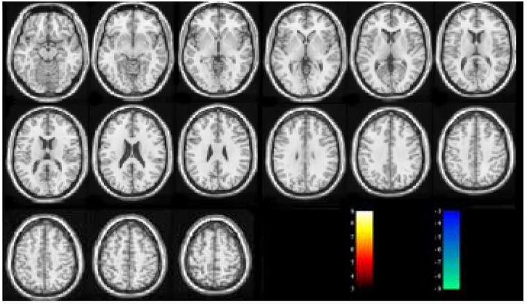
Fig. 9 shows the t maps of GLMrPM RFX (Fig. 9A) and SDMrPM RFX (Fig. 9B), superimposed on the same template as in Fig. 8. The threshold is P < 0.01 (t > 11.69, family wise error (FWE) corrected) for both group t maps, and the display window was set to 11.69 ~ 100 for easy visualization due to the large range of t values. The threshold was different from that used for assessing the results of GLM RFX and SDM RFX, because both GLMrPM RFX and SDMrPM RFX are based on the individual subject level permutations, and therefore not directly comparable to either GLM RFX or SDM RFX. With the threshold given above, SDMrPM RFX yielded very similar activation patterns to those of GLMrPM RFX, but with different peak t values, cluster extension, and average t values within the same ROIs (described in the above paragraph), as listed in Table 1.
Figure 9.

Suprathresholded t maps of A) GLMrPM RFX and B) SDMrPM RFX, using a threshold of P < 0.01(t > 11.69) (FWE corrected). The display window is 11.69 ~ 100.
SDM PMU and GLM PMU
Fig. 10 shows the suprathreshold pseudo-t (Nichols and Holmes, 2002) maps of GLM PMU and SDM PMU. Using the same threshold (P < 0.05, FWE corrected, corresponding to pseudo-t > 5.8), this figure clearly demonstrates that SDM PMU (Fig. 10B) produced larger suprathresholded clusters. Table 2 lists the result statistics of GLM PMU and SDM PMU. Consistent with Fig. 10, SDM PMU yielded higher peak pseudo-t values, larger suprathresholded clusters, and higher mean pseudo-t values. Additionally, the suprathreshold cluster of SDM PMU in visual cortex demonstrated higher significance using cluster-wise permutation than that of GLM PMU, while the cluster of SDM PMU in motor cortex presented the same cluster-wise permutation significance.
Figure 10.

Suprathresholded group level permutation pseudo-t maps of A) GLM PMU and B) SDM PMU. The threshold is P < 0.05 (FWE corrected, corresponding to pseudo-t > 5.8), and the display window is 0 ~ ±10.
Table 2.
Peak pseudo-t values, cluster extensions and within-ROI averaged pseudo-t values of SDM PMU and GLM PMU. “peak”, “ext”, “mean”, and “cluster P” represent “peak pseudo-t”, “extension of the suprathresholded cluster”, “within ROI average pseudo-t”, and “P value of the suprathresholded cluster using FWE correction”, respectively.
| Methods | Visual cortex | Motor cortex | ||||||
|---|---|---|---|---|---|---|---|---|
| peak | ext | mean | cluster P | peak | ext | mean | cluster P | |
| SDM PMU | 12.49 | 1810 | 6.7 | 0.001 | 10.15 | 538 | 5.9 | 0.001 |
| GLM PMU | 9.56 | 1126 | 5.5 | 0.001 | 8.67 | 339 | 5.1 | 0.002 |
Discussion
Two SVM-based fMRI data group analysis methods using SVM to explore the spatial activation patters of fMRI data were presented. Brain activations were represented by individual SDMs extracted by SVM classification, and population level inferences were subsequently obtained through one-sample t-testing using a “random effect model”(Penny et al., 2003), or through permutation testing (Nichols and Holmes, 2002). Extensive evaluations were performed using null hypothesis data, synthetic data, and sensory-motor fMRI data.
Using a null hypothesis ASL perfusion dataset, SDM RFX yielded almost no false detected voxels (Fig. 4) with a threshold P < 0.012, while GLM RFX presented many false detected activated or deactivated voxels (Fig. 4). Validations using synthetic functional data demonstrated that SDM RFX yielded higher detection sensitivity in terms of higher mean t value in the a priori regions than GLM RFX for every simulated signal change strength and any explored cluster size. As synthetic activations were injected to both neighboring and distant voxels and no smoothing was applied before GLM or SDM analysis, these results demonstrated that spatial activation coherence can be utilized by SVM based multivariate processing to improve the detection sensitivity. ROC analysis further demonstrated that SVM based individual level data analysis and group analysis (SDM RFX) yielded better performance (larger AUC) than GLM based individual level data analysis and group analysis (GLM RFX), respectively.
The stability of SDM extraction was verified by checking the correlation between the SDM from the whole sensory-motor fMRI dataset and the SDM from a new dataset obtained by randomly leaving out an image from the baseline condition and the task condition. The correlations were calculated for the whole brain SDM and SDM within the hypothesized activation regions. For all 10 subjects, the correlation was demonstrated to be greater than 0.975 (P < 0.00001) for the whole brain and 0.986 (P < 0.0005) for the interested regions, which proves that the SDM extraction is robust enough to represent brain discrepancy of either the whole brain or the interested regions between different conditions, and therefore validates the succeeding activation detection procedures. Applied to the sensory-motor ASL perfusion fMRI activation data, SDM RFX and SDM PMU, demonstrated increased activation detection sensitivity, compared to GLM RFX and GLM PMU, respectively, in terms of higher peak t (or pseudo-t) values, larger cluster sizes, and higher mean t (or pseudo-t) values. Although PMU may provide a more reliable comparison between SVM and GLM than RFX, since the GLM fitted model coefficient (beta) and the SDM may have different null hypothesis distributions, very consistent results were obtained by comparing SVM to GLM using RFX and PMU.
All these evaluations indicated that the SVM based data processing is more sensitive and has a lower false detection rate than the univariate data analysis. This improved performance may be attributable to the multivariate processing of spatial correlations within the functional data during SVM based classification. Since each functional image volume is treated as a unit, the spatial correlations within each volume are inherently explored by calibrating the direction of the separating vector of the optimal separating hyperplane, and thereby modulating the spatial pattern appearance of SDM. If a given spatial activation pattern consistently occurs in the functional image series, it can be more reliably detected by iteratively calibrating the main direction of the separating vector during the SVM training process than searching for this pattern independently from voxel to voxel as in the univariate approach. Additionally, compared to the GLM based approach, SVM based methods do not need an a priori modeling of the brain response, therefore they may demonstrate unexpected brain activation patterns, that might provide more comprehensive understanding of underlying neural processes of interest. Although we examined a well-characterized sensorimotor task in this report, the proposed methods are now being used to detect more subtle task or group effects in a variety of applications in our laboratory.
In the applications of the proposed method to the sensorimotor data, we used spatial smoothing as a general preprocessing step to improve the spatial SNR (Friston et al., 2000). Spatial smoothing of ASL data could yield improvements in detection of spatially extended processes without the deleterious amplification of low temporal frequency noise seen in BOLD (Wang et al., 2005a; Aguirre et al., 2005). While spatial smoothing could also increase the spatial correlations of functional data, which could potentially contribute part of the sensitivity increment, no significant improvements were demonstrated in a previous evaluations of the effect of different preprocessing parameters on SVM classifications in BOLD fMRI (LaConte et al., 2005).
Although nonlinear SVMs may provide better prediction accuracy for the brain state classification due to the feasibility of kernel tricks (Vapnik, 1995; Burges, 1998), they did not show any significant outperformance in previous applications of brain states classification (Cox and Savoy, 2003; LaConte et al., 2005). Mapping fMRI images into the hyperspace as illustrated in Fig. 1, fMRI images will be most probably aligned along certain direction (a hyperplane parallel to the first primary eigenvector of the image samples) because of each image is highly correlated to the others. Assuming subtle signal changes consistently occurred in the “on” images (images associated with functional task or contrasted brain state due to the activation related metabolism or perfusion change), their primary direction (a hyperplane parallel to the first primary eigenvector of the on images) within the hyperspace should be similar to that of the “off” (baseline) images. Given the limited number of samples, these two primary hyperplanes can be approximately treated as two parallel hyperplanes, so that a linear separating hyperplane can be always found to separate this two group of data samples with high confidence. Actually, a limited number of samples (fMRI images) in a high dimensional space (voxel space) are always linearly separable (Schölkopf and Smola, 2001) even the samples are not highly correlated. Consequently, a linear SVM should be enough to extract the brain activation discriminance as well as brain state classifications. Actually it is difficult to extract an SDM from the nonlinear SVM trained models; oppositely, linear SVM can provide several information structures to be extracted as SDMs (LaConte et al., 2005). Although we only considered the separating weight of a linear SVM model in this paper, other potential SDMs may provide more insights into the mechanism of brain functions from different point of views.
If signal changes due to brain activation are constrained to certain brain regions, a priori activation region selection could improve the classification performance since the primary hyperplanes of the “on” condition samples (within the a priori regions) and the “off” condition samples (within the same a priori regions) should be more distant from each other in the sample hyperspace than those of the whole images. A recent research has demonstrated that prior feature selection improved SVM classification for single-subject’s data (Mourão-Miranda et al., 2006). Our stability evaluations also showed that SDM could be even more stable within the prior activation regions than in the whole brain.
Treating each functional image as an independent observation without considering the acquisition time, the SVM based approaches have the disadvantage of ignoring the dynamic changes in the brain response, which can be explored using other multivariate methods such as ICA, CVA, or PLS.
The multi-subject SDM(Mourão-Miranda et al., 2005) was also validated for ASL perfusion fMRI using the sensory-motor functional data. Using the leave-one-out test, the multi-subject SDM presented a prediction precision of 75.21 percent, a little lower than that reported for BOLD fMRI data. This is probably due to the limited number of subjects scanned and the lower SNR of ASL perfusion fMRI data compared to BOLD fMRI data. According to a recent publication (Mourão-Miranda et al., 2006), the prediction performance for limited subjects can be improved by using temporal compression. Using a comparable threshold, the multi-subject SDM presented a similar activation pattern to that of GLM RFX t map.
Due to the absence of temporal noise correlation in ASL data, PMU was used to assess the significance of individual SDM or mutli-subject SDM. Using a comparable threshold, the associated multi-subject SDMrPM yielded similar activation patterns to the multi-subject SDM and the GLM RFX t map for the 10-subjects’ fingertapping ASL perfusion fMRI data. Using individual level PMU for SDM and GLM parametric maps, this paper also presented several group analysis methods for ASL perfusion fMRI by performing one-sample t-tests or group level PMU on the individual level SDMrPMs or GLMrPMs, to provide inferences on the probability of each voxel being activated or deactivated. These individual level PMU based group analyses can be used to threshold regular GLM or SDM based group analysis. For instance, we can use the suprathresholded SDMrPM RFX t map to mask the SDM RFX results. A disadvantage of both methods is that they can not provide inference on the activation clusters, since the P maps calculated in this paper are not directly connected with the activation clusters. Also, as the P map is not linearly related to the activation map (either the parametric map or SDM), due to the limited number of permutations, it is possible that every subject could have similar peak rP values in similar locations even though their activation map values are quite different. In another words, the inter-subject variability of rPM could be much less than that of the activation map. Since the t-statistics depends on the mean and the variance, both SDMrPM RFX and GLMrPM RFX could therefore yield extremely high peak t values as listed in Table 1. Instead of doing the second level statistic analysis on the rPMs, an alternative approach may be to average the individual rPMs.
Although only ASL perfusion fMRI data were tested in this paper, the proposed group analysis methods, SDM RFX and SDM PMU, are generally applicable to any fMRI data, including BOLD fMRI. To apply the individual level permutation testing based group analysis methods to BOLD fMRI, an appropriate detrending step is required to remove the low frequency signal drift (Aguirre et al., 2002). In future work, the SVM based fMRI data analyses methods will be testified in the image space not just in the eigen space, and temporal compression methods (Mourão-Miranda et al., 2006) could also be incorporated.
Acknowledgments
The authors thank Dr. Daniel Kimberg for helping setting up the Voxbo job engine; Dr. Janaina Mourão-Miranda for several communications about their previously published paper (Mourão-Miranda et al., 2005); thank Dr. John Ashburner and Dr. Yong Fan for their comments on the earliest version of this paper. This research was supported by NIH grants DA015149, RR02305, and NS045839.
Footnotes
Part of this work was presented in the 28th Annual International Conference of IEEE Engineering in Medicine and Biology Society (EMBC), 2006.
Publisher's Disclaimer: This is a PDF file of an unedited manuscript that has been accepted for publication. As a service to our customers we are providing this early version of the manuscript. The manuscript will undergo copyediting, typesetting, and review of the resulting proof before it is published in its final citable form. Please note that during the production process errors may be discovered which could affect the content, and all legal disclaimers that apply to the journal pertain.
References
- Aguirre GK, Detre JA, Wang J. Perfusion fMRI for functional neuroimaging. International Review of Neurobiology. 2005;66:213–236. doi: 10.1016/S0074-7742(05)66007-2. [DOI] [PubMed] [Google Scholar]
- Aguirre GK, Detre JA, Zarahn E, Alsop DC. Experimental design and the relative sensitivity of BOLD and perfusion fMRI. Neuroimage. 2002;15:488–500. doi: 10.1006/nimg.2001.0990. [DOI] [PubMed] [Google Scholar]
- Aguirre GK, Nichols TE, Wang JJ. Human Brain Mapping Abstracts. New York: 2003. Permutation tests for perfusion fMRI; p. 776. [Google Scholar]
- Aguirre GK, Zarahn E, D’Esposito M. The variability of human BOLD hemodynamic responses. Neuroimage. 1998;8:360–369. doi: 10.1006/nimg.1998.0369. [DOI] [PubMed] [Google Scholar]
- Allen DM. The relationship between variable selection and data augmentation and a method for prediction. Technometrics. 1974;16(1):125–127. [Google Scholar]
- Bandettini PA, Jesmanowicz A, Wong EC, Hyde JS. Processing strategies for time-course data sets in functional mri of the human brain. Magn Reson Med. 1993;30:161–173. doi: 10.1002/mrm.1910300204. [DOI] [PubMed] [Google Scholar]
- Brett M, Anton J-L, Valabregue R, Poline J-B. Region of interest analysis using an spm toolbox. 8th International Conferance on Functional Mapping of the Human Brain; 2002. Available on CD-ROM in NeuroImage. [Google Scholar]
- Brett M, Penny W, Kiebel S. Introduction to random field theory. In: Frackowiak R, Friston K, Frith C, Dolan R, Friston K, Price C, Zeki S, Ashburner J, Penny W, editors. Human Brain Function. 2 Academic Press; 2003. p. ch14. [Google Scholar]
- Bullmore ET, Rabe-Hesketh S, Morris RG, Williams SCR, Gregory L, Gray JA, Brammer MJ. Functional magnetic resonance image analysis of a large-scale neurocognitive network. NeuroImage. 1996;4:16–33. doi: 10.1006/nimg.1996.0026. [DOI] [PubMed] [Google Scholar]
- Burges CJC. A tutorial on support vector machines for pattern recognition. Data Mining and Knowledge Discovery. 1998;2:121–167. [Google Scholar]
- Buxton RB. Introduction to Functional Magnetic Resonance Imaging. Cambridge University Press; Cambridge: 2002. [Google Scholar]
- Cichocki A, Kasprzak W, Skarbek W. Adaptive learning algorithm for principal component analysis with partial data. Proc Cybernetics Syst. 1996;2:1014–1019. [Google Scholar]
- Cox DD, Savoy RL. Functional magnetic resonance imaging (fMRI) “brain reading”: detecting and classifying distributed patterns of fmri activity in human visual cortex. NeuroImage. 2003;19(2):261–270. doi: 10.1016/s1053-8119(03)00049-1. [DOI] [PubMed] [Google Scholar]
- Davatzikos C, Ruparel K, Fan Y, Shen D, Acharyya M, Loughead J, Gur R, Langleben D. Classifying spatial patterns of brain activity with machine learning methods: Application to lie detection. NeuroImage. 2005;28(3):663–668. doi: 10.1016/j.neuroimage.2005.08.009. [DOI] [PubMed] [Google Scholar]
- Detre JA, Leigh J, Williams D, Koretsky A. Perfusion imaging. Magn Reson Med. 1992;23:37–45. doi: 10.1002/mrm.1910230106. [DOI] [PubMed] [Google Scholar]
- Friston K. Brain Mapping: The Methods. Academic Press; 1996. Statistical parametric mapping and other analysis of functional imaging data; pp. 363–385. [Google Scholar]
- Friston K, Frith C, Frackowiak R, Turner R. Characterizing dynamic brain responses with fmri: A multivariate approach. NeuroImage. 1995a;2:166–172. doi: 10.1006/nimg.1995.1019. [DOI] [PubMed] [Google Scholar]
- Friston K, Frith C, Liddle F, Frackowiak R. Functional connectivity: The principal-component analysis of large (pet) data sets. Journal of Cerebral Blood Flow and Metabolism. 1993;13:5–14. doi: 10.1038/jcbfm.1993.4. [DOI] [PubMed] [Google Scholar]
- Friston K, Holmes A, Poline J, Grasby PJ, Williams SCR, Frackowiak R, Turner R. Analysis of fmri time series revisited. NeuroImage. 1995b;2:45–53. doi: 10.1006/nimg.1995.1007. [DOI] [PubMed] [Google Scholar]
- Friston K, Holmes A, Worsley K, Poline J, Frith C, Frackowiak R. Statistical parametric maps in functional imaging: A general linear approach. Human Brain Mapping. 1995c;2:189–210. [Google Scholar]
- Friston K, Jezzard P, Turner R. Analysis of functional mri time-series. Human Brain Mapping. 1994;1:153–171. [Google Scholar]
- Friston K, Josephs O, Zarahn E, Holmes A, Rouquette S, Poline J. To smooth or not to smooth? bias and efficiency in fmri time-series analysis. NeuroImage. 2000;12:196–208. doi: 10.1006/nimg.2000.0609. [DOI] [PubMed] [Google Scholar]
- Friston K, Pocock S. Repeated measures in clinical trials: An analysis using mean summary statistics and its implications for design. Statistics in medicine. 1992;11:1685C1704. doi: 10.1002/sim.4780111304. [DOI] [PubMed] [Google Scholar]
- Holmes A, Friston K. Generalisability, random effects and population inference. NeuroImage. 1998;7:S754. [Google Scholar]
- Hopfinger J, Buchel C, Holmes A, Friston K. A study of analysis parameters that influence the sensitivity of event-related fmri analyses. NeuroImage. 2000;11:326–333. doi: 10.1006/nimg.2000.0549. [DOI] [PubMed] [Google Scholar]
- Joachim T. Making large-scale svm learning practical. In: Schölkopf B, Burges C, Smola A, editors. Advances in Kernel Methods - Support Vector Learning. Cambridge Boston: MIT Press; 1999. pp. 42–56. [Google Scholar]
- LaConte S, Strother S, Cherkassky V, Anderson J, Hu X. Support vector machines for temporal classification of block design fmri data. NeuroImage. 2005;26(2):317–329. doi: 10.1016/j.neuroimage.2005.01.048. [DOI] [PubMed] [Google Scholar]
- McIntosha AR, Booksteinb FL, Haxbyc JV, Grady CL. Spatial pattern analysis of functional brain images using partial least squares. NeuroImage. 1996;3(3):143–157. doi: 10.1006/nimg.1996.0016. [DOI] [PubMed] [Google Scholar]
- McKeown MJ, Sejnowski TJ. Independent component analysis of fMRI data: Examining the assumptions. Human Brain Mapping. 1998;6(5–6):368–372. doi: 10.1002/(SICI)1097-0193(1998)6:5/6<368::AID-HBM7>3.0.CO;2-E. [DOI] [PMC free article] [PubMed] [Google Scholar]
- Metz CE. Basic principle of ROC analysis. Semin Nucl Med. 1978;VIII(4):283–98. doi: 10.1016/s0001-2998(78)80014-2. [DOI] [PubMed] [Google Scholar]
- Mitchell TM, Hutchinson R, Niculescu RS, Pereira F, Wang X, Just M, Newman S. Learning to decode cognitive states from brain images. Machine Learning. 2004;57(1–2):145–175. [Google Scholar]
- Mourão-Miranda J, Bokde AL, Born C, Hampel H, Stetter M. Classifying brain states and determining the discriminating activation patterns: Support vector machine on functional MRI data. NeuroImage. 2005;28(4):980–995. doi: 10.1016/j.neuroimage.2005.06.070. [DOI] [PubMed] [Google Scholar]
- Mourão-Miranda J, Reynaud E, McGlone F, Calvert G, Brammer M. The impact of temporal compression and space selection on SVM analysis of single-subject and multi-subject fMRI data. NeuroImage. 2006;33:1055–1065. doi: 10.1016/j.neuroimage.2006.08.016. [DOI] [PubMed] [Google Scholar]
- Nichols T, Holmes A. Nonparametric permutation tests for functional neuroimaging: A primer with examples. Human Brain Mapping. 2002;15:1–25. doi: 10.1002/hbm.1058. [DOI] [PMC free article] [PubMed] [Google Scholar]
- Penny W, Holmes A, Friston K. Random effects analysis. In: Frackowiak R, Friston K, Frith C, Dolan R, Friston K, Price C, Zeki S, Ashburner J, Penny W, editors. Human Brain Function. 2 Academic Press; 2003. p. ch12. [Google Scholar]
- Press W, Teukolsky S, Vetterling W, Flannery B. Numerical Recipes in C++: the art of scientific computing. 2 Cambridge University Press; 2002. [Google Scholar]
- Schölkopf B, Smola A. Learning with Kernels: Support Vector Machines, Regularization, Optimization, and Beyond. MIT Press; 2001. [Google Scholar]
- Vapnik V. The Nature of Statistical Learning Theory. Springer-Verlag; New York: 1995. [Google Scholar]
- Vetterling WT, Flannery BP. Numerical Recipes in C++: The Art of Scientific Computing. 2 Cambridge University Press; New York: 2002. [Google Scholar]
- Wang JJ, Wang Z, Aguirre GK, Detre JA. To smooth or not to smooth?- ROC analysis of perfusion fMRI data. Magnetic Resonance Imaging. 2005a;23:75–81. doi: 10.1016/j.mri.2004.11.009. [DOI] [PubMed] [Google Scholar]
- Wang JJ, Zhang Y, Wolf RL, Roc AC, Alsop DC, Detre JA. Amplitude modulated continuous arterial spin labeling perfusion mr with single coil at 3t:feasibility study. Radiology. 2005b;235(1):218–28. doi: 10.1148/radiol.2351031663. [DOI] [PubMed] [Google Scholar]
- Wang X, Hutchinson R, Mitchell T. Training fMRI classifiers to discriminate cognitive states across multiple subjects. Proc. of 17th Annual Conference on Neural Information Processing Systems; Vancouver and Whistler, Canada. 2003a. [Google Scholar]
- Wang Z, Lee Y, Fiori S, Leung C, Zhu Y. An improved sequential method for principal component analysis. Pattern Recognition Letters. 2003b;24(9–10):1409–1415. [Google Scholar]
- Wang Z, Wang J, Calhoun V, Rao H, Detre JA, Childress AR. Strategies for reducing large fmri data sets for independent component analysisfunctional connectivity in the resting brain: A network analysis of the default mode hypothesis. Magnetic resonance imaging. 2006;24(5):591–596. doi: 10.1016/j.mri.2005.12.013. [DOI] [PubMed] [Google Scholar]
- Wang Z, Wang J, Childress AR, Rao H, Detre JA. Crls-pca based independent component analysis for fMRI study. Proceedings EMBC-05. 2005c:5904–5907. doi: 10.1109/IEMBS.2005.1615834. [DOI] [PubMed] [Google Scholar]
- Wong E. Potential and pitfalls of arterial spin labeling based perfusion imaging techniques for MRI. In: Moonen CW, Bandettini P, editors. Functional MRI, Medical Radiology:Diagnostic Imaging and Radiation Oncology. New York: Springer-Verlag; 1999. pp. 63–69. [Google Scholar]
- Worsley K, Friston K. Analysis of fmri time-series revisited - again. NeuroImage. 1995;2:173–181. doi: 10.1006/nimg.1995.1023. [DOI] [PubMed] [Google Scholar]
- Worsley KJ, Poline JB, Friston KJ, Evans AC. Characterizing the response of PET and fMRI data using multivariate linear models. NeuroImage. 1997;6:305–319. doi: 10.1006/nimg.1997.0294. [DOI] [PubMed] [Google Scholar]