Receptive fields and functional architecture in the retina

Abstract

Functional architecture of the striate cortex is known mostly at the tissue level – how neurons of different function distribute across its depth and surface on a scale of millimetres. But explanations for its design – why it is just so – need to be addressed at the synaptic level, a much finer scale where the basic description is still lacking. Functional architecture of the retina is known from the scale of millimetres down to nanometres, so we have sought explanations for various aspects of its design. Here we review several aspects of the retina's functional architecture and find that all seem governed by a single principle: represent the most information for the least cost in space and energy. Specifically: (i) why are OFF ganglion cells more numerous than ON cells? Because natural scenes contain more negative than positive contrasts, and the retina matches its neural resources to represent them equally well; (ii) why do ganglion cells of a given type overlap their dendrites to achieve 3-fold coverage? Because this maximizes total information represented by the array – balancing signal-to-noise improvement against increased redundancy; (iii) why do ganglion cells form multiple arrays? Because this allows most information to be sent at lower rates, decreasing the space and energy costs for sending a given amount of information. This broad principle, operating at higher levels, probably contributes to the brain's immense computational efficiency.

David Hubel often remarked (paraphrasing Lord Rutherford) that, if an experiment required statistics, it was probably not worth doing. As a student, I (P.S.) took this to mean that we should be looking for large effects and not wasting effort to tease out small ones from noise. Of course, that was easy to say once he and Torsten Wiesel had discovered their huge effects, such as sensitivity of cortical neurons to stimulus orientation and direction, binocular receptive fields, orientation and ocular dominance columns, and the drama of monocular deprivation – effects so robust that we are now celebrating their 50th anniversary!

Unfortunately, through no fault of David's, I also took the comment to mean that the brain works deterministically, not statistically. This notion is easily entertained while exploring receptive fields with high contrast stimuli. When you find just the right ‘trigger feature’, the neuron fires sharply and reliably – so why fuss about statistics or the brain's supposed stochastic nature? Nor were we to concern ourselves with what David and Torsten term ‘theory, sometimes called computation’, which they still regard as ‘an example of illnesses that scientific fields can be subject to’ (Hubel & Wiesel, 2004). Of course, while we were preoccupied for decades simply describing compelling effects and architectures, any effort to use theory to explain them, that is, to investigate why they are organized just so, seemed misguided. But it was not misguided; it was merely premature, and it was on the wrong scale.

Functional architecture must eventually be studied on the scale of synaptic circuits

Knowledge regarding functional architecture of striate cortex has accumulated mostly at the tissue level – how neurons of different function distribute across its depth and surface – a scale of millimetres (Hubel & Wiesel, 2004). But explanations regarding the underlying design must be addressed at the synaptic level – a finer scale where connectivity is still unknown. For example, there is no consensus regarding how many types of cell are present, nor how to define a cortical cell type, nor even whether ‘types’ really exist! Nor is it known how the primary thalamic afferents connect to different cells, let alone how these cells connect locally with each other (e.g. Callaway, 2005; Douglas & Martin, 2007; Xu & Callaway, 2009). There are good reasons for this continuing state of ignorance.

One is technical: to identify a synapse requires 10 nm resolution (the width of the synaptic cleft) whereas conventional light microscopy resolves at best 200 nm. Therefore, to identify a ‘circuit’ by light microscopy requires inference to bridge this order of magnitude deficit in resolution, and this led the boldest, most inspired neuroanatomist, Ramón y Cajal, into serious errors. Another challenge is posed by the devilish arrangements along the vertical axis. One might have hoped that the layering of cortical neurons would help in working out their circuits. But within a layer, neurons are as diverse as tree species in a tropical rainforest – and each type connects differently across layers. This arrangement is probably fundamental to cortical architecture – but it renders pointless trying to understand a circuit by taking the average connection and looking for broad patterns. Working out the connections of one neuron, you will need to travel tangentially for hundreds of micrometres to find another exactly like it.

Electron microscopy offers the essential resolution, easily identifying a synapse such as a thalamic bouton contacting a dendritic spine. But it cannot identify either the afferent that produced the bouton, nor the dendrite that produced the spine. The processes become too fine (<100 nm) to trace through conventional serial sections; and even if one could, the distances are orders of magnitude too great. New technologies are changing all this, but for now if you want to consider neural architecture in sufficiently fine detail to explain a design, you must turn to the retina – where both function and architecture at the circuit level have been quantified. And there one soon discovers that the explanations require both of David Hubel's bêtes noir: statistics and theory.

Understanding circuits requires statistical reasoning and ‘theory’

Vision is limited by statistical fluctuations whose sources are now fairly well identified. For example, when a short row of retinal ganglion cells is excited, we perceive an edge. But if the edge has low contrast (∼1%) and appears only briefly (∼100 ms), whether we see it or not is a matter of chance. In bright light, the chance is decent, near 70%, but in dim light, we are reduced to guessing. Light intensity matters for a purely statistical reason: photons (light quanta) arrive stochastically. Obeying Poisson statistics, their signal-to-noise ratio (SNR) equals the mean number of photons (n) divided by n. This explains why detection, say for birding or hunting, is improved by expensive optics – they collect photons more efficiently.

One can compute (using a model that includes the eye's optics and the efficiency of photon capture) how much information should be available from a given stimulus for detection by neural circuits. Compared to this calculation, actual detection measured psychophysically is less sensitive by about 10-fold, and this factor is constant across light intensities. This difference represents a loss of information due to neural noise within the retina (Borghuis et al. 2009). Here, too, the cause is statistical fluctuation – of transmitter quanta at each of the retina's two synaptic stages. Because transmitter quanta also follow the Poisson statistics, the neural signal-to-noise ratio improves as n. It seems shocking that neural noise should degrade visual sensitivity by a full log unit. Why would natural selection produce such shoddy circuits when we might potentially see 10-fold better – and possibly be 10-fold smarter? This question certainly warrants scrutiny of the circuit designs.

It emerges that retinal circuits are not ‘optimal’. They could be bolstered in various ways to relay more information and thus improve vision. For example, SNR could be improved by adding more synapses and/or by raising release rates. But synapses occupy space; and transmitter quanta discharge ionic batteries, whose recharging requires energy (Attwell & Laughlin, 2001). Moreover, increased investment brings diminishing returns; for example, doubling SNR requires quadrupling transmitter quanta.

Here, using four examples from mammalian retina (guinea pig), we explore the broad hypothesis that neural circuits are designed to send a given quantity of information using the least resources. Following sensible rules and making compromises, the retina: (i) allots resources according to the probable return of information; (ii) structures neuronal arrays to maximize information by balancing increased SNR against increased redundancy; (iii) uses multiple parallel circuits to send more information at lower rates, and thus at lower cost in space and energy.

Each of our examples requires calculations based on Shannon's equations – that is, on ‘information theory’. ‘Information’ in Shannon's sense is a signal statistic that broadly limits the quality of decisions that are based on observations of the signal. For a channel with Gaussian signals and additive Gaussian noise, Shannon's formula for information is intuitive:

(1)

where SNR, the signal-to-noise-ratio, is the signal variance divided by the noise variance. This formula amounts to a summary statistic that distills communication power from three key aspects of a signal – its bandwidth (here parameterized by signal variance), how well the bandwidth is used (here with a Gaussian distribution), and the noise (here parameterized by noise variance). Since natural visual stimuli are not Gaussian we will sometimes need a more general formula. Given a probability distribution for the joint responses of N signalling elements, the total amount of information that could be carried by the signals is given by a quantity called the ‘entropy’ of the signal:

(2)

In our analyses, the loss of information to noise is approximately incorporated in this formula by discretizing the c_i into distinguishable signalling levels that reflect the noise.

Since the retinal output provides the basis for all visual behaviour, and not just a single well-specified task, a broad statistic of this kind is necessary to evaluate retinal performance. A precise formulation of our hypothesis is that, given the information required for behaviour, the retina minimizes its computational costs. In practice, it is often easier to specify the cost in terms of amount of resources expended by a circuit and to ask how it should then be organized to maximize information. The goal of such a theory is 2-fold – to explain the underlying rationale for known structural and functional organization, and to predict new effects that would guide the design of experiments. Eventually such a strategy applied to the whole brain might help explain how our brain can deliver such amazing computing power in a volume no greater than a laptop and drawing no more power than a refrigerator light bulb.

Some ‘whys’ in retinal design

Resource allocation by ON and OFF ganglion cell arrays

The cone's representation of light intensity is converted at the first retinal synapse to a representation of local contrast and then routed to two classes of second order (bipolar) cell. One class depolarizes to positive contrasts (ON), and the other depolarizes to negative contrasts (OFF) (Fig. 1A). Surprisingly, more resources are devoted to circuits for negative contrasts: OFF bipolar cells outnumber ON bipolar cells by 2-fold (Ahmad et al. 2003). This asymmetry carries forward to the ganglion cells: OFF cells have narrower dendritic fields (Fig. 1B and C) and 1.3-fold more overlap (Borghuis et al. 2008), implying an OFF/ON ratio of ∼1.7. Similar differences are found across species (rat: Morigiwa et al. 1989; rabbit: DeVries & Baylor, 1997; monkey: Chichilnisky & Kalmar, 2002; human: Dacey & Petersen, 1992) and across cell types, (e.g. ‘midget’ and ‘parasol’ in human; Dacey & Petersen, 1992). These differences persist at least as far as striate cortex.

Figure 1. Dendritic arbors of OFF ganglion cells are smaller but more densely branched.

A, retina in radial view. The first synapse routes the photosignal to two classes of bipolar neuron, one excited by negative contrasts (OFF cells) and another class excited by positive contrasts (ON cells). These signals are rectified by voltage-sensitive calcium channels at the bipolar cell synapses to OFF and ON ganglion cells. The ON arbor is broad and sparsely branched whereas the OFF arbor is narrower and more densely branched. B, ON and OFF ganglion cells (brisk-transient class) in flat view. Cells were injected with fluorescent dye and photographed in the confocal microscope. The ON arbor is broad and sparsely branched whereas the OFF arbor is narrower and more densely branched. C and D, dendritic field area is smaller for OFF than for ON cells, but total dendritic lengths are the same and collect similar numbers of bipolar synapses (Xu et al. 2008) (adapted from C. Ratliff, Y.-H. Kao, P. Sterling & V. Balasubramanian, unpublished observations). IPL, inner plexiform layer.

Another key difference is that OFF dendritic arbors branch more densely (Fig. 1B; Morigiwa et al. 1989; Kier et al. 1995; Xu et al. 2005; C. Ratliff, Y.-H. Kao, P. Sterling & V. Balasubramanian, unpublished observations). Consequently, despite its narrower dendritic field, an OFF cell has the same total dendritic length as the corresponding ON cell (Fig. 1D; C. Ratliff, Y.-H. Kao, P. Sterling & V. Balasubramanian, unpublished observations); thus they receive similar numbers of synapses (Xu et al. 2008). Given the excess of OFF cells, this implies that the OFF array employs ∼1.7-fold more excitatory synapses. In short, the OFF array, being denser than the ON array, allocates more total resources to represent a scene. An individual OFF cell uses roughly the same resources as an ON cell but concentrates on a smaller region of the scene (C. Ratliff, Y.-H. Kao, P. Sterling & V. Balasubramanian, unpublished observations). This leads to a theoretical question: why should the retina (and later stages of the visual system) devote more resources to OFF cells?

Our broad hypothesis predicts that the excess resources devoted to OFF circuits should be matched to an excess of information present in negative contrast regions of natural scenes. This suggests, surprisingly, that natural images contain more dark spots (negative contrasts) than bright spots (positive contrasts). This was tested quantitatively by employing a standard model of a centre-surround receptive field (C. Ratliff, Y.-H. Kao, P. Sterling & V. Balasubramanian, unpublished observations). This is a difference-of-Gaussians filter (Rodieck, 1965), divisively normalized (Tadmor & Tolhurst, 2000). This filter measured local spatial contrast at an image point (x,y) as

(3)

Here I_c and I_s are the intensities measured by normalized centre and surround Gaussian filters centred at (x,y). The relative extents of the centre and surround were taken to lie in the physiologically measured range (e.g. Linsenmeier et al. 1982); the divisive normalization captured the ganglion cell's adaptation to local mean luminance (Troy & Robson, 1992; Brady & Field, 2000). Thus, the filter measured contrast as the per cent difference in intensity between centre and surround: a positive response meant that the centre was brighter than surround, and a negative response meant that the centre was darker than the surround.

Images were selected from a standard set (van Hateren & van der Schaaf, 1998) and convolved with the filter to measure contrast at every location (Fig. 2A, B and C; C. Ratliff, Y.-H. Kao, P. Sterling & V. Balasubramanian, unpublished observations). For all filter sizes, the distributions of local contrast peaked sharply at zero, and negative contrasts were about 50% more numerous. The excess of negative contrasts was robust to changes in receptive field shape and divisive normalization, thus matching the prediction from retinal architecture (Ratliff et al. 2009). The dark–bright asymmetry arises from the skewed intensity distribution in natural scenes (low peak, long tail, approximately log-normal form; Richards, 1982) and persists across scales because of the presence of long-range spatial correlations (Field, 1987; Ruderman & Bialek, 1994; Simoncelli & Olshausen, 2001). Having found a clear asymmetry for natural images in their numbers of dark and bright regions, and the statistical origin of this effect, we asked what mosaic of ganglion cells selective for dark and bright contrasts would maximize the information transmitted from natural images.

Figure 2. Natural images contain more negative than positive contrasts at all scales. Correspondingly the optimal mosaic contains more OFF cells.

A, centres of difference-of-Gaussians filters superimposed on an image. B, contrast distributions at three scales: the distributions are skewed, and negative contrasts are more abundant. C, proportion of negative, positive and subthreshold (<3%) contrasts. At all scales negative contrasts are ∼50% more numerous. The proportion of subthreshold contrasts declines with scale because distributions in B flatten with increasing centre radius. D, in the optimal mosaic OFF filters are more numerous and smaller than the ON filters. Here 16 filters cover 25 image pixels, and information in bits is maximized when 12 of the filters are of the OFF type (adapted from C. Ratliff, Y.-H. Kao, P. Sterling & V. Balasubramanian, unpublished observations).

Optimal mosaics use more OFF cells

Given the excess of negative contrasts, it is natural to hypothesize that the optimal mosaic should have more OFF cells. To see this, suppose first that the retina contains only one ganglion cell. Should the cell be OFF or ON? Evidently, it should be an OFF cell because it is more likely to respond to a natural image and hence will be more informative. This excess should persist for denser arrays. To further analyse this idea we made a model of difference-of-Gaussian filters, followed by a rectifying non-linearity that transformed negative or positive filter responses into 10 discrete, equally probable firing levels (Laughlin, 1981; Dhingra & Smith, 2004). The discretization and number of firing levels reflected measurements of thresholding behaviour and noise in ON and OFF ganglion cell responses (Dhingra et al. 2003; Xu et al. 2005).

The information captured from an image by such an array is equal to its response entropy (Shannon & Weaver, 1949; Ruderman & Bialek, 1994). Entropy is computed from the joint distribution of responses of the array (eqn (2)). This was measured by scanning rectangular arrays of ON or OFF filters across each image to enumerate contrast responses. It was then asked: what array geometries maximize information represented from natural images (C. Ratliff, Y.-H. Kao, P. Sterling & V. Balasubramanian, unpublished observations)? To study this, N=N_OFF+N_ON model receptive fields were restricted to cover a region of fixed area with rectangular OFF and ON arrays. The assumption of rectangular arrays set cell spacing. For each partition of N into N_OFF+N_ON, we independently varied ON and OFF receptive field sizes to maximize information from each array. Figure 2D shows an example where 16 receptive fields, covering 25 pixels, conveyed the most information when OFF receptive fields were about twice as numerous as ON and ∼20% narrower. For all choices of filter density (1–100 pixels per filter) and number (10–100 filters), as well as a wide range of receptive field shapes and normalizations, the optimal mosaic always contained a denser OFF array (C. Ratliff, Y.-H. Kao, P. Sterling & V. Balasubramanian, unpublished observations).

In summary, the question, ‘why does the retina express an excess of OFF cells?’ seems to be answered. This arrangement would produce the greatest gain of information for the least overall cost. The result apparently generalizes across cell types and species, although specific comparisons require additional information, e.g. noise, specific receptive field shapes, variations in environmental image statistics, and differences in behaviour. But meanwhile, a statistical analysis of natural images coupled with a theoretical analysis of optimal information transmission appears to explain an otherwise surprising asymmetry. We also found that each individual OFF element in the optimal mosaic transmits as much information as a larger ON element. This correlates with (and probably explains) the anatomical finding that smaller OFF cells express similar numbers of synapses as larger ON cells (Fig. 1D; Kier et al. 1995; Xu et al. 2008), suggesting another principle to connect neural anatomy and information transfer: equal numbers of synapses for equal bits (Sterling, 2004).

Overlap of dendritic fields and receptive field centres

Ganglion cell mosaics have been described as ‘tiling’ the retina. Actually, however, neighbouring cells of the same type substantially overlap their dendrites to produce nearly 3-fold coverage (Wässle, 2004). Moreover, because receptive field centres are somewhat broader than the corresponding dendritic fields, their coverage is even greater. For example, the coverage factor (field area × cell density) for centres of the ON brisk-transient cell is ∼4, and for the OFF brisk-transient cell, it is ∼6 (Fig. 3A and B; Borghuis et al. 2008), and this is true for many other cell types (DeVries & Baylor, 1997). As synapses distribute on the membrane at a constant density (Freed et al. 1992; Kier et al. 1995; Calkins & Sterling, 2007; Xu et al. 2008, such extensive dendritic overlap uses many more synapses than would be required for simple tiling. This leads to another theoretical question: why should the retina devote additional resources to such expensive overlap?

Figure 3. Neighbouring ganglion cells overlap their dendritic fields and receptive field centres.

A, dendritic fields of an OFF/OFF pair typically overlap by about 40%. B, OFF/OFF and ON/ON neighbours share similar temporal and spatial filters. Left: temporal filters superimpose (spike-triggered average of responses to white noise). Right: spatial response profiles, fitted with difference-of-Gaussians functions, show that neighbouring ganglion cell receptive fields overlap substantially. Here receptive field centres are spaced at 2.1 σ of the centre Gaussian for (ON/ON) and 1.7 σ for (OFF/OFF), corresponding, respectively, to receptive field coverage factors of 4.1 and 6.1. C, spatial resolution of the array is set by cell density. Narrow receptive fields have low overlap and low mutual redundancy, but also receive fewer synapses and thus have low signal-to-noise ratio (SNR). Wide receptive fields have high overlap and high mutual redundancy, but also receive more synapses and thus have high SNR (adapted from Borghuis et al. 2008).

Cell spacing in an array sets the visual acuity required for behaviour (Wässle & Boycott, 1991). Therefore, we took cell spacing as given and expressed the degree of receptive field overlap in terms of the standard deviation (σ) of the Gaussian centre (Borghuis et al. 2008). This transformed the question to: why do most ganglion cell arrays use 2 σ spacing?

To explain receptive field overlap we recall that detection performance based on the retinal output is set for many tasks by the amount of represented information (Geisler, 1989; Cover & Thomas, 1991; Thomson & Kristan, 2005). A larger receptive field collects more information – because there is input from more cones, and this input is conveyed by more synapses. This increases SNR, and information increases as log₂ of the SNR (eqn (1)). On the other hand, for fixed cell spacing, larger receptive fields overlap more (Fig. 3C); thus, some of the information carried by neighbours is redundant. As a cell's response range is finite, the redundancy due to overlap tends to reduce the array's total information. Thus, we hypothesized that receptive field overlap should balance the advantage of greater SNR against the disadvantage of greater redundancy.

To estimate this trade-off, we approximated a ganglion cell response as a Gaussian information channel and related the information represented by an array of such cells to the SNR of cones and the array overlap by the formula

(4)

Here N is the number of cells in the array; f² measures the SNR improvement of a receptive field due to summation over cones (computed following Tsukamoto et al. 1990); and ρ discounts for the redundancy in the responses of overlapping array elements (computed following C. Ratliff, Y.-H. Kao, P. Sterling & V. Balasubramanian, unpublished observations). ON and OFF arrays were modelled with fixed spacing and difference-of-Gaussian receptive fields with shapes (centre/surround ratio, surround strength) that had been measured experimentally (Borghuis et al. 2008). Then the redundancy discount ρ, the SNR improvement f², and the total information in the array I_array were functions only of the size of the receptive fields, measured here in terms of the centre standard deviation σ, while receptive field overlap was quantified as receptive field spacing measured in units of σ. Larger spacing in units of σ indicates less receptive field overlap. The hypothesis was that receptive field overlap would be set to maximize the array's total information (I_array).

Optimal overlap in a ganglion cell array

Natural scenes have a distinct statistical structure: spatial correlations decay as 1/spatial frequency (Field, 1987); furthermore, the distribution of intensities is skewed (Richards, 1982). Taking natural scenes as input to our model ganglion cell array (Fig. 4A; van Hateren & van der Schaaf, 1998), information represented in the model array peaked when the spacing was 1.9 σ (ON) and 1.8 σ (OFF) (Fig. 4B). Thus, optimal overlap was slightly greater for the OFF array. Furthermore, the range of measured receptive field spacings (ON: 2.05 ± 0.50 σ; OFF: 1.86 ± 0.55 σ) tightly bracketed the computed optimum. Importantly, the optimum lay far from the ∼4 σ spacing required for simple ‘tiling’ without overlap.

Figure 4. Information about natural scenes is maximized when receptive fields are spaced at about twice the standard deviation of the centre Gaussian.

A, information was measured for a receptive field array stimulated with natural images. Left inset: array superimposed on small patch of natural image. Right inset: array superimposed on small patch of white noise. B, information from natural images peaks at a receptive field (RF) spacing of ∼2 σ. Bars show the range of measured receptive field separations for ON (open) and OFF (filled). Tested with synthetic ‘natural’ images (see main text), information peaks at the same receptive field spacing as for natural scenes. Information represented from white noise images increases monotonically, but gradually, with centre spacing in units of σ. Hence the optimal array for white noise has large spacing and minimal receptive field overlap. C, optimal spacing is robust to differences in width of receptive field surround: a 2-fold expansion leaves optimal spacing within the measured range (ON: open bar; OFF: filled bar). Surround widths much larger (≫ 2-fold) than the measured width lead to widely spaced optimal arrays (>3 s) with bumpy contrast sensitivity surfaces. D, optimal spacing is robust to changes in estimated cone SNR: over four orders of SNR optimal array spacing remains within the measured range (adapted from Borghuis et al. 2008).

The putative advantage of overlap is to allow cells to expand their centres and so improve SNR by averaging spatially correlated signals. If so, overlap would confer no advantage for images that lack spatial correlations. This was tested by studying the optimal array for representing spatial white noise, which by definition lacks correlations (Fig. 4A, right inset; Borghuis et al. 2008). The separation of centres was fixed while centre width (hence overlap) was varied. As overlap decreased (and spacing expressed as σ increased), the total represented information gradually increased (Fig. 4B). Thus, the optimal spacing minimizes receptive field overlap. However, because the rate of increase is slow, there is little advantage to selecting a particular array spacing provided it is greater than ∼2 σ. This suggests that the strongly conserved 2 σ spacing of ganglion cell arrays is a specific adaptation to the statistical regularities of natural images.

To test what properties of natural scenes set the optimal spacing, we asked what array would be optimal for representing ‘natural pink noise’, synthetic images that mimic the statistical properties of natural scenes: the 1/f power spectrum (Field 1987) and the skewed intensity distribution (Richards, 1982). For these synthetic images, the amount of information represented by the array is greater than for natural scenes, because natural pink noise, lacking higher order correlations, is less redundant. Nevertheless, the optimal array spacing for the synthetic images is identical to that for natural scenes (1.9 σ for model ON receptive fields, Fig. 4B). This demonstrates that the skewed intensity distribution and 1/f power spectrum of natural images is sufficient to explain the optimal array spacing (Borghuis et al. 2008).

These results were robust to changes in the model – with a surround/centre ratio that was 2-fold wider than measured, the optimum remained within the range of spacings measured in the retina. Moreover, across the range of tested surround widths (1.25–5 σ), the optimal array always showed substantial receptive field overlap and never showed simple tiling (Fig. 4C). Likewise, the optimal array overlap was essentially constant across five orders of magnitude of variation in the assumed cone SNR (Fig. 4D).

In summary, the question, ‘why do ganglion cells of a given type extensively overlap their fields?’ seems to be answered. Overlap, such that every point in space is covered by ∼3 dendritic fields, causes the Gaussian receptive field centres to be spaced at ∼2 standard deviations (σ). For natural images, this balances increased SNR against increased redundancy and thus maximizes information represented by the array. This effect arises from the statistical properties of natural scenes, for it is absent when tested on images lacking spatial correlations (white noise) and fully present when tested on artificial images containing the key properties (natural pink noise). Thus, overlap in a ganglion cell array co-operates with single-cell synaptic weighting to improve vision by optimally representing the statistical structure of natural scenes.

Information capacity of different ganglion cell types

The retina expresses ∼10–15 distinct types of ganglion cell (Masland, 2001; Wässle, 2004). Each type responds to distinct aspects of a scene and conveys this information via characteristic firing patterns (Fig. 5; Koch et al. 2006). For example, the brisk-transient (Y) cell fires to a broad range of temporal and spatial frequencies with brief, sharply timed bursts whereas the brisk-sustained (X) cell fires similarly but is tuned to higher spatial and lower temporal frequencies. ‘Sluggish’ cells tend to fire at lower rates with less temporal precision and to be more selective for particular features, such as a local edge or direction of motion.

Figure 5. Firing patterns to different types of natural motion are similar within a cell type but different across types.

Here five cells were recorded simultaneously on a multi-electrode array. Each cell responded similarly to all three motion stimuli. The brisk-transient and ON–OFF direction-selective (DS) cells responded with high peak rates and low firing fractions whereas the brisk-sustained, ON DS, and local-edge cells responded with lower peak rates and higher firing fractions. The brisk-transient and ON–OFF DS responses showed the lowest spike-time jitter across trials whereas the brisk-sustained and local-edge responses showed the highest. For sluggish types, mean firing rates were about half that of the brisk cell types (adapted from Koch et al. 2006).

These characteristic response patterns are conserved across a broad range of naturalistic stimuli. This is visually apparent in Fig. 5 and has been confirmed statistically (Koch et al. 2006). Despite the clear differences in firing patterns across cell types, the mean rates evoked by naturalistic stimuli are remarkably similar. Although the peak firing rates to ‘tuned’ stimuli can vary 100-fold between the brisk and sluggish classes, the mean rates to naturalistic movies vary by only about 2-fold: ∼6 Hz (local-edge) vs∼13 Hz (brisk-transient). Thus, although different types can achieve vastly different levels of activity, under natural conditions they are tuned to fire at similar mean rates (∼10 Hz).

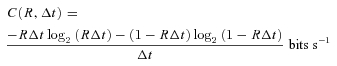
How much information does each cell type encode in response to naturalistic stimuli? Cells with higher spike rates have greater intrinsic information capacity simply because they fire more; but some cells might make better use of their capacity, i.e. might show greater coding efficiency. Coding capacity is the maximum total information rate possible, given the mean spike rate (Rieke et al. 1999; Koch et al. 2004). It is achieved when spikes are independent (no temporal correlations) and when the spike train is perfectly reproducible (no noise entropy). Coding capacity, C, is calculated as:

(5)

where R is mean spike rate and Δt= 5 ms, i.e. the time bin used to calculate information. Coding efficiency is a cell's actual information rate divided by its coding capacity.

Coding capacity differs across types – with means ranging from ∼20 bits s⁻¹ for direction-selective and local-edge cells to ∼40 bits s⁻¹ for brisk cells – simply because of the differences in mean firing rates (Koch et al. 2006) However, coding efficiency is identical across types and across stimuli: ∼26% of capacity (Fig. 6A). Consequently, the average information per spike (information rate/mean spike rate) was highest for the lowest spike rate: ∼3.5 bits spike⁻¹vs∼1 bit spike⁻¹ for the highest rate (Fig. 6B). This accords with the principle of information theory that rarer events carry more information per event (Shannon & Weaver, 1949; Zador, 1998). Accordingly, cells with lower mean spike rates (typically ON direction-selective, ON–OFF direction-selective, and local-edge) sent ∼20% more bits spike⁻¹ than the brisk types.

Figure 6. All cell types transmit information with similar efficiency.

Information rate (total entropy – noise entropy) was estimated by the direct method (Koch et al. 2006). A, continuous line shows the coding capacity (C(R)) of a ganglion cell at a given firing rate. This is the information rate assuming a Poisson process with each interval independent). Coloured dots show information rates for each recorded cell, and for all types of stimuli. Dashed line shows the best fit to information rate as a fraction of coding capacity: I(R) = 0.26 C(R). Information rate for all cell types and stimuli was thus ∼26% of coding capacity. B, dashed line indicates the information per spike 0.26 * C(R)/R. Lower rates carry more bits per spike. B-T, brisk-transient; B-S, brisk-sustained.; LE, local-edge. (Adapted from Koch et al. 2006.)

From these measurements we constructed an ‘information budget’ for the guinea pig optic nerve. The measured information rate for each type times the number of cells of that type suggest that the nerve's ∼100 000 axons send ∼875 000 bits s⁻¹. Extrapolating to the human retina with ∼10⁶ ganglion cells gives an estimated information rate comparable to an Ethernet cable (Koch et al. 2006). This information distributes asymmetrically across the different ganglion cells channels (Fig. 7). The sluggish types contribute 64% of the information, far outscoring the brisk types. Indeed, since most studies of ganglion cell coding have focused on the brisk types (X and Y in cat; M and P in primate), it is startling to realize that the famous Y cells contribute only 9% of the information sent down the optic nerve; whereas the more mysterious local-edge cells contribute nearly twice as much!

Figure 7. How information traffic is parcelled among cell types.

Most information is sent over the optic nerve, not by the most familiar ‘brisk’ cells (X and Y) but rather by a diverse population of ‘sluggish’ cells.

Why does the retina need so many cell types?

Given this coding strategy, i.e. roughly similar information rates and equal coding efficiency across cell types, why does the retina not send all its information at a high rate over one cell type? Probably because the energetic cost of signalling by an axon increases non-linearly with temporal frequency and information rate (Levy & Baxter, 1996; Laughlin et al. 1998; Balasubramanian et al. 2001). To illustrate, compare the cost of transmitting 300 bits s⁻¹ over a bundle of independent axons with mean spike rates of 4 Hz (local-edge), 8 Hz (brisk-transient) and 40 Hz (hypothetical high-rate channel) (Table 1). Given 26% efficiency, the 4 Hz neuron sends 2.1 bits spike⁻¹, the 8 Hz neuron sends 1.8 bits spike⁻¹ and the 40 Hz neuron sends only 1.1 bits spike⁻¹ (from Fig. 6A). Thus, for 300 bits s⁻¹ the ‘local-edge’ cable would use ∼140 spikes s⁻¹, the ‘brisk-transient’ cable ∼170 spikes s⁻¹ and the high-rate cable ∼270 spikes s⁻¹. Since the dominant metabolic cost in neural signalling is associated with spiking (Attwell & Laughlin, 2001; Lennie, 2003), the cables with lower firing rates would save considerable energy. Likewise, theoretical studies predict that metabolic cost is minimized when signals are distributed over many weakly active cells (Sarpeshkar, 1998).

Table 1.

Transmitting information at low mean rates saves spikes

Comparison of three kinds of neural cables
Type	Local edge	Brisk-transient	Super
Mean spike rate for cell	4 Hz	8 Hz	40 Hz
Bits spike−1	2.1	1.8	1.1
Spikes s−1 for 300 bits s−1 traffic over cable	∼140	∼170	∼270

Cables where each fibre transmits information at 4 Hz (the lowest rate for ganglion cells) and at 8 Hz (median rate for ganglion cells) require similar numbers of spikes to transmit 300 bits s⁻¹. A hypothetical cable with 40 Hz fibres requires substantially more spikes for the same information rate (adapted from Koch et al. 2006).

Of course, there are other reasons to use multiple cell types (Sterling, 2004). Spatial acuity requires narrow-field cells with a high sampling density (Wässle & Boycott, 1991). The high density demands that each cell's information rate should be low to reduce costs. On the other hand, encoding high stimulus velocity requires extended spatial summation and thus a broad-field cell – plus the ability to transmit at high bit rates so as not to lose the higher temporal frequencies. Such a type must necessarily be expensive, but given the extended dendritic field, this type can be sparse. Consequently, energetic considerations probably interact with other constraints to set the number of types and a general information rate of roughly 10 bits s⁻¹ and ∼2 bits spike⁻¹.

Functional architecture of the optic nerve

The retina's information budget shows a marked asymmetry: most information is conveyed by a diverse population of small, low-rate cells (Fig. 7). We wondered if this asymmetry might have a structural correlate in the optic nerve. Electron micrographs of the nerve show axon profiles ranging from about 0.2–3.5 μm in diameter (Fig. 8A and B). The distribution rises steeply, peaking at ∼0.7 μm and is strongly skewed, with 95% of the axon diameters lying between 0.5–1.5 μm (Fig. 8C). The distribution is fitted quantitatively by a well-known skewed distribution – the lognormal function.

Figure 8. Retinal ganglion cell axons are mostly thin.

A, myelinated axons in the optic nerve range in diameter by ∼10-fold and are separated from each other by astrocyte processes (electron micrograph). Boxed region is enlarged in B. B, higher magnification shows mitochondria (mit) in axons and astrocyte processes (a). C, distribution of diameters is skewed with thin axons predominating. Shaded area includes 95% of the total and corresponds to the range (0.5–1.5 μm) where probability values were >10% of the peak. Continuous line is a lognormal fit. D, distribution of firing rates compared to distribution of axon diameters by assuming a linear relation between rate and diameter. The match seems close, especially considering that the sample sizes differ by two orders of magnitude (adapted from J. Perge, K. Koch, R. Miller, P. Sterling & V. Balasubramanian, 2009).

To relate these measurements to the nerve's information traffic, we note that the smallest cell with the finest axon is the local-edge type whereas the largest cell with the thickest axon is the brisk-transient type. Local-edge cells respond to naturalistic movies with mean firing rates of about ∼4 spikes s⁻¹; whereas brisk-transient cells respond to the same movies with ∼8 spikes s⁻¹, i.e. a 2-fold higher mean rate (Koch et al. 2006). Like the axon diameter distribution (Fig. 8C), the distribution of mean firing rates from more than 200 neurons responding to naturalistic movies is well fitted by a lognormal function. If firing rates for the thinnest and thickest axons reflect a general relationship, then the distribution of firing rates should match the distribution of axon diameters. Indeed, upon applying a simple linear relationship between rate and diameter (rate ≈ 10 × (diameter – 0.46 μm)), the distribution of firing rates closely matches the distribution of axon diameters (Fig. 8D). Thus, to a good approximation, firing rate and axon diameter are linearly related.

Why are axons mostly thin, and why are firing rates mostly low?

The skew towards thin fibres and low rates might occur because large fibres and high rates are disproportionately expensive in (i) space and (ii) energy. Figure 8D already establishes that firing rate is linear in axon diameter. To understand how energy relates to diameter J. Perge, K. Koch, R. Miller, P. Sterling & V. Balasubramanian (2009) measured how energy capacity, estimated as mitochondrial volume, is apportioned in the optic nerve (Fig. 8B). Mitochondrial concentration rises steeply for the finest axons, then roughly levels off at ∼1.6% for diameters greater than ∼0.7 μm (Fig. 9A). Because axonal volume is proportional to the square of the diameter, it follows that mitochondrial volume (V_m) has a quadratic relation to axonal diameter (d): V_m= 0.0044(d− 0.46)[(d− 0.46) + 4.7].

Figure 9. Metabolic cost of information: a law of diminishing returns.

A, mitochondria in myelinated axons thicker than ∼0.7 μm occupy about 1.5% of the cytoplasm – independently of axon diameter. Profiles thinner than 0.7 μm have lower mitochondrial concentrations. Horizontal error bars indicate s.d. for axon diameter; vertical bars indicate s.e.m. B, information rises more slowly than energy capacity, giving a law of diminishing returns. Information rate was calculated from firing rates associated with different axon calibers (Figs 8D and 6A) (adapted from J. Perge, K. Koch, R. Miller, P. Sterling & V. Balasubramanian, 2009).

Now consider that: (i) firing rate is linear in diameter (Fig. 8D); (ii) energy capacity is supra-linear in diameter (Fig. 9A); but (iii) information rate is sub-linear in firing rate (Fig. 6A). Taken together, these facts imply a law of diminishing returns for neural communication: to double the information rate requires more than double the space and more than double the energy capacity. These considerations are quantified by converting the firing rate associated with a given diameter into an estimated information rate using the measurements in Fig. 6. Plotting these information rates against the energy capacity of axons of the associated diameter shows information increasing sublinearly with energy capacity (Fig. 9B). Thus, a 2-fold change from 6 bits s⁻¹ to 12 bits s⁻¹ is associated with a 2.6-fold increase in mitochondrial volume. A similar analysis shows a sublinear relation between information and axon diameter.

This law of diminishing returns was predicted by theory (Levy & Baxter, 1996; Sarpeshkar, 1998; Balasubramanian et al. 2001; Balasubramanian & Berry, 2002; de Polavieja, 2002; Niven et al. 2007), and is here confirmed in the data. This law has a dramatic consequence: given a total space and energy budget for the optic nerve, more information can be sent by populating the nerve with many thin, low-rate fibres, rather than fewer thick, high-rate fibres. Equivalently, given that behaviour requires a certain amount of information, fewer resources will be expended on sending this information over many thin, lower-rate fibres. We propose that this explains why the retinal architecture splits visual information across so many low-rate parallel channels (J. Perge, K. Koch, R. Miller, P. Sterling & V. Balasubramanian, 2009).

This idea raises the question: why does the fibre distribution peak at 0.7 μm and not at some much smaller value? Very thin axons (<0.5 μm) are rare probably because below this diameter spontaneous channel fluctuations cause variations in spike timing sufficient to degrade the message (Faisal & Laughlin, 2007). Conversely, given the advantages of thin axons with low firing rates, why are large axons used at all?

The standard idea is that thick axons are required to achieve higher conduction velocity and thus shorter conduction times. This seems true where conduction distances are long and rapid responses are essential (Biedenbach et al. 1986; Mazzatenta et al. 2001; Wang et al. 2008) but the conduction times between retina and lateral geniculate nucleus typically differ between the thinnest and thickest axons by less than the temporal response ‘jitter’ across repetitions of the same stimulus (Meister & Berry, 1999; Koch et al. 2006; J. Perge, K. Koch, R. Miller, P. Sterling & V. Balasubramanian, 2009). It seems implausible that significantly more space and energy would be spent for such a minor reduction in conduction time. Thus, we suggest an alternate hypothesis. A thicker axon with a higher information rate would require more vesicle release at the terminal arbor to transfer the information across the synapse. This would require more active zones and more boutons, and indeed this is found for X and Y terminal arbors (e.g. Roe et al. 1989). Therefore, axon caliber should increase with mean spike rate, not for any intrinsic electrophysiological advantage, but to support the larger terminal arbor and the extra active zones needed to transfer higher information rates across the synapse (J. Perge, K. Koch, R. Miller, P. Sterling & V. Balasubramanian, 2009).

Discussion

All investigations of ‘functional architecture’ start with description. First structure: what are the parts, and how are they arranged? Then function: how does it behave? Then mechanism: how does it work? Finally one reaches the deeper question: why is it designed just so? This last question tries to identify the specific selective pressures that, over time, have evoked the particular architecture/mechanism.

Rarely one may be extremely lucky and find that the initial description suffices to answer, or at least suggest, the ‘why’ of design. Thus it was for Watson and Crick: their first model of DNA structure suggested their famous conclusion: ‘It has not escaped our notice that the specific pairing we have postulated immediately suggests a possible copying mechanism for the genetic material.’ Adding the structural knowledge that four bases must encode 21 amino acids led fairly swiftly (1953 to 1961) to the hypothesis and demonstration of the triplet code.

For the nervous system, matters have gone more slowly: a century has passed since Cajal illustrated multiple parallel pathways through the retina; more than 50 years since Barlow (1953) and Kuffler (1953) described ON and OFF ganglion cells, more than 30 years since Wassle and colleagues described large coverage factors for ganglion cell types and since the discovery of brisk and sluggish types, along with the skewed distribution of axon calibers. Each of these key descriptive findings begged for explanation at the level of ‘why’– but, unlike the double helix, not one of them suggested a hypothesis. Of course the ‘whys’ of DNA were simplified by the narrowness of the problems: how to copy? what's the code? Moreover, they were all on the same scale – whereas the explanations here are required to span a huge range of scales.

A principle underlying the retina's functional architecture

In quantifying architecture and function across a range of scales – from the structure of cellular arrays (millimetres) down to the fine structure of axons (∼0.1 μm) – we find that many design features seem governed by a single principle: represent the most information for the least cost in space and energy. This emphatically does not mean ‘maximize information’– for the retina might have evolved to capture more photons or to represent signals with more synapses, and if it did, we would see better (Borghuis et al. 2009). But more information would require more resources – which would be superfluous and thus uneconomical – because we need not see infinitely well, just well enough to detect our prey and our predators before they detect us.

This principle constitutes the basic answer to our ‘why’ questions. Why are OFF ganglion cells more numerous than ON cells, and why are they more densely branched? Because natural scenes contain more negative than positive contrasts, and the retina matches its neural resources to represent them equally well (Figs 1 and 2). Why do ganglion cells of a given type overlap their dendrites to cover the territory by 3-fold? Because this maximizes total information represented by the array – balancing SNR improvement against increased redundancy – subject to fixed commitment of number of cells (Figs 3 and 4). Why do ganglion cells form multiple arrays? Because then information can be sent at lower rates, reserving certain channels for higher rates, thereby reducing space and energy costs supralinearly (Figs 5–9).

There are qualitative hints that this principle also operates in striate cortex. For example, the number of cell types expands greatly, and (possibly correspondingly) the mean firing rates are even lower than in retina (Lennie, 2003). Moreover, information is packaged efficiently. For example, the simple cell receptive field is nearly perfectly described as a Gabor filter – which efficiently balances representation of both space and spatial frequency (Jones & Palmer, 1987); and the ‘efficient coding hypothesis’ applied to the statistics of natural images predicts oriented receptive fields resembling those in striate cortex (Olshausen & Field, 1996). This takes to the cortical level the principles underlying the ganglion cell's difference-of-Gaussians filter, for which the centre improves SNR (Tsukamoto et al. 1990) and the surround reduces redundancy (Atick & Redlich, 1992; van Hateren, 1992, 1993; Tokutake & Freed, 2008). Moreover, it is prima facie obvious that the modular arrangements of orientation and ocular dominance columns must use space efficiently (Hubel & Wiesel, 1962), and there are calculations to support this (Chklovskii & Koulakov, 2004).

However, there are numerous questions across scale, for which the ‘why’ questions have yet to be asked. For example, why is the full cycle of 360 deg divided into a certain number of orientations and not more or fewer? And why do they display their particular degree of precision and not more or less? Why do thalamic inputs distribute to multiple layers and to multiple cell types? Such fundamental questions about cortical design await better understanding of the neural circuitry down to the submicron scale. Probably they will relate, as in retina, to matters of space and energy efficiency, and to evaluate them will require more statistics and computational theory. But the payoff might be a better understanding of why our brain computes so vastly better than our laptop while occupying about the same volume and drawing only 12 watts.

References

- Ahmad KM, Klug K, Herr S, Sterling P, Schein S. Cell density ratios in a foveal patch in macaque ratina. Vis Neurosci. 2003;20:189–209. doi: 10.1017/s0952523803202091. [DOI] [PubMed] [Google Scholar]
- Atick JJ, Redlich AN. What does the retina know about natural scenes? Neural Comput. 1992;4:196–210. [Google Scholar]
- Attwell D, Laughlin S. An energy budget for signaling in the grey matter of the brain. J Cereb Blood Flow Metab. 2001;21:1133–1145. doi: 10.1097/00004647-200110000-00001. [DOI] [PubMed] [Google Scholar]
- Balasubramanian V, Berry MJ. A test of metabolically efficient coding in the retina. Network. 2002;13:531–552. [PubMed] [Google Scholar]
- Balasubramanian V, Kimber D, Berry MJ. Metabolically efficient information processing. Neural Comput. 2001;13:799–815. doi: 10.1162/089976601300014358. [DOI] [PubMed] [Google Scholar]
- Barlow HB. Summation and inhibition in the frog's retina. J Physiol. 1953;119:69–88. doi: 10.1113/jphysiol.1953.sp004829. [DOI] [PMC free article] [PubMed] [Google Scholar]
- Biedenbach MA, DeVito JL, Brown AC. Pyramidal tract of the cat: axon size and morphology. Exp Brain Res. 1986;61:303–310. doi: 10.1007/BF00239520. [DOI] [PubMed] [Google Scholar]
- Borghuis BG, Ratliff CP, Smith RG, Sterling P, Balasubramanian V. Design of a neuronal array. J Neurosci. 2008;28:3178–3189. doi: 10.1523/JNEUROSCI.5259-07.2008. [DOI] [PMC free article] [PubMed] [Google Scholar]
- Borghuis BG, Sterling P, Smith RG. Loss of sensitivity in an analog neural circuit. J Neurosci. 2009;29:3045–3058. doi: 10.1523/JNEUROSCI.5071-08.2009. [DOI] [PMC free article] [PubMed] [Google Scholar]
- Brady N, Field DJ. Local contrast in natural images: normalisation and coding efficiency. Perception. 2000;29:1041–1055. doi: 10.1068/p2996. [DOI] [PubMed] [Google Scholar]
- Calkins DJ, Sterling P. Microcircuitry for two types of achromatic ganglion cell in primate fovea. J Neurosci. 2007;27:2646–2653. doi: 10.1523/JNEUROSCI.4739-06.2007. [DOI] [PMC free article] [PubMed] [Google Scholar]
- Callaway EM. Structure and function of parallel pathways in the primate early visual system. J Physiol. 2005;566:13–19. doi: 10.1113/jphysiol.2005.088047. [DOI] [PMC free article] [PubMed] [Google Scholar]
- Chichilnisky EJ, Kalmar RS. Functional asymmetries in ON and OFF ganglion cells of primate retina. J Neurosci. 2002;22:2737–2747. doi: 10.1523/JNEUROSCI.22-07-02737.2002. [DOI] [PMC free article] [PubMed] [Google Scholar]
- Chklovskii DB, Koulakov AA. Maps in the brain: what can we learn from them? Annu Rev Neurosci. 2004;27:369–392. doi: 10.1146/annurev.neuro.27.070203.144226. [DOI] [PubMed] [Google Scholar]
- Cover TM, Thomas JA. Elements of Information Theory. New York, NY: John Wiley & Sons; 1991. pp. 1–542. [Google Scholar]
- Dacey DM, Petersen MR. Dendritic field size and morphology of midget and parasol ganglion cells of the human retina. Proc Natl Acad Sci U S A. 1992;89:9666–9670. doi: 10.1073/pnas.89.20.9666. [DOI] [PMC free article] [PubMed] [Google Scholar]
- de Polavieja GG. Errors drive the evolution of biological signalling to costly codes. J Theor Biol. 2002;214:657–664. doi: 10.1006/jtbi.2001.2498. [DOI] [PubMed] [Google Scholar]
- DeVries SH, Baylor DA. Mosaic arrangement of ganglion cell receptive fields in rabbit retina. J Neurophysiol. 1997;78:2048–2060. doi: 10.1152/jn.1997.78.4.2048. [DOI] [PubMed] [Google Scholar]
- Dhingra NK, Kao Y-H, Sterling P, Smith RG. Contrast threshold of a brisk-transient ganglion cell in vitro. J Neurophysiol. 2003;89:2360–2369. doi: 10.1152/jn.01042.2002. [DOI] [PubMed] [Google Scholar]
- Dhingra NK, Smith RG. Spike generator limits efficiency of information transfer in a retinal ganglion cell. J Neurosci. 2004;24:2914–2922. doi: 10.1523/JNEUROSCI.5346-03.2004. [DOI] [PMC free article] [PubMed] [Google Scholar]
- Douglas RJ, Martin KA. Mapping the matrix: the way of neocortex. Neuron. 2007;56:226–238. doi: 10.1016/j.neuron.2007.10.017. [DOI] [PubMed] [Google Scholar]
- Faisal AA, Laughlin SB. Stochastic simulations on the reliability of action potential propagation in thin axons. PLoS Comput Biol. 2007;3:e79. doi: 10.1371/journal.pcbi.0030079. [DOI] [PMC free article] [PubMed] [Google Scholar]
- Field DJ. Relations between the statistics of natural images and the response properties of cortical cells. J Opt Soc Am A. 1987;4:2379–2394. doi: 10.1364/josaa.4.002379. [DOI] [PubMed] [Google Scholar]
- Freed MA, Smith RG, Sterling P. Computational model of the on-alpha ganglion cell receptive field based on bipolar circuitry. Proc Natl Acad Sci U S A. 1992;89:236–240. doi: 10.1073/pnas.89.1.236. [DOI] [PMC free article] [PubMed] [Google Scholar]
- Geisler WS. Sequential ideal-observer analysis of visual discriminations. Psychol Rev. 1989;96:267–314. doi: 10.1037/0033-295x.96.2.267. [DOI] [PubMed] [Google Scholar]
- van Hateren JH. Real and optimal neural images in early vision. Nature. 1992;360:68–70. doi: 10.1038/360068a0. [DOI] [PubMed] [Google Scholar]
- van Hateren JH. Spatiotemporal contrast sensitivity of early vision. Vision Res. 1993;33:257–267. doi: 10.1016/0042-6989(93)90163-q. [DOI] [PubMed] [Google Scholar]
- van Hateren JH, Van Der Schaaf A. Independent component filters of natural images compared with simple cells in primary cortex. Proc Biol Soc. 1998;265:359–366. doi: 10.1098/rspb.1998.0303. [DOI] [PMC free article] [PubMed] [Google Scholar]
- Hubel DH, Wiesel TN. Receptive fields, binocular interaction, and functional architecture in the cat's visual cortex. J Physiol. 1962;160:106–154. doi: 10.1113/jphysiol.1962.sp006837. [DOI] [PMC free article] [PubMed] [Google Scholar]
- Hubel D, Wiesel TN. Brain and Visual Perception: the Story of a 25-year Collaboration. New York, NY: Oxford University Press; 2004. [Google Scholar]
- Jones JP, Palmer LA. An evaluation of the two-dimensional gabor filter model of simple receptive fields in cat striate cortex. J Neurophysiol. 1987;58:1233–1258. doi: 10.1152/jn.1987.58.6.1233. [DOI] [PubMed] [Google Scholar]
- Kier CK, Buchsbaum G, Sterling P. How retinal microcircuits scale for ganglion cells of different size. J Neurosci. 1995;15:7673–7683. doi: 10.1523/JNEUROSCI.15-11-07673.1995. [DOI] [PMC free article] [PubMed] [Google Scholar]
- Koch K, McLean J, Berry M, Sterling P, Balasubramanian V, Freed MA. Efficiency of information transmission by retinal ganglion cells. Curr Biol. 2004;14:1523–1530. doi: 10.1016/j.cub.2004.08.060. [DOI] [PubMed] [Google Scholar]
- Koch K, McLean J, Segev R, Freed MA, Berry MJ, II, Balasubramanian V, Sterling P. How much the eye tells the brain. Curr Biol. 2006;16:1428–1434. doi: 10.1016/j.cub.2006.05.056. [DOI] [PMC free article] [PubMed] [Google Scholar]
- Kuffler SW. Discharge patterns and functional organization of mammalian retina. J Neurophysiol. 1953;16:37–68. doi: 10.1152/jn.1953.16.1.37. [DOI] [PubMed] [Google Scholar]
- Laughlin S. A simple coding procedure enhances a neuron's information capacity. Z Naturforsch [C] 1981;36:910–912. [PubMed] [Google Scholar]
- Laughlin SB, de Ruyter van Steveninck R, Anderson JC. The metabolic cost of neural information. Nat Neurosci. 1998;1:36–41. doi: 10.1038/236. [DOI] [PubMed] [Google Scholar]
- Lennie P. The cost of cortical computation. Curr Biol. 2003;13:493–497. doi: 10.1016/s0960-9822(03)00135-0. [DOI] [PubMed] [Google Scholar]
- Levy WB, Baxter RA. Energy efficient neural codes. Neural Comput. 1996;8:531–543. doi: 10.1162/neco.1996.8.3.531. [DOI] [PubMed] [Google Scholar]
- Linsenmeier RA, Frishman LJ, Jakiela HG, Enroth-Cugell C. Receptive field properties of X and Y cells in the cat retina derived from contrast sensitivity measurements. Vision Res. 1982;22:1173–1183. doi: 10.1016/0042-6989(82)90082-7. [DOI] [PubMed] [Google Scholar]
- Masland RH. The fundamental plan of the retina. Nat Neurosci. 2001;4:877–886. doi: 10.1038/nn0901-877. [DOI] [PubMed] [Google Scholar]
- Mazzatenta A, Caleo M, Baldaccini NE, Maffei L. A comparative morphometric analysis of the optic nerve in two cetacean species, the striped dolphin (Stenella coeruleoalba) and fin whale (Balaenoptera physalus) Visual Neurosci. 2001;18:319–325. doi: 10.1017/s0952523801182155. [DOI] [PubMed] [Google Scholar]
- Meister M, Berry MJ. The neural code of the retina. Neuron. 1999;22:435–450. doi: 10.1016/s0896-6273(00)80700-x. [DOI] [PubMed] [Google Scholar]
- Morigiwa K, Tauchi M, Fukuda Y. Fractal analysis of ganglion cell dendritic branching patterns of the rat and cat retinae. Neurosci Res Suppl. 1989;10:S131–S139. doi: 10.1016/0921-8696(89)90015-7. [DOI] [PubMed] [Google Scholar]
- Niven JE, Anderson JC, Laughlin SB. Fly photoreceptors demonstrate energy-information trade-offs in neural coding. PLoS Biol. 2007;5:e116. doi: 10.1371/journal.pbio.0050116. [DOI] [PMC free article] [PubMed] [Google Scholar]
- Olshausen BA, Field DJ. Emergence of simple-cell receptive field properties by learning a sparse code for natural images. Nature. 1996;381:607–609. doi: 10.1038/381607a0. [DOI] [PubMed] [Google Scholar]
- Perge J, Koch K, Miller R, Sterling P, Balasubramanian V. How the optic nerve allocates space, energy capacity, and information. J Neurosci. 2009 doi: 10.1523/JNEUROSCI.5200-08.2009. In press. [DOI] [PMC free article] [PubMed] [Google Scholar]
- Richards WA. Lightness scale from image intensity distributions. Appl Opt. 1982;21:2569–2582. doi: 10.1364/AO.21.002569. [DOI] [PubMed] [Google Scholar]
- Rieke F, Warland D, de Ruyter van Steveninck R, Bialek W. Spikes: Exploring the Neural Code. Cambridge, MA: MIT Press; 1999. [Google Scholar]
- Rodieck RW. Quantitative analysis of cat retinal ganglion cell response to visual stimuli. Vision Res. 1965;5:583–601. doi: 10.1016/0042-6989(65)90033-7. [DOI] [PubMed] [Google Scholar]
- Roe AW, Garraghty PE, Sur M. Terminal arbors of single ON-center and OFF-center X and Y retrinal ganglion cell axons within the ferret's lateral geniculate nucleus. J Comp Neurol. 1989;288:208–242. doi: 10.1002/cne.902880203. [DOI] [PubMed] [Google Scholar]
- Ruderman DL, Bialek W. Statistics of natural images: scaling in the woods. Phys Rev Lett. 1994;73:814–817. doi: 10.1103/PhysRevLett.73.814. [DOI] [PubMed] [Google Scholar]
- Sarpeshkar R. Analog versus digital: extrapolating from electronics to neurobiology. Neural Comput. 1998;10:1601–1638. doi: 10.1162/089976698300017052. [DOI] [PubMed] [Google Scholar]
- Shannon CE, Weaver W. The Mathematical Theory of Communication. Urbana: University of Illinois Press; 1949. [Google Scholar]
- Simoncelli EP, Olshausen BA. Natural image statistics and neural representation. Annu Rev Neurosci. 2001;24:1193–1216. doi: 10.1146/annurev.neuro.24.1.1193. [DOI] [PubMed] [Google Scholar]
- Sterling P. How retinal circuits optimize the transfer of visual information. In: Chalupa LM, Werner JS, editors. The Visual Neurosciences. Cambridge, MA: MIT Press; 2004. pp. 243–268. [Google Scholar]
- Tadmor Y, Tolhurst DJ. Calculating the contrasts that retinal ganglion cells and LGN neurones encounter in natural scenes. Vision Res. 2000;40:3145–3157. doi: 10.1016/s0042-6989(00)00166-8. [DOI] [PubMed] [Google Scholar]
- Thomson EE, Kristan WB. Quantifying stimulus discriminability: a comparison of information theory and ideal observer analysis. Neural Comput. 2005;17:741–778. doi: 10.1162/0899766053429435. [DOI] [PubMed] [Google Scholar]
- Tokutake Y, Freed MA. Retinal ganglion cells – spatial organization of the receptive field reduces temporal redundancy. Eur J Neurosci. 2008;28:914–923. doi: 10.1111/j.1460-9568.2008.06394.x. [DOI] [PMC free article] [PubMed] [Google Scholar]
- Troy JB, Robson JG. Steady discharges of X and Y retinal ganglion cells of cat under photopic illuminance. Visual Neurosci. 1992;9:535–553. doi: 10.1017/s0952523800001784. [DOI] [PubMed] [Google Scholar]
- Tsukamoto Y, Smith RG, Sterling P. “Collective coding” of correlated cone signals in the retinal ganglion cell. Proc Natl Acad Sci U S A. 1990;87:1860–1864. doi: 10.1073/pnas.87.5.1860. [DOI] [PMC free article] [PubMed] [Google Scholar]
- Wang SS-H, Shultz JR, Burish MJ, Harrison KH, Hof PR, Towns LC, Wagers MW, Wyatt KD. Functional trade-offs in white matter axonal scaling. J Neurosci. 2008;28:4047–4056. doi: 10.1523/JNEUROSCI.5559-05.2008. [DOI] [PMC free article] [PubMed] [Google Scholar]
- Wässle H. Parallel processing in the mammalian retina. Nat Neurosci. 2004;5:747–757. doi: 10.1038/nrn1497. [DOI] [PubMed] [Google Scholar]
- Wässle H, Boycott BB. Functional architecture of the mammalian retina. Physiol Rev. 1991;71:447–480. doi: 10.1152/physrev.1991.71.2.447. [DOI] [PubMed] [Google Scholar]
- Xu X, Callaway EM. Laminar specificity of functional input to distinct types of inhibitory cortical neurons. J Neurosci. 2009;29:70–85. doi: 10.1523/JNEUROSCI.4104-08.2009. [DOI] [PMC free article] [PubMed] [Google Scholar]
- Xu Y, Dhingra NK, Smith RG, Sterling P. Sluggish and brisk ganglion cells detect contrast with similar sensitivity. J Neurophysiol. 2005;93:2388–2395. doi: 10.1152/jn.01088.2004. [DOI] [PMC free article] [PubMed] [Google Scholar]
- Xu Y, Vasudeva V, Vardi N, Sterling P, Freed MA. Different types of ganglion cell share a synaptic pattern. J Comp Neurol. 2008;507:1871–1878. doi: 10.1002/cne.21644. [DOI] [PubMed] [Google Scholar]
- Zador A. Impact of synaptic unreliability on the information transmitted by spiking neurons. J Neurophysiol. 1998;79:1219–1229. doi: 10.1152/jn.1998.79.3.1219. [DOI] [PubMed] [Google Scholar]