Population stability, cooperation, and the invasibility of the human species

Abstract

The biogeographic expansion of modern humans out of Africa began ≈50,000 years ago. This expansion resulted in the colonization of most of the land area and habitats throughout the globe and in the replacement of preexisting hominid species. However, such rapid population growth and geographic spread is somewhat unexpected for a large primate with a slow, density-dependent life history. Here, we suggest a mechanism for these outcomes by modifying a simple density-dependent population model to allow varying levels of intraspecific competition for finite resources. Reducing intraspecific competition increases carrying capacities, growth rates, and stability, including persistence times and speed of recovery from perturbations. Our model suggests that the energetic benefits of cooperation in modern humans may have outweighed the slow rate of human population growth, effectively ensuring that once modern humans colonized a region long-term population persistence was near inevitable. Our model also provides insight into the interplay of structural complexity and stability in social species.

Appoximately 50,000 years ago, modern human populations expanded out of Africa and spread rapidly across the majority of the earth's land surface, colonizing all continents except Antarctica by the end of the late Pleistocene, reaching most major archipelagoes and even the most remote Pacific islands by the late Holocene (1–5). This global geographic range expansion involved both the successful colonization of previously unoccupied regions (i.e., Australia, the Americas, and Polynesia) and the replacement of archaic hominid species in Africa and Eurasia (6). Further, both archaeological (7–9) and genetic (10–17) evidence suggests that human populations established themselves quickly in newly colonized regions and grew rapidly, leading to near-continuous spread and persistence across all colonized continents, except in some parts of northern Eurasia, for example, where localized range contractions may have occurred during the late glacial maximum (18, 19). The ability of modern human populations to colonize, compete, and persist in such diverse environments demonstrates a remarkable invasive ability.

Life history theory suggests that the ability to colonize new habitat, replace competing species, and persist in the face of environmental perturbations is related to the speed of reproduction: Invasive species tend to have fast life histories that allow high rates of population growth (20). However, although humans have higher fertility rates than our nearest living relatives, the anthropoid apes, we resemble other primates in having slow life histories for a mammal of our body size (21, 22). Human life histories are characterized by developmental and reproductive trade-offs, resulting in long life spans, extended parental care and juvenile dependency, male provisioning of females and their offspring, reduced interbirth intervals, and additional contributions from postreproductive individuals, all traits that are markedly different from related primate species (23, 24). Additionally, several traits of hunter–gatherers, including adult body sizes, life histories (25, 26), size of social networks (27), and space use (28), are density dependent. The combination of relatively slow reproductive rates and density-dependent population regulation is an unusual reproductive ecology for such a successful invasive species.

Here, we ask how a species with this type of life history and ecology was able to expand to successfully colonize the majority of the planet over a period of only ≈50,000 years. We suggest that the capacity for advanced cooperation and sociality in modern humans led to increased regional carrying capacities, thus stabilizing populations. We take a macroecological perspective to this aspect of human ecology, by examining large-scale statistical variation in human–ecosystem interactions in a global sample of ethnographic hunter–gatherer cultures. In particular, we explore the interactive effects of cooperation and stability on hunter–gatherer population dynamics by examining the theoretical implications of spatial scaling and density dependence on equilibrium population sizes and growth rates.

Population Dynamics and Spatial Scaling

We begin with the logistic model of density-dependent population growth, which describes the dynamics of a population limited by finite resources;

where r₀ is the intrinsic rate of population increase, N(t) is population size at time t, α = r₀/K is the intraspecific competition coefficient, and K is equilibrium abundance, often termed the carrying capacity. Eq. 1 demonstrates that density-dependent growth is an exponential growth term, r₀N, discounted by the strength of density dependence, −αN², which is determined by intraspecific competition, N² = N × N, mediated by the competition coefficient α. Eq. 1 has the well-known solution N(t) = K/(1 + c₁e^−rt), where c₁ = (K/N₀) − 1. In this model, a population grows from some initial size N₀ toward the carrying capacity, K, following a sigmoidal growth trajectory determined by the density-dependent growth rate r(t) = (1/N)dN/dt = r₀ − αN. Importantly, the carrying capacity, K, is the equilibrium number of individuals that a local environment can sustain and is therefore determined by the interplay among individual requirements, availability of resources in the environment, and the capacity to access and use these resources.

We now consider the resource requirements of a population and the space required by that population to meet those demands. The energy that an individual requires to meet somatic maintenance demands is determined by the metabolic rate, B_S = b₀m^3/4, where b₀ is a taxon- and mass-specific normalization constant and m is body size in kilograms. In a growing population, the total individual metabolic demand, B, is the sum of maintenance and reproductive requirements, B = B_S + B_R, where B_R = pB_S(1/N)dN/dt, or the proportion p of somatic demand B_S required to fuel individual reproduction r(t). If the home range H (in km²) of an organism is simply the area required to meet metabolic demand, then H ≥ B/R, where R is the resource supply rate per unit area (in W/km²) (28), which is the ratio of the available energy per unit area and the time required to access that energy (29). A full expression of the individual home range required by an individual to meet growth, maintenance, reproductive, and material requirements is then

Because Eq. 2 includes a population growth term, individual home range requirements will change with the population growth rate. However, because per-capita growth rates are slow for mammals of our body size (r_max ≈ 0.04, or 4% in humans), the increased area required for a reproductive individual is negligible, and so we make the simplifying assumption that individual home range requirements are approximately constant with respect to the population growth rate and write H(t) = H₀. Then, the total area, or territory, A, that a population of size N requires to meet the summed energy requirements of all individuals should be A(t) = Σ_i=1^N H₀. More generally

where β is a scaling exponent that captures the change in space use with respect to population size (Fig. 1). Dividing both sides of Eq. 3 by population size, N, shows that mean space per individual is given by A(t)/N(t) = D⁻¹ = H₀N(t)^β−1, or inverse population density. Holding all else constant, if β > 1, then territory size A increases faster than population size N, and so per-capita space use increases with population size as D⁻¹ > H₀. For β < 1, N increases faster than A, such that per-capita space use decreases with population size, D⁻¹ < H₀, and if β = 1, then N and A are isometric, A is simply the linear sum of individual space requirements, and D⁻¹ = H₀. Then, for β < 1, the area per individual is less than home range requirements because intraspecific cooperation increases with size and home ranges increasingly overlap as population size increases (30). Whereas, for β > 1, the area per individual is greater than individual home range requirements because intraspecific competition increases with population size (Fig. 1).

Fig. 1.

Five alternative models of spatial scaling depending on the value of the scaling exponent, β. (1) Linear scaling, where territory size, A(t), scales linearly with N(t). The null hypothesis is shown as a dashed line in the plots on the right. (2) Superlinear scaling of A(t) and N(t), where although individual home ranges, H₀(t), remain constant, A(t) increases superlinearly because of buffer zones between each individual. (3) Superlinear scaling where A(t) increases faster than N(t) because of increasing home range sizes, H₀(t), with N(t). (4) Sublinear scaling where N(t) increases faster than A(t) because of the increasing overlap of H₀(t) as populations increase. (5) Sublinear scaling caused by decreasing H₀(t) with increasing N(t).

In a recent article, using a global dataset of 339 populations from a wide diversity of environments (31), Hamilton et al. (28) showed that the scaling coefficient β for hunter–gatherer populations was significantly <1 and close to 3/4. We suggested that this sublinear scaling revealed an important economy of scale in hunter–gatherer populations, where per-capita space use decreases with increasing population size as A/N ∝ N^β−1 ∝ N^−1/4, and that resource supply rates increase as R ∝ N^1/4. In general, per-capita space use for hunter–gatherers is less than individual home range requirements (i.e., D⁻¹ < H₀). However, from Eq. 2, we can see two alternatives that may cause per-capita space use to decrease with increasing population size. First, if adult body sizes were strongly negatively density dependent, then individual somatic metabolic demand, B_S, would decrease with population size, because reduced body sizes would require less space to fuel the reduced demand. Indeed, Walker and Hamilton (25) showed that after controlling for the effects of latitude on hunter–gatherer body size there is an approximately one-eighth decrease in mean adult female body mass with an order of magnitude change in population density, or a decrease of ≈5 kg between population densities of 0.1 and 1 km⁻². To control for density-dependent variation in adult body size, we used data from Walker and Hamilton (25) to estimate adult body size for each population as a function of latitude (m̂ = 0.28 × latitude + 41.10_, r = 0.73, df = 29) and calculated population mass Nm̂, which was then regressed against territory size, A. Results show that the scaling of A ∝ (Nm̂)^β (ordinary least squares, β = 0.72 ± 0.13, r² = 0.26, P < 0.001) does not differ significantly from A ∝ N^β (ordinary least squares, β = 0.70 ± 0.13, r² = 0.24, P < 0.001), indicating that the reduction in per-capita space use is not simply a function of density-dependent adult body sizes (Fig. 2 Top).

Fig. 2.

Bivariate plots of regression models mentioned in the text. Solid lines in all panels are fitted least-squares regression models, and dashed lines are 95% prediction intervals. (Top) Log–log plot of territory size and population mass. Note that the prediction intervals provide reasonable fits to the upper and lower bounds of the overall scaling relation. (Middle) Semilog plot of log population size and net primary production. (Bottom) Semilog plot of log territory size and net primary production. See text for details.

Second, if more productive environments supported larger hunter–gatherer populations, then β < 1 would result from the hidden effects of variation in environmental productivity across the sample. If this were the case, then controlling territory size for environmental productivity should yield a linear scaling of corrected territory size and population size. To test whether more productive environments support larger hunter–gatherer populations, we used estimates of the net primary production (NPP; in g/cm³) within each territory size. First, we regressed both population size, N, and territory size, A, on NPP. Results show (Fig. 2 Middle and Bottom) that population size is statistically invariant to NPP, with only ≈2% of the variation in population size explained by ecosystem productivity, whereas ≈15% of the variation in territory sizes is explained by NPP. Therefore, although population densities are higher in more productive environments, population sizes are approximately constant in size, and the size of the territory varies with ecosystem productivity. Second, a general linear model of NPP-corrected territory size as a function of population size by ecosystem type indicates that after controlling for ecological variation in energy availability larger populations indeed use less space per capita than smaller populations (Table 1).

Table 1.

ANOVA table results and coefficients of net-primary-production-corrected territory size and population size by ecosystem type

Source	df	Sequential sums of squares	Adjusted sums of squares	Adjusted mean squares	F	P	Term	Coefficient	SE coefficient	T	P
log N	1	37.68	33.85	33.84	112.43	0.000	Constant	−2.03	0.20	−10.09	0.000
Ecology type	6	36.48	4.32	0.72	2.39	0.028	log N	0.72	0.07	10.60	0.000
Ecology type × log N	6	2.99	2.99	0.49	1.66	0.131
Error	325	97.84	97.84	0.30
Total	338	174.98

R² = 0.44; R²(adjusted) = 0.42.

We now consider the implications of this spatial scaling on carrying capacities. We can rearrange Eq. 3 to obtain an expression for population size, N = (A/H)^1/β. Further, because the 339 populations in our sample are, on average, nongrowing (27), we can write

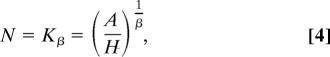giving an explicit definition of a carrying capacity, K_β, as the ability of the population, N, to fill space, A, given individual space requirements, H₀, and spatial organization, β. Note that when β = 1 Eq. 4 gives the linear expectation of carrying capacity, K = A/H. Moreover, Eq. 4 demonstrates how equilibrium abundance is influenced heavily by β.

To consider these implications for hunter–gatherer population dynamics, we note that Eq. 1 implicitly assumes that β = 1. We relax this by substituting Eq. 4 into Eq. 1, yielding

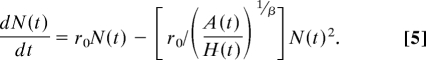Eq. 5 now has the solution N(t) = (A/H₀)^1/β/(1 + c₂e^−rt), where c₂ = [(A/H₀)^1/β/N₀] − 1. Note that Eq. 5 reduces to exponential growth when β = 0 and Eq. 1 when β = 1, demonstrating explicitly how long-term population growth trajectories are affected by intraspecific competition for space. Dividing both sides of Eq. 5 by N gives the per-capita population growth rate (1/N)dN/dt = r(t) = r₀ − α_βN(t), where α_β = r₀/(A/H)^1/β. Therefore, whereas reducing β increases the effective carrying capacity, the population growth rate r(t) also increases as β < 1 reduces the intraspecific competition coefficient (Fig. 3), which has the effect of reducing the per-capita strength of density dependence.

Fig. 3.

Plots of the density-dependent competition model. (Upper) Density-dependent population growth under various strengths of β, Eq. 5; parameters: r₀ = 0.04, K₁ = 500, N₀ = 1. When β = 0, population growth is exponential, and for β = 1, population growth is logistic. (Lower) Isoclines of equilibrium abundance as a function of β.

Population Expansions and Stability

We can now consider the effects of these dynamics on population expansions by spatially extending Eq. 5

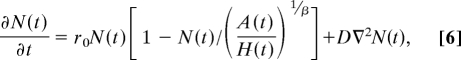where D is the diffusion constant, determined by individual lifetime mobility, and ∇² is the Laplacian operator, representing the diffusion of the population through two-dimensional space as it grows in size through time. The solution to Eq. 6 produces traveling waves of colonists radiating out from a point of origin, moving at a velocity of v = $\sqrt{2r_{0}D}$ across the landscape. Because the velocity v of the wave front is independent of carrying capacity K, reducing β has no effect on the speed of colonization. However, perhaps more importantly, β < 1 results in relatively faster population growth behind the wave front at a rate r(t) = r₀[1 − N(t)/(A/H₀)^1/β] due to the diminished effects of density dependence and the increased carrying capacity. This has important implications for the stability of initial colonizing populations. The leading edge of a colonizing wave is the most demographically unstable part of the colonizing population because of low abundance and density and so is particularly susceptible to environmental perturbations and demographic stochasticity. However, if the population growth rate behind the wave front is rapid, then the population's susceptibility to demographic stochasticity diminishes quickly as sampling effects rapidly become negligible with increasing N. Therefore, although the reduced effects of spatial competition may not necessarily affect the velocity of a colonizing population's wave front, its probability of successfully colonizing new areas is greatly enhanced by the positive effects of β < 1 on both the population growth rate, r(t), and the carrying capacity, K_β.

In nongrowing populations, N(t) = K, stability is often measured by the persistence time, or the expected time to extinction, τ(N), of a population size N starting from equilibrium, K. The probability of extinction in a density-dependent population is finite because the long-term growth rate in a population fluctuating around equilibrium is negative due to the combined effects of demographic and environmental and stochasticity that impact all biological populations (32, 33). In general, the mean time to extinction, τ(N), scales exponentially with carrying capacity, K, so the expected time to extinction of a population at equilibrium abundance scales as τ(K) ∝ e^K (32, 34). Therefore, substituting Eq. 4, we have

Thus, for β < 1, there is a faster than exponential increase in population persistence time, demonstrating the significant payoffs of intraspecific cooperation to long-term population stability. Similarly, we can also consider population stability in terms of the mean return time to equilibrium, δ(K_β), which measures the speed at which a population recovers from a perturbation caused by a population crash (i.e., returns to K). Return time to equilibrium is measured as the reciprocal of the instantaneous growth rate, δ(K_β) = 1/r(t), in a rarefied population of size N(t) (35, 36). Because r(t) = r₀[1 − N(t)/(A/H₀^1/β], β < 1 not only increases the capacity of the population to rebound after a perturbation but also increases its ability to invade new space. Also worth noting here is that later technological and behavioral innovations in human prehistory that led to the development of horticulture and agriculture were essentially methods of increasing the resource supply rate per unit area, R. As such, regional carrying capacities would have increased exponentially, suggesting that the observed increases in population sizes and growth rates coincident with such technological developments may have been simply due to increased resource supply rates rather than changes in fertility, as is often assumed.

Discussion and Conclusions

The model of human ecology we present here explicitly links energy demand and space use with population dynamics by demonstrating how intraspecific cooperation (or competition) for resources affects both equilibrium population sizes and densities. The effective overlap of home ranges increases resource supply rates per unit area (i.e., R ∝ N^1/4) such that the area of the home range used exclusively by individuals decreases as population size increases. In terms of foraging theory, resource supply rates likely increase because of the benefits of cooperative foraging, such as reduced search costs and increased encounter rates. These energetic benefits would favor larger group sizes. Because resources are finite, however, each individual would convey a decreasing rate of benefit, and group sizes would approach an equilibrium determined by resource availability (37). Because resources are both finite and variable through time and space, large populations could not be supported as a single functional unit for an indefinite time, favoring the evolution of fission–fusion population structures, which would allow individuals to maintain the benefits of living in large populations [such as increased flows of biological and cultural information, enhanced innovations rates (38), greater stability, and reduced territorial defense costs (30)], while allowing for flexible responses to changing ecological conditions. Such population structures appear as hierarchical, self-similar social structures where functional groups are nested within higher-level groups, and are a seemingly universal structural property of recent hunter–gatherer populations (27, 39) and other human social networks (40, 41), and are also evident in the social organization of other social mammals (42). Further, because the energetic benefits of larger social groups result in decreased per-capita space use, then not only do group sizes become larger and increasingly structured but they also become denser. Indeed, average hunter–gatherer population sizes are ≈1,000 individuals (27, 31), and because A ∝ N^3/4, they are predicted to be ≈5 times denser and occupy larger areas than a population of solitary mammals of a similar body size. More generally, within-species comparisons between populations of solitary and social mammals show that in carnivores the average home range of social populations is ≈4- to 5-fold greater in size than those of solitary individuals, and in ungulates, ≈15-fold greater (43).

Increases in population sizes have equally important implications for population growth rates. The benefits of cooperation decrease the negative effects of density dependence, increasing per-capita growth rates at any given population size. Note that the model presented here does not predict increases in the intrinsic rate of population growth, r₀, which would imply higher rates of offspring production. This is an important distinction because increased population growth rates can theoretically decrease population stability by increasing the likelihood of a population overshooting its carrying capacity, causing population crash events, or by increasing population growth rates to the extent that they approach chaotic dynamics (35). However, our model predicts neither of these outcomes because the ability of modern human hunter–gatherers to increase resource extraction rates and decrease intraspecific competition does not increase individual fertility per se but simply reduces the strength of density dependence.

These ecological outcomes would have conveyed considerable competitive advantages to modern human populations as they expanded across the globe and encountered both novel environmental conditions and competing hominid species. The ability of modern humans to reduce β below the linear expectation means that once a region was initially colonized populations grew rapidly behind the wave front because of the decreased strength of density dependence, thus greatly reducing the probability of extinction from stochastic events. However, this is not to say that human hunter–gatherer populations were immune to extinction events. Indeed, localized extinction and recolonization events would not have been uncommon in prehistory due to catastrophic natural events and likely played an important role in human evolutionary history (44–47). The model above suggests, rather, that increased population sizes would have reduced the frequency of population extinction caused by stochastic environmental and demographic variation.

Because archaic hominid species also exhibited advanced levels of sociality and technological and behavioral sophistication over other similar-sized mammals, in all likelihood β_archaics < 1. Indeed, before the expansion of modern humans, archaic hominid species had existed continuously throughout southern Eurasia for millennia (6). However, if β_moderns < β_archaics, then invading modern human populations would have had a large competitive advantage over other hominids, resulting in competitive exclusion and ecological replacement. Such increased abilities of modern humans to use space and increase population sizes may have resulted from some combination of broader diets, more flexible material cultures and behaviors, advanced cognition, more effective hunting technologies and behaviors, and increased capacities to share and accumulate information among more individuals and over greater geographic distances. As such, modern humans may have simply out-competed archaic hominid species wherever they were encountered and replaced them locally at rates determined largely by their differential abilities to access available energy.

Cooperative behaviors, including intergenerational transfers of resources and information, hunting, reproduction, and group defense, have been well documented in modern hunter–gatherers (48–50). Because the sublinear scaling coefficient, β, captures the net effects of these cooperative behaviors in mitigating intraspecific competition and density-dependent population regulation, our model framework quantifies their combined effects on population dynamics. These cooperative behaviors reduce intraspecific competition and increase population carrying capacities, per-capita growth rates, and stability. The implication of this model is that the benefits of cooperation mitigated the density-dependent effects of competition and the inherently slow human life history and played a major role in the high rates of population growth and geographic spread as modern humans expanded out of Africa to colonize the globe over the last 50,000 years. Finally, because modern human hunter–gatherers form complex social networks and cooperate to extract and share resources, our model implies that social complexity increases stability in human systems, an issue of ongoing debate in ecology (51, 52). As such, the model presented here also has implications for space use, cooperation, and stability in other social mammals.

References

- 1.Mellars P. Why did modern human populations disperse from Africa ca. 60,000 years ago? A new model. Proc Natl Acad Sci USA. 2006;103:9381–9386. doi: 10.1073/pnas.0510792103. [DOI] [PMC free article] [PubMed] [Google Scholar]
- 2.Osbjorn MP. Has the combination of genetic and fossil evidence solved the riddle of modern human origins? Evol Anthropol. 2004;13:145–159. [Google Scholar]
- 3.Lahr MM, Foley RA. Towards a theory of modern human origins: Geography, demography, and diversity in recent human evolution. Am J Phys Anthropol. 1998;107:137–176. doi: 10.1002/(sici)1096-8644(1998)107:27+<137::aid-ajpa6>3.0.co;2-q. [DOI] [PubMed] [Google Scholar]
- 4.Stringer C. Modern human origins: Progress and prospects. Philos Trans R Soc London Ser B. 2002;357:563–579. doi: 10.1098/rstb.2001.1057. [DOI] [PMC free article] [PubMed] [Google Scholar]
- 5.Hunt TL, Lipo CP. Late colonization of Easter Island. Science. 2006;311:1603–1606. doi: 10.1126/science.1121879. [DOI] [PubMed] [Google Scholar]
- 6.Klein RG. The Human Career: Human Biological and Cultural Origins. Chicago: Univ of Chicago Press; 2009. [Google Scholar]
- 7.Buchanan B, Collard M, Edinborough K. Paleoindian demography and the extraterrestrial impact hypothesis. Proc Natl Acad Sci USA. 2008;105:11651–11654. doi: 10.1073/pnas.0803762105. [DOI] [PMC free article] [PubMed] [Google Scholar]
- 8.Stiner M, Kuhn S. Changes in the ‘connectedness’ and resilience of Paleolithic societies in Mediterranean ecosystems. Hum Ecol. 2006;34:693–712. [Google Scholar]
- 9.Gamble C, Davies W, Pettitt P, Hazelwood P, Richards M. The archaeological and genetic foundations of the European population during the Late Glacial: Implications for ‘agricultural thinking.’. Camb Archaeol J. 2005;15:193–223. [Google Scholar]
- 10.Alonso S, Armour JAL. A highly variable segment of human subterminal 16p reveals a history of population growth for modern humans outside Africa. Proc Natl Acad Sci USA. 2001;98:864–869. doi: 10.1073/pnas.98.3.864. [DOI] [PMC free article] [PubMed] [Google Scholar]
- 11.Liu H, Prugnolle F, Manica A, Balloux F. A geographically explicit genetic model of worldwide human-settlement history. Am J Hum Genet. 2006;79:230–237. doi: 10.1086/505436. [DOI] [PMC free article] [PubMed] [Google Scholar]
- 12.Li JZ, et al. Worldwide human relationships inferred from genome-wide patterns of variation. Science. 2008;319:1100–1104. doi: 10.1126/science.1153717. [DOI] [PubMed] [Google Scholar]
- 13.Fagundes NJR, et al. Statistical evaluation of alternative models of human evolution. Proc Natl Acad Sci USA. 2007;104:17614–17619. doi: 10.1073/pnas.0708280104. [DOI] [PMC free article] [PubMed] [Google Scholar]
- 14.Torroni A, et al. mtDNA analysis reveals a major late Paleolithic population expansion from southwestern to northeastern Europe. Am J Hum Genet. 1998;62:1137–1152. doi: 10.1086/301822. [DOI] [PMC free article] [PubMed] [Google Scholar]
- 15.Torroni A, et al. A signal, from human mtDNA, of postglacial recolonization in Europe. Am J Hum Genet. 2001;69:844–852. doi: 10.1086/323485. [DOI] [PMC free article] [PubMed] [Google Scholar]
- 16.Ramachandran S, et al. Support from the relationship of genetic and geographic distance in human populations for a serial founder effect originating in Africa. Proc Natl Acad Sci USA. 2005;102:15942–15947. doi: 10.1073/pnas.0507611102. [DOI] [PMC free article] [PubMed] [Google Scholar]
- 17.Underhill PA, et al. Y chromosome sequence variation and the history of human populations. Nat Genet. 2000;26:358–361. doi: 10.1038/81685. [DOI] [PubMed] [Google Scholar]
- 18.Brantingham JP, Kerry KW, Krivoshapkin AI, Kuzmin YV. In: Entering America: Northeast Asia and Beringia before the Lasy Glacial Maximum. Madsen DB, editor. Salt Lake City: Univ of Utah Press; 2004. pp. 255–284. [Google Scholar]
- 19.Graf KE. “The good, the bad, and the ugly”: Evaluating the radiocarbon chronology of the middle and late Upper Paleolithic in the Enisei River valley, south-central Siberia. J Archaeol Sci. 36:694–707. [Google Scholar]
- 20.Ricklefs RE, Miller GL. Ecology. New York: Freeman; 2000. [Google Scholar]
- 21.Charnov EL, Berrigan D. Why do female primates have such long lifespans and so few babies? or life in the slow lane. Evol Anthropol. 1993;1:191–194. [Google Scholar]
- 22.Walker R, Hill K, Burger O, Hurtado AM. Life in the slow lane revisited: Ontogenetic separation between chimpanzees and humans. Am J Phys Anthropol. 2006;129:577–583. doi: 10.1002/ajpa.20306. [DOI] [PubMed] [Google Scholar]
- 23.Kaplan HS, Robson AJ. The emergence of humans: The coevolution of intelligence and longevity with intergenerational transfers. Proc Natl Acad Sci USA. 2002;99:10221–10226. doi: 10.1073/pnas.152502899. [DOI] [PMC free article] [PubMed] [Google Scholar]
- 24.Kaplan H, Hill K, Lancaster J, Hurtado AM. A theory of human life history evolution: Diet, intelligence, and longevity. Evol Anthropol. 2000;9:156–185. [Google Scholar]
- 25.Walker RS, Hamilton MJ. Life-history consequences of density dependence and the evolution of human body size. Curr Anthropol. 2008;49:115–122. [Google Scholar]
- 26.Walker RS, Gurven M, Burger O, Hamilton MJ. The trade-off between number and size of offspring in humans and other primates. Proc R Soc London Ser B. 2008;275:827–833. doi: 10.1098/rspb.2007.1511. [DOI] [PMC free article] [PubMed] [Google Scholar]
- 27.Hamilton MJ, Milne BT, Walker RS, Burger O, Brown JH. The complex structure of hunter–gatherer social networks. Proc R Soc London Ser B. 2007;274:2195–2202. doi: 10.1098/rspb.2007.0564. [DOI] [PMC free article] [PubMed] [Google Scholar]
- 28.Hamilton MJ, Milne BT, Walker RS, Brown JH. Nonlinear scaling of space use in human hunter–gatherers. Proc Natl Acad Sci USA. 2007;104:4765–4769. doi: 10.1073/pnas.0611197104. [DOI] [PMC free article] [PubMed] [Google Scholar]
- 29.Stephens DW, Krebs JR. Foraging Theory. Princeton: Princeton Univ Press; 1986. [Google Scholar]
- 30.Jetz W, Carbone C, Fulford J, Brown JH. The scaling of animal space use. Science. 2004;306:266–268. doi: 10.1126/science.1102138. [DOI] [PubMed] [Google Scholar]
- 31.Binford LR. Constructing Frames of Reference. Berkeley, CA: Univ of California Press; 2001. [Google Scholar]
- 32.Lande R. Risks of population extinction from demographic and environmental stochasticity and random catastrophes. Am Nat. 1993;142:911–927. doi: 10.1086/285580. [DOI] [PubMed] [Google Scholar]
- 33.Lande R, Steiner E, Saether B-E. Stochastic Population Dynamics in Ecology and Conservation. Oxford: Oxford Univ Press; 2003. [Google Scholar]
- 34.Renshaw E. Modelling Biological Populations in Time and Space. Cambridge: Cambridge Univ Press; 1990. [Google Scholar]
- 35.May RM, Conway GR, Hassell MP, Southwood TRE. Time delays, density dependence and single-species oscillations. J Anim Ecol. 1974;43:747–770. [Google Scholar]
- 36.Sibly RM, Barker D, Hone J, Pagel M. On the stability of populations of mammals, birds, fish and insects. Ecol Lett. 2007;10:970–976. doi: 10.1111/j.1461-0248.2007.01092.x. [DOI] [PubMed] [Google Scholar]
- 37.Boone JL. In: Evolutionary Ecology and Human Behavior. Smith EA, Winterhalder B, editors. New York: de Gruyter; 1992. pp. 301–338. [Google Scholar]
- 38.Bettencourt LMA, Lobo J, Helbing D, Kühnert C, West GB. Growth, innovation, scaling, and the pace of life in cities. Proc Natl Acad Sci USA. 2007;104:7301–7306. doi: 10.1073/pnas.0610172104. [DOI] [PMC free article] [PubMed] [Google Scholar]
- 39.Zhou WX, Sornette D, Hill RA, Dunbar RIM. Discrete hierarchical organization of social group sizes. Proc R Soc London Ser B. 2005;272:439–444. doi: 10.1098/rspb.2004.2970. [DOI] [PMC free article] [PubMed] [Google Scholar]
- 40.Arenas A, Díaz-Guilera A, Guimerà R. Communication in networks with hierarchical branching. Phys Rev Lett. 2001;86:3196–3199. doi: 10.1103/PhysRevLett.86.3196. [DOI] [PubMed] [Google Scholar]
- 41.Arenas A, Danon L, Díaz-Guilera A, Gleiser PM, Guimerá R. Community analysis in social networks. Euro Phys J B. 2004;38:373–380. [Google Scholar]
- 42.Hill RA, Bentley RA, Dunbar RIM. Network scaling reveals consistent fractal pattern in hierarchical mammalian societies. Biol Lett. 2008;4:748–751. doi: 10.1098/rsbl.2008.0393. [DOI] [PMC free article] [PubMed] [Google Scholar]
- 43.Grant JWA, Chapman CA, Richardson KS. Defended versus undefended home range size of carnivores, ungulates and primates. Behav Ecol Sociobiol. 1992;31:149–161. [Google Scholar]
- 44.Shennan S. Population, culture history, and the dynamics of culture change. Curr Anthropol. 2000;41:811–835. [Google Scholar]
- 45.Eller E, Hawks J, Relethford JH. Local extinction and recolonization, species effective population size, and modern human origins. Hum Biol. 2004;76:689–709. doi: 10.1353/hub.2005.0006. [DOI] [PubMed] [Google Scholar]
- 46.Excoffier L, Schneider S. Why hunter-gatherer populations do not show signs of Pleistocene demographic expansions. Proc Natl Acad Sci USA. 1999;96:10597–10602. doi: 10.1073/pnas.96.19.10597. [DOI] [PMC free article] [PubMed] [Google Scholar]
- 47.Boone JL. Subsistence strategies and early human population history: An evolutionary ecological perspective. World Archaeol. 2002;34:6–25. doi: 10.1080/00438240220134232. [DOI] [PubMed] [Google Scholar]
- 48.Gurven M. To give and to give not: The behavioral ecology of human food transfers. Behav Brain Sci. 2005;27:543–559. [Google Scholar]
- 49.Gurven M, Walker R. Energetic demand of multiple dependents and the evolution of slow human growth. Proc R Soc London Ser B. 2006;273:835–841. doi: 10.1098/rspb.2005.3380. [DOI] [PMC free article] [PubMed] [Google Scholar]
- 50.Hawkes K, O'Connell JF, Jones NGB, Alvarez H, Charnov EL. Grandmothering, menopause, and the evolution of human life-histories. Proc Natl Acad Sci USA. 1998;95:1336–1339. doi: 10.1073/pnas.95.3.1336. [DOI] [PMC free article] [PubMed] [Google Scholar]
- 51.Sole RV, Bascompte J. Self-Organization in Complex Ecosystems. Princeton: Princeton Univ Press; 2006. [Google Scholar]
- 52.May RM. Stability and Complexity in Model Ecosystems. Princeton: Princeton Univ Press; 1973. [PubMed] [Google Scholar]