MACHOS: Markov clusters of homologous subsequences

Abstract

Motivation: The classification of proteins into homologous groups (families) allows their structure and function to be analysed and compared in an evolutionary context. The modular nature of eukaryotic proteins presents a considerable challenge to the delineation of families, as different local regions within a single protein may share common ancestry with distinct, even mutually exclusive, sets of homologs, thereby creating an intricate web of homologous relationships if full-length sequences are taken as the unit of evolution. We attempt to disentangle this web by developing a fully automated pipeline to delineate protein subsequences that represent sensible units for homology inference, and clustering them into putatively homologous families using the Markov clustering algorithm.

Results: Using six eukaryotic proteomes as input, we clustered 162 349 protein sequences into 19 697–77 415 subsequence families depending on granularity of clustering. We validated these Markov clusters of homologous subsequences (MACHOS) against the manually curated Pfam domain families, using a quality measure to assess overlap. Our subsequence families correspond well to known domain families and achieve higher quality scores than do groups generated by fully automated domain family classification methods. We illustrate our approach by analysis of a group of proteins that contains the glutamyl/glutaminyl-tRNA synthetase domain, and conclude that our method can produce high-coverage decomposition of protein sequence space into precise homologous families in a way that takes the modularity of eukaryotic proteins into account. This approach allows for a fine-scale examination of evolutionary histories of proteins encoded in eukaryotic genomes.

Contact: m.ragan@imb.uq.edu.au

Supplementary information: Supplementary data are available at Bioinformatics online. MACHOS for the six proteomes are available as FASTA-formatted files: http://research1t.imb.uq.edu.au/ragan/machos

1 INTRODUCTION

Comparative biology is based on the recognition of homology (Hall, 1994). The concept of homology, originally introduced to characterize anatomical features that have the same function in different animals (Owen, 1843), was subsequently redefined (as ‘homogeny’) in reference to common ancestry (Lankester, 1870). Homology, in the sense of descent with modification from a common ancestor, has long served as the touchstone for comparative molecular biology (Margoliash, 1969; Zuckerkandl and Pauling, 1965a,b), and continues to provide the biological context for comparison of genome sequences and other genome-scale data (Koonin, 2005).

In these molecular and genomic contexts, sets of putatively homologous genes or proteins (‘families’) are typically treated as the fundamental units of analysis (Fitch, 1970; Koonin, 2005). The motivation for this choice is three-fold: genes have long been identified as the units of heritability, and proteins as units of function (hence selectability); and both often exhibit sufficient length (number of nucleotides, codons or amino acids) and variability for rigorous statistical analysis. Consequently, much effort has been invested in recognizing homology among, and delineating families of, genes and proteins. In the absence of sequence data from temporal series of ancestors, sets of sequences are inferred to be homologous if they share a degree of sequence identity or similarity, or exhibit patterns of sequence, that are not held in common with unrelated sequences, e.g. those retrieved by random sampling of a database such as GenBank (Benson et al., 2007) or Protein Data Bank (Berman et al., 2000).

Families are typically delineated via a three-step procedure. First, all sequences within a comprehensive dataset (e.g. the UniProt Knowledgebase, see The Uniprot Consortium, 2007) are compared pairwise using BLAST (Altschul et al., 1990), SSEARCH (Pearson, 1991; Smith and Waterman, 1981) or some other statistical tool, yielding a square matrix of pairwise match scores. Next, scores less significant than some arbitrary threshold are removed from further consideration; if the threshold is chosen well, this eliminates many biologically irrelevant matches but few biologically relevant ones, and greatly reduces computational cost. Finally the remaining sequences are grouped into sets such that the strongest matches are within-set and the weakest between-set; these sets are interpreted as (putatively homologous) families. These steps are often abstracted, explicitly or implicitly, as operations involving graphs, with individual sequences as vertices and pairwise match scores as weighted edges. Indeed, in practice, gene or protein families can actually be delineated by graph partitioning (Enright et al., 2002; Harlow et al., 2004; Krause et al., 2005; Kriventseva et al., 2001; Yona et al., 2000).

Homologs may additionally share other properties including secondary and other higher-order structure, chromosomal location, patterns of intra-molecular interaction, connectivity within pathways and networks, spatial and temporal expression and (as a consequence) cellular function. Investigating the interrelationships among heredity, structure and function has often yielded not only deeper understanding of evolutionary processes, but also biotechnological, biomedical and other practical outcomes.

Genes of morphologically complex eukaryotes are structurally complex. Their exon–intron structure is well-recognized, but additional features are only now becoming apparent, e.g. the presence of sequence motifs for developmentally regulated alternative transcription (Carninci et al., 2005) or miRNA binding (John et al., 2004). The proteins they encode often contain discrete, evolutionarily conserved regions that may fold autonomously, form spatially compact domains, and/or convey specific functions (Bork, 1991; Dorit et al., 1990; Holm and Sander, 1996; Richardson, 1981). These regions may arise from a contiguous stretch of amino acids, or be spatially discontinuous at the primary-sequence level (Jones et al., 1998). In different combinations and arrangements, these subsequences generate novel combinations of folded structure that underlie innovation in protein function, as reflected by the observation that over 80% of metazoan proteins contain two or more domains (Apic et al., 2001).

This complexity creates both conceptual and operational problems for the recognition of homologous families. A set of proteins may share a region of significant primary-sequence similarity but otherwise present no evidence of relatedness; in such cases, we can infer only that the subsequence has descended from a common ancestor (the second step in delineation of families, described above, is intended to reduce the number of false inferences of this type). Worse, a single protein may share different local regions of significant similarity with mutually exclusive partners, i.e. show conflicting patterns of homology. In such cases, it is clearly inappropriate to consider entire proteins (or genes) to constitute the fundamental unit of comparative analysis.

A number of expert-curated databases are available in which protein subsequences, rather than entire proteins, are grouped into putatively homologous families. However, substantial gaps remain in the coverage of known genomes, transcriptomes and other molecular sequences, such that a large fraction of protein sequences remains un-annotated. Various attempts have been made to delineate and classify these domains in a fully automatic manner with the aim to achieve near-complete coverage of protein space. In DOMO, subsequence boundaries are delineated by defining local regions of similarity and reconciling their positions relative to sequence termini (Gracy and Argos, 1998). In ProDom, the shortest sequence in a database is assumed to consist of a single domain; members of that domain family are built up using successive PSI-BLAST searches, and the process iterates until no further sequences can be clustered (Servant et al., 2002). More recently, ADDA decomposes proteins into modules by analysing all-vs-all alignments derived using a global maximum-likelihood model (Heger and Holm, 2003).

Here, we introduce a fully automated method that delineates homologous sequence families by resolving individual proteins into subsequences that we initially treat as fundamental units (i.e. nodes of a graph). Subsequent re-constitution of edges in this graph, followed by Markov clustering, yields sets of putatively homologous subsequence families. Our approach differs from the three other methods cited above in the way that subsequences are constituted, and in the algorithm by which the subsequence similarity graph is resolved into families. We apply this approach to six eukaryotic proteomes, and using an accepted quality score show that our approach performs at least as well as the other fully automated methods (ProDom and ADDA) in recovering protein domains and domain families as annotated in the expert-curated database Pfam. We illustrate the method using the glutamyl/glutaminyl-tRNA synthetase family as an example, and discuss its application in generating homologous subsequence families for phylogenetic analyses.

2 METHODS

2.1 Preparation of protein sequence datasets

Protein sequence and annotation data for human, mouse, rat, fly, worm and yeast were obtained from ENSEMBL release version 42 (Birney et al., 2006). These data include ‘protein variants’ encoded by alternative transcripts and splice variants within a gene locus as defined by the ENSEMBL gene annotation. In order to remove, as efficiently as possible, redundant protein variants (i.e. those encoded by exons that are completely contained within one or more other exons), a strategy was devised to determine the minimal combination of protein variants for which the underlying exons maximally cover that gene locus.

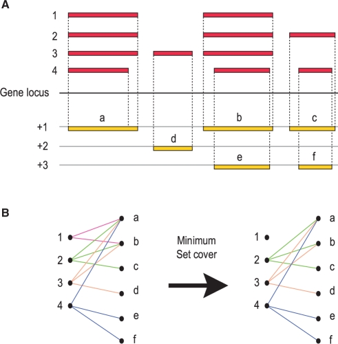
At each gene locus, we define a universe U of all unique nucleotides in all exons transcribed from that locus. Each protein variant is composed of one or more exons, each of which corresponds to a contiguous stretch of nucleotides within U. Therefore each protein variant i∈{1,…,n}, where n is the total number of variants, induces a subset S_i of U, and the union of all S_{i∈{1,…,n}}=U. Our goal was to find the minimum number of sets within {S₁,…,S_n} that maximally cover U. This is a classic set-covering optimization problem, and is known to be NP-hard. We addressed this problem using a greedy algorithm that represents a good polynomial-time approximation (Lund and Yannakakis, 1994). This greedy algorithm iteratively selects S_{i∈{1,…,n}} that cover the maximum number of uncovered nucleotides within U until all nucleotides have been covered (Fig. 1). In our case, we stopped the iteration when the number of uncovered nucleotides fell below 60. For the purposes of the work described here, we consider that below this threshold, the return of additional unique sequence in U is unlikely to justify the increased level of redundancy; other thresholds, however, may be more appropriate in other contexts.

Fig. 1.

Selection of protein variants to represent each gene locus. (A) Shown is a hypothetical gene locus where alternative transcription or splicing events result in four protein variants numbered from 1 to 4. The exons of each protein variant map onto the gene locus in one of three different reading frames (+1/+2/+3), resulting in regions a–f. Note that regions b and e overlap the same stretch of sequence in the gene locus but their translated protein sequence may be different as they are in different reading frames. (B) Each protein variant thus associates with one or more of regions (a–f), as represented in the bipartite graph. A greedy algorithm was then used (see Methods) to find the minimum set of protein variants that maximizes coverage of regions a–f.

The description in the paragraph immediately above ignores the issue of alternative reading frames. Each local region in the gene locus can potentially encode three different substrings of amino acids, and the protein variants that contain them can find different sets of match partners. Therefore in the actual implementation, each nucleotide in U was allowed up to three unique instances, one in each (local) coding frame.

To reduce computational load, where sequences exhibited 100% identity (whether inter- or intra-specifically) one representative was selected at random to serve as a placeholder through the subsequent comparison and graph partitioning operations. The other copies (with the corresponding annotation) were then reinstated into the final subsequence family classification.

2.2 Detection of homologous sequences and alignments

Pairwise putative homologs were detected by an all-vs-all similarity search using the Smith–Waterman algorithm as implemented in SSEARCH (Pearson, 1991; Smith and Waterman, 1981). We used SSEARCH parameters (a BLOSUM65 substitution matrix generated using the BLOCKS 13+ database, gap penalty of −12, and gap extension of −1) that have been shown to achieve good accuracy in similarity detection as evidenced by their ability to retrieve SCOP families (Price et al., 2005), along with an expectation value cut-off of 0.01. However, since SSEARCH identifies only the single best local alignment between any two sequences, pairwise LALIGN (Huang et al., 1990) with the same SSEARCH parameters was used in a subsequent step to identify other regions (if any) of significant similarity that do not overlap with the top local alignment.

2.3 Delineation of subsequences

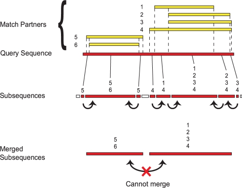
For each query protein sequence, there may exist a set of local pairwise alignments to one or more other sequences (match partners), whether inter- or intra-specifically. At any defined threshold, each of these pairwise alignments extends through a discrete local region in both query and target sequence and, together, these regions cover the query sequence to a greater or lesser extent. In this way, each query sequence becomes partitioned into non-overlapping subsequences, with all residues within a subsequence having a common set of match partners. If there is an adjacent subsequence, all residues therein will likewise share a common (but different, i.e. not fully identical) set of match partners (Fig. 2). Each subsequence can be represented as a node in a similarity graph.

Fig. 2.

Subsequence delineation and merging procedure. In order to demonstrate how subsequences are generated, shown is a hypothetical query protein sequence with regions of local similarity to a set of target proteins (or match partners) labelled 1–6. On this basis, the query protein sequence is divided into non-overlapping subsequences such that each individual subsequence matches a set of partners (indicated at the top of each subsequence) that is different from the set matched by its adjacent subsequences. Some of these adjacent subsequences are merged (indicated by arrows) if they do not match mutually exclusive partners. Merging occurs iteratively until no further adjacent subsequences can be merged. At the end of this process, the query protein is divided into regions which show different signals of homology that are indicative of a modular composition.

However, delineating subsequences by forcing all their residues to share a common set of match partners may be too restrictive, as short subsequences were frequently defined at subsequence boundaries owing e.g. to alignment artifacts. We therefore merged adjacent subsequences if they satisfied two conditions: (a) the match partners of one of the subsequences form a complete subset of the other and (b) at least one of the subsequences is <20 residues in length. The resulting merged subsequence was then defined to have the same set of match partners as the longer of the original two subsequences. Successive rounds of merging were applied until no further adjacent subsequences could be merged. This has the effect of restricting the proliferation of weakly supported, information-poor subsequence sets.

2.4 Construction of the subsequence similarity graph

We next generated a graph in which each node represents one of our (possibly merged) subsequences, and the edges represent the pairwise weighted sequence similarity. An edge is drawn between two subsequences if (a) one subsequence occurs in its entirety within their pairwise local alignment or (b) the two subsequences share a region of sequence similarity that covers 50% or more of either subsequence. The weight of an edge is given by −logE where E is the expectation value of the local alignment as already calculated by LALIGN.

2.5 Markov clustering of subsequence similarity graph

The subsequence similarity graph first had to be divided into coarse disjoint sets, because the MCL software demanded excessive memory when the entire graph was used as input. To accomplish this, we generated and coarsely partitioned a protein-similarity graph (see next section), then mapped the merged subsequences onto its disjoint partitions, thereby partitioning the subsequence graph into the same number of coarse disjoint sets. Only those edges that exist within each disjoint set were retained. We then ran MCL on each disjoint set using a range of inflation parameter values (1.2, 1.6, 2.0 and 2.4) that determine granularity of the clustering. As there can be no similarity relationships between disjoint sets, the results from all disjoint sets were subsequently collated into a classification of subsequence families (‘Markov Clusters of Homologous Subsequences’, MaCHoS or more simply, MACHOS) at each inflation parameter value.

2.6 Protein-similarity graph

The protein-similarity graph used in the previous section was generated using complete protein sequences as vertices. An edge was drawn between a pair of vertices if the E-value of their pairwise SSEARCH match was better than 0.01 (above), and each edge was weighted by its SSEARCH E-value. This graph was then coarsely partitioned using the Markov clustering software MCL, obtained from http://micans.org/mcl/src (van Dongen, 2000), with inflation parameter I=1.2.

2.7 Quality assessment using Pfam domain families

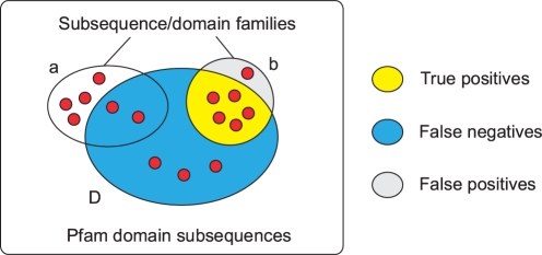
We mapped the reference classification of Pfam domains, as annotated by the ENSEMBL database (Birney et al., 2006), onto our subsequences, yielding clusters of subsequences that correspond to the Pfam domain families. In this process, every Pfam domain maps to at least one subsequence, while the converse is not true: some subsequences are not assigned to any Pfam domain. We then examined the extent to which the subsequence families delineated in this way (‘Pfam subsequence families’, PSFs) overlap with the MACHOS generated above. To help ensure that only related families contribute to the assessment of quality, we include a MACHOS in the analysis only if at least 50% of its members lie within a single PSF. Where a single PSF is overlapped by one or more such MACHOS (Fig. 3), we define three types of subsequences in the union set: true positives (TP) (subsequences in the PSF–MACHOS intersection), false positives (FP) (in the MACHOS but not the PSF) and false negatives (FN) (in the PSF but not the MSF). For each PSF we calculate the quality score Q as:

(1)

Fig. 3.

A graphical representation of how quality scores are derived when comparing a subsequence family classification scheme with a reference classification such as Pfam. Red circles represent individual subsequences and the set D delineates all subsequences that belong to the same Pfam domain family. Only those subsequence families (e.g. MACHOS) with ≥50% of their members overlapping the Pfam domain family (set b in this example, but not set a) are used in calculating the quality score based on the number of subsequences in the TP (yellow), FN (blue) and FP (grey) regions.

However, there exists the possibility that our classification scheme is too granular, i.e. that we have many small MACHOS overlapping a single PSF; this would generate a misleadingly high quality score. Such cases can be penalized by the following:

(2)

As previously suggested (Yona et al., 1999), this measure may be over-conservative. Since the coverage of our protein space by Pfam domains is not complete, there may be well valid members within our MACHOS that are not annotated by Pfam, and this will result in over-estimation of our FP rate. We account for this by calculating an upper bound on our quality score by setting the FP rate to 0 in the Q_adjusted equation above. This yields a new measure Q_upper

(3)

The true quality score for a particular PSF probably lies between Q_adjusted and Q_upper.

2.8 Comparison with ADDA and ProDom

Domain-family annotation and FASTA-formatted sequences of source proteins were obtained from http://ekhidna.biocenter.helsinki.fi/downloads/adda for ADDA (Heger and Holm, 2003) and from http://prodom.prabi.fr for ProDom version 2005.1 (Bru et al., 2005). Full-length protein sequences were included with our dataset of 125 008 non-redundant proteins into a single FASTA file, and the common intersection of source protein data among the three datasets was found using Warren Gish's nrdb (http://blast.wustl.edu/pub/nrdb/nrdb2).

To compare the performance of ADDA, ProDom and our approach with respect to Pfam domains, we delineated subsequences within this common set of protein sequences and classified them into families using domain annotations in the file domains.fasta for ADDA, and prodom.srs for ProDom. These subsequence families were then treated in the same manner as our MACHOS in the calculation of quality scores, as described above.

3 RESULTS

3.1 Detection of homologous proteins

We obtained 162 349 protein sequences annotated by ENSEMBL for human, mouse, rat, fly, worm and yeast (Birney et al., 2006). A greedy algorithm for set-covering optimization was employed to achieve efficient coverage of protein-coding regions. We intended this approach to ensure that sequences encoded by most, if not all, exons are represented in our protein space (Fig. 1), and with these data we found that only 0.004% of all exons fail to be represented. However, protein variants encoded by the same ENSEMBL gene locus are kept if they contain mutually exclusive sequence information (until iteration is stopped: see Methods). Further removal of redundancy by collapsing sequences that are 100% identical into one representative sequence yielded a protein dataset with 125 008 members, corresponding to 99.91% of the underlying exonic sequence.

This protein dataset was used as input to an all-vs-all SSEARCH similarity detection pipeline using an E-value cut-off of 0.01. There were 12 229 proteins which found no significant match. Among the remaining 112 779 proteins, SSEARCH identified 11 986 329 pairwise local alignments with significant similarity. However, SSEARCH identifies only the single best region of similarity, and homologous proteins can potentially share multiple regions of similarity in the same or different order. Therefore we subsequently used LALIGN to re-analyse the sequence pairs showing SSEARCH matches, and identified a further 791 pairwise local alignments.

3.2 Delineation of subsequences and Markov clustering into families

The 125 008 proteins were resolved into 1 049 488 subsequences using our delineation and merging procedure (see Methods). Our methodology examines the local alignments of each protein and finds stretches of residues (subsequences), which are aligned to a consistent set of target proteins (Fig. 2). At the end of the process, a boundary is accepted between adjacent subsequences if they match mutually exclusive sets of target proteins, or if the match sets are different (i.e. not fully identical) and both subsequences are at least 20 residues in length. This has the effect of splitting individual nodes of a complete-protein-similarity graph into multiple sub-nodes where the evidence indicates a connectivity difference between or among sub-nodes.

In this new graph, in which all new (sub-) nodes represent subsequences, it is now necessary to reconstitute edges. We draw an edge to represent the alignment between two sequences or subsequences in different proteins. Some of these edges will have the same meaning as before (i.e. between pairs of proteins not resolved into subsequences), but many will now represent local alignments between subsequences. The edges are again weighted by the E-value of the match (see Methods).

Due to memory requirements, the entire subsequence graph was too large to be used as input into the Markov clustering software MCL (van Dongen, 2000). To circumvent this problem, we first partitioned the subsequence graph into disjoint subgraphs. We did this by partitioning the protein-similarity graph into coarse-grained families, then mapping the subsequences and edges back onto these families (see Methods). While this process removed 22 059 168 (7.64%) of the total number of edges from the subsequence graph (i.e. those mapping between the coarse-grained families), these tend to have larger (less-significant) E-values; overall, 97.67% of the total edge weight from the original subsequence graph was retained. Subsequent application of Markov clustering independently to these disjoint graphs, and collation of the resulting clusters, yielded MACHOS for our protein dataset.

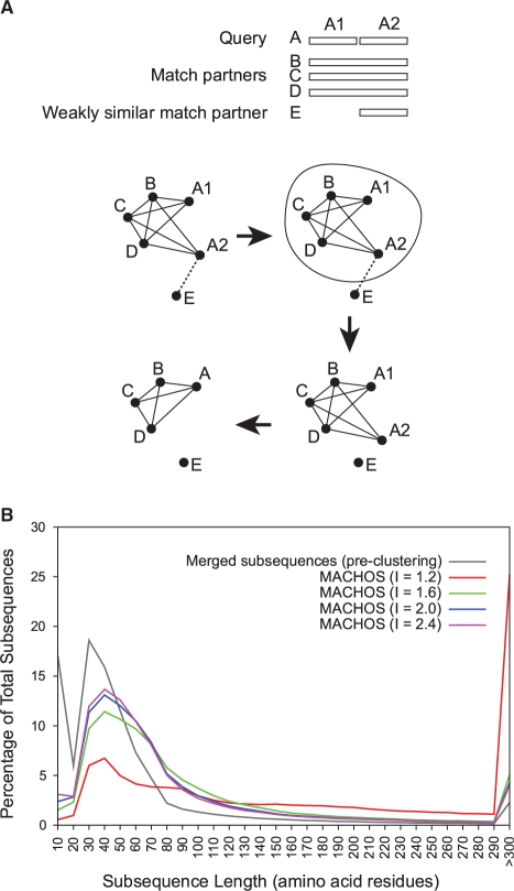
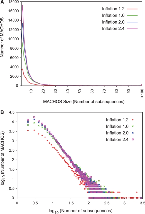
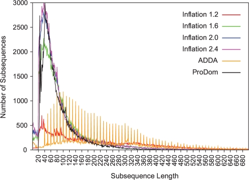
Throughout the above process the possibility has remained that protein sequences might be needlessly split into subsequences owing to alignment artifacts or to the inclusion of non-homologous sequences (Fig. 4A); indeed at this point we observed 257 400–641 343 such instances, depending on granularity of clustering. We merged such adjacent subsequences within the same MACHOS, treating them as a single subsequence throughout subsequent analyses. As expected, as the Markov inflation parameter was increased and the clusters became finer-grained, the subsequences in the final set of MACHOS become shorter in length (Fig. 4B), and the number of subsequence families increases (Fig. 5A). However, all family size distributions are linear in a log–log plot (Fig. 5B), indicating a common theme of many small and few large families, in keeping with other known domain or protein families (Kunin et al., 2005).

Fig. 4.

(A) A hypothetical situation in which the query protein A is fragmented into A1 and A2 by the inclusion of a match partner E that is only weakly similar (perhaps non-homologous) to part of A. The similarity graph shows strong links among the real homologs (A, B, C and D) and a weak link between A2 and E. Subsequent Markov clustering effectively cuts the weak link and results in one MACHOS containing both A1 and A2, which are then joined and treated as a single subsequence, correcting for the initial over-fragmentation. (B) The distributions of subsequence lengths, before and after subsequences are clustered into MACHOS at different granularities (indicated by coloured lines), are shown with a bin size of 10 residues. Although the underlying data are discrete points, we have represented the data as smooth coloured lines to aid visual analysis.

Fig. 5.

(A) The distributions of MACHOS sizes at different inflation values (indicated by coloured lines) are shown. The smooth coloured lines connect underlying data points and are used to aid visual analysis. (B) The same data shown as a log–log plot.

3.3 Validation with Pfam

To estimate the quality of our subsequence families, we compared our classification of protein subsequences with Pfam, a well-established expert-curated domain database (Finn et al., 2006). The evaluation methodology as proposed by Yona et al. (1999) was adapted to produce quality scores for our clustering results at different inflation parameters (see Methods).

Quality scores reflecting how well our clusters correspond to Pfam domain families are shown in Table 1. It is notable that MACHOS quality is not greatly affected by granularity except at I=1.2, where MACHOS are largest (Table 1). A subsequence contributes to the quality score only if it is present in the union of an MACHOS with a PSF that overlaps it by ≥50% (see Methods). Given a fixed size distribution of PSFs, large MACHOS are less frequently overlapped to this extent, and this is reflected in the relatively large number (1003) of PSFs that do not overlap a MACHOS by ≥50% at I=1.2 (Table 2). For the PSFs that do overlap one or more MACHOS, most overlap three or fewer MACHOS (Table 2), and relatively high numbers of FN were observed, leading to a low overall quality score (Table 1). In contrast, more PSFs overlap MACHOS generated at I≥1.6, and the corresponding quality scores are markedly higher (Table 2). Our results suggest that the MACHOS generated at I≥1.6 are in better agreement with PSFs.

Table 1.

Quality assessment of subsequence clusters using Pfam as a reference

	Inflation	Clusters	TP %	FP %	FN %	Qadjusted%	Qupper%	Non-overlapping MACHOS
MACHOS (complete set)	1.2	19 697	63.55	17.02	19.44	61.57	76.24	14 865
	1.6	49 565	71.24	17.56	11.20	67.43	82.24	31 297
	2.0	65 534	73.01	16.96	10.03	68.19	82.42	32 257
	2.4	77 415	73.96	16.78	9.26	68.42	82.43	29 638
MACHOS (subset)	1.2	16 923	61.91	19.47	18.63	57.79	74.21	12 000
	1.6	40 044	67.68	20.06	12.26	59.83	75.63	25 396
	2.0	51 372	68.97	19.56	11.47	59.33	74.41	24 526
	2.4	59 260	69.86	19.46	10.68	58.87	73.62	20 051
ADDA		42 977	62.82	17.19	20.13	55.01	68.85	36 254
ProDom		98 863	62.96	10.05	26.99	43.46	48.66	68 735

MACHOS (subset) refers to the subset of our subsequence families originating from the set of protein sequences that overlaps those used and annotated by ADDA and Prodom. Abbreviations: TP = true positives; FP = false positives; FN = false negatives.

Table 2.

Number of PSFs which are individually overlapped by different numbers of subsequence families

		Number of subsequence families overlapping a PSF by ≥50% of subsequence members
	Method	0	1	2	3	4	5	6–10	>10
Number of PSFs	MACHOS I=1.2	1003	1378	561	218	78	50	72	45
	MACHOS I=1.6	345	1115	689	354	212	166	291	233
	MACHOS I=2.0	270	1019	661	361	207	171	376	340
	MACHOS I=2.4	240	967	626	357	217	169	420	409
	MACHOS I=1.2	1061	1298	498	202	66	41	54	32
	MACHOS I=1.6	398	1102	626	351	202	147	252	174
	MACHOS I=2.0	298	1030	617	356	195	157	343	256
	MACHOS I=2.4	267	971	603	363	188	167	376	317
	ADDA	644	1381	548	253	133	81	123	89
	ProDom	57	433	461	452	318	251	659	621

The top half of the table contains numbers derived from the MACHOS classification on the complete protein dataset. The bottom half shows the numbers calculated from different classification methods, which used a common subset of the complete protein dataset as input (see Methods).

Quality scores for MACHOS generated at I≥1.6 do not differ greatly, although they increase slightly at higher inflation values (Table 1). However, MACHOS generated at higher inflation values are much more granular, yielding shorter subsequences in larger numbers of families (Fig. 4B). In this sense MACHOS generated at I=1.6 are a good compromise between accuracy and the need to avoid over-fragmentation into short subsequences.

3.4 Comparison with ADDA and ProDom

In order to compare our MACHOS with the domain or module families produced by other fully automated classification schemes, a set of 58 985 protein sequences was identified as the intersection of source data among ADDA, ProDom and our own dataset of 125 008 non-redundant proteins (see Methods). The following comparative analyses are based on different classifications of this intersection dataset.

The length distributions of our merged subsequences, ADDA modules and ProDom domains within non-singleton families are shown in Figure 6. Our subsequences generally decrease in length as the granularity of our clustering increases (i.e. as our MACHOS become, on average, smaller). The length distribution of ProDom domains is similar to that of our subsequences when we generate MACHOS at I=2.0 and 2.4. In general, ADDA proposes longer module lengths, with interesting spikes in the count at lengths that are exact multiples of 10; to our knowledge this has not been previously documented, and presumably arises from a rounding operation inherent in the ADDA method.

Fig. 6.

The distributions of subsequence/domain lengths in non-singleton families are shown using data from six family classification schemes (indicated by coloured lines): MACHOS generated at different inflation values from 1.2 to 2.4, ADDA (orange line) and ProDom (black line). The distributions of subsequences >700 residues in length are not shown as they form a long tail. The continuous coloured lines connect underlying data points and are used to aid visual analysis.

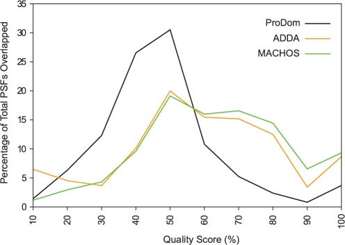
Quality scores for the different clusterings, again using the PSFs as the reference classification, were calculated using the same method and criteria (see Methods) and are shown in Table 1. Again, MACHOS show notably lower quality scores when generated at I=1.2 than at higher granularity, and the same trend is observed in numbers of non-overlapping PSFs. The mean quality scores of our MACHOS generated at any inflation value are higher than those from ADDA and ProDom. On a finer level, we compared the distribution of PSFs that overlap MACHOS or ADDA/ProDom domain families by 50% across different quality scores (Fig. 7). The relatively low mean quality score of ProDom domain families is apparent as 87% of overlapped PSFs achieved quality scores of <60%. On the other hand, larger proportions of PSFs overlapping ADDA domain families and MACHOS achieved higher quality scores compared to ProDom. However, the PSF coverage of ADDA domain families is lower than that of MACHOS, reflected by the relatively larger number of non-overlapping PSFs (Table 2). The results indicate that our MACHOS achieve better coverage, and are more congruent with PSFs, compared with the output of the other methods we consider.

Fig. 7.

The distribution of quality scores achieved by different subsequence/domain family classification methods (indicated by coloured lines) are shown with a bin size of 10%. The coloured lines connect underlying data points and are used to aid visual analysis.

3.5 Non-overlapping Pfam families

Whereas our concern so far has been the extent of overlap and agreement between PSFs and MACHOS, we now focus on the PSFs that fail to overlap any MACHOS by 50%. At I=1.6 there are 345 of these non-overlapping PSFs (Table 2); these PSFs are generally small (Supplementary Table 1), and collectively represent only 2.9% of the total residues covered by all PSFs.

Interestingly, the number of non-overlapping PSFs is significantly less for ProDom than for any of these other approaches. This highlights a potential bias, in that much of the Pfam domain family annotation, namely Pfam-B, was derived from ProDom families in the first place (Bateman et al., 2004). Intriguingly, however, quality scores of the ProDom families are the lowest among all these classification schemes, even when FP are excluded from consideration. The reason for this phenomenon appears to be that ProDom families are more granular than MACHOS or ADDA domain families. Compared to other methods, ProDom generated the highest number of families (Table 1). As the granularity of subsequence/domain families increases, the number of non-overlapping PSFs decreases. This trend can also be observed in MACHOS, where the number of non-overlapping PSFs falls with increasing inflation value or granularity (Table 1). The consequence of having such a high coverage of PSFs is that individual PSFs tend to overlap higher numbers of subsequence/domain families, which is especially true in the case of ProDom (Table 2). Since the quality score favours smaller numbers of subsequence/domain families that are overlapped by individual PSFs, the quality scores achieved by ProDom are generally lower as a result.

3.6 Example of subsequence families within a ‘protein’ family

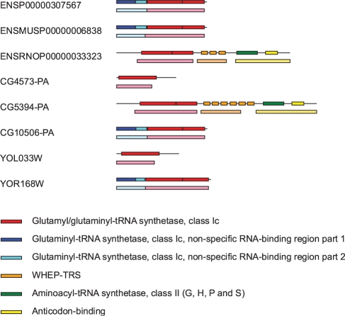
We illustrate our method using a group of proteins in our dataset which contain the glytamly/glutaminyl-tRNA synthetase domain as annotated by Pfam (Fig. 8). One of our MACHOS generated at inflation value of 1.6 was found to delineate independently all occurrence of this domain within the dataset. More importantly, it is apparent that subsets of this group of proteins also share other domains. For example, ENSRNOP00000033323 and CG5394-PA both contain the WHEP-TRS, aminoacyl-tRNA synthetase and anticodon-binding domains. In this case, one MACHOS uncovered the WHEP-TRS domains, and another MACHOS uncovered the aminoacyl-tRNA synthetase and anticodon-binding domains. This is an example where multiple Pfam domains may be found within the same MACHOS; in our experience, this occurs when the domains are always found together in the same order within the protein dataset. Effectively, the combination of domains merely becomes a single ‘unit’ in our approach. Another example is the MACHOS uncovering the two parts of the glytaminyl-tRNA synthetase non-specific RNA-binding domain which occur in the same order in four of the eight proteins as mentioned.

Fig. 8.

The family of proteins that contain the glutamyl/glutaminyl-tRNA synthetase domain (shown in red). Each protein is shown with its ENSEMBL translation ID and a horizontal line representing the full-length protein sequence. Coloured rectangles drawn on top of horizontal lines are Pfam domain annotations and the different colours refer to different domain families as indicated. Coloured rectangles beneath horizontal lines represent subsequences delineated by our method and those with the same colour belong to a distinct MACHOS. All lines and rectangles are drawn to scale with respect to the length of the protein sequences.

4 DISCUSSION

We have developed a method for the automated delineation of homologous subsequence families. This method first resolves proteins into sensible fragments which can show conflicting homology signals indicative of multi-domain organization. Then the elegant Markov clustering algorithm, previously used in clustering complete proteins into families, is employed to resolve more-strongly connected clusters of these fragments that we interpret as putatively homologous subsequence families. By analysis of protein sequences from six eukaryotic proteomes, we demonstrate that our method can automatically delineate subsequence families that are akin to Pfam domain families. Our approach differs from existing methods in the approach by which subsequences are constituted, and the Markov clustering approach to resolution of subsequence families. It is difficult to draw direct comparisons on the merits and shortfalls of all the methods, as they take quite different approaches to resolve subsequence/domain families. But the simplicity and flexbility of our approach have produced subsequence families that achieve better coverage and are more congruent with Pfam domain families, compared to ADDA and ProDom.

The most computationally demanding parts of the method are (a) inference of homology using SSEARCH and LALIGN and (b) Markov clustering of the subsequence homology graph. Together they required ≈ 13 679 h of CPU time for completion. We have thus been prevented from carrying out the same analyses on larger numbers of proteomes. However, parallel implementation of some of these algorithms already exists (e.g. parallel SSEARCH) or is being developed (e.g. parallel Markov clustering: K. Burrage and A. Bustamam, personal communication), which should enable our pipeline to handle much larger protein datasets.

It is important to note that while our families show good correspondence to trusted, manually curated Pfam domain families, our objective has not been to retrieve families of structural domains, but rather to assemble sets of full- or partial-length protein homologs that have been delineated with sufficient resolution (both along the sequence co-ordinates, and among species) for high-quality application in comparative genomic or proteomic analyses including selection of model organisms, interolog-based inference and phylogenetic analysis.

Funding: This work was supported by Australian Research Council grant CE0348221.

Conflict of Interest: none declared.

REFERENCES

- Altschul SF, et al. Basic local alignment search tool. J. Mol. Biol. 1990;215:403–410. doi: 10.1016/S0022-2836(05)80360-2. [DOI] [PubMed] [Google Scholar]
- Apic G, et al. Domain combinations in archaeal, eubacterial and eukaryotic proteomes. J. Mol. Biol. 2001;310:311–325. doi: 10.1006/jmbi.2001.4776. [DOI] [PubMed] [Google Scholar]
- Bateman A, et al. The Pfam protein families database. Nucleic Acids Res. 2004;32:D138–D141. doi: 10.1093/nar/gkh121. [DOI] [PMC free article] [PubMed] [Google Scholar]
- Benson DA, et al. GenBank. Nucleic Acids Res. 2007;35:D21–D25. doi: 10.1093/nar/gkl986. [DOI] [PMC free article] [PubMed] [Google Scholar]
- Berman HM, et al. The Protein Data Bank. Nucleic Acids Res. 2000;28:235–242. doi: 10.1093/nar/28.1.235. [DOI] [PMC free article] [PubMed] [Google Scholar]
- Birney E, et al. Ensembl 2006. Nucleic Acids Res. 2006;34:D556–D561. doi: 10.1093/nar/gkj133. [DOI] [PMC free article] [PubMed] [Google Scholar]
- Bork P. Shuffled domains in extracellular proteins. FEBS Lett. 1991;286:47–54. doi: 10.1016/0014-5793(91)80937-x. [DOI] [PubMed] [Google Scholar]
- Bru C, et al. The ProDom database of protein domain families: more emphasis on 3D. Nucleic Acids Res. 2005;33:D212–D215. doi: 10.1093/nar/gki034. [DOI] [PMC free article] [PubMed] [Google Scholar]
- Carninci P, et al. The transcriptional landscape of the mammalian genome. Science. 2005;309:1559–1563. doi: 10.1126/science.1112014. [DOI] [PubMed] [Google Scholar]
- Dorit RL, et al. How big is the universe of exons? Science. 1990;250:1377–1382. doi: 10.1126/science.2255907. [DOI] [PubMed] [Google Scholar]
- Enright AJ, et al. An efficient algorithm for large-scale detection of protein families. Nucleic Acids Res. 2002;30:1575–1584. doi: 10.1093/nar/30.7.1575. [DOI] [PMC free article] [PubMed] [Google Scholar]
- Finn RD, et al. Pfam: clans, web tools and services. Nucleic Acids Res. 2006;34:D247–D251. doi: 10.1093/nar/gkj149. [DOI] [PMC free article] [PubMed] [Google Scholar]
- Fitch WM. Distinguishing homologous from analogous proteins. Syst. Zool. 1970;19:99–113. [PubMed] [Google Scholar]
- Gracy J, Argos P. Automated protein sequence database classification. II. Delineation of domain boundaries from sequence similarities. Bioinformatics. 1998;14:174–187. doi: 10.1093/bioinformatics/14.2.174. [DOI] [PubMed] [Google Scholar]
- Hall BK. Homology. The hierarchical basis of comparative biology. San Diego: Academic Press; 1994. [Google Scholar]
- Harlow TJ, et al. A hybrid clustering approach to recognition of protein families in 114 microbial genomes. BMC Bioinformatics. 2004;5:45. doi: 10.1186/1471-2105-5-45. [DOI] [PMC free article] [PubMed] [Google Scholar]
- Heger A, Holm L. Exhaustive enumeration of protein domain families. J. Mol. Biol. 2003;328:749–767. doi: 10.1016/s0022-2836(03)00269-9. [DOI] [PubMed] [Google Scholar]
- Holm L, Sander C. Mapping the protein universe. Science. 1996;273:595–603. doi: 10.1126/science.273.5275.595. [DOI] [PubMed] [Google Scholar]
- Huang XQ, et al. A space-efficient algorithm for local similarities. Comput. Appl. Biosci. 1990;6:373–381. doi: 10.1093/bioinformatics/6.4.373. [DOI] [PubMed] [Google Scholar]
- John B, et al. Human microRNA targets. PLoS Biol. 2004;2:e363. doi: 10.1371/journal.pbio.0020363. [DOI] [PMC free article] [PubMed] [Google Scholar]
- Jones S, et al. Domain assignment for protein structures using a consensus approach: characterization and analysis. Protein Sci. 1998;7:233–242. doi: 10.1002/pro.5560070202. [DOI] [PMC free article] [PubMed] [Google Scholar]
- Koonin EV. Orthologs, paralogs, and evolutionary genomics. Annu. Rev. Genet. 2005;39:309–338. doi: 10.1146/annurev.genet.39.073003.114725. [DOI] [PubMed] [Google Scholar]
- Krause A, et al. Large scale hierarchical clustering of protein sequences. BMC Bioinformatics. 2005;6:15. doi: 10.1186/1471-2105-6-15. [DOI] [PMC free article] [PubMed] [Google Scholar]
- Kriventseva EV, et al. Clustering and analysis of protein families. Curr. Opin. Struct. Biol. 2001;11:334–339. doi: 10.1016/s0959-440x(00)00211-6. [DOI] [PubMed] [Google Scholar]
- Kunin V, et al. The properties of protein family space depend on experimental design. Bioinformatics. 2005;21:2618–2622. doi: 10.1093/bioinformatics/bti386. [DOI] [PubMed] [Google Scholar]
- Lankester ER. On the use of the term homology in modern zoology. Ann. Mag. Nat. Hist. 1870;6:34–43. [Google Scholar]
- Lund C, Yannakakis M. On the hardness of approximating minimization problems. J. ACM. 1994;41:960–981. [Google Scholar]
- Margoliash E. Homology: a definition. Science. 1969;163:127. doi: 10.1126/science.163.3863.127. [DOI] [PubMed] [Google Scholar]
- Owen R. Lectures on the comparative anatomy and physiology of the invertebrate animals, delivered at the Royal College of Surgeons, I 1843. London: Longmans Brown Green & Longmans; 1843. p. 379. [Google Scholar]
- Pearson WR. Searching protein sequence libraries: comparison of the sensitivity and selectivity of the Smith-Waterman and FASTA algorithms. Genomics. 1991;11:635–650. doi: 10.1016/0888-7543(91)90071-l. [DOI] [PubMed] [Google Scholar]
- Price GA, et al. Statistical evaluation of pairwise protein sequence comparison with the Bayesian bootstrap. Bioinformatics. 2005;21:3824–3831. doi: 10.1093/bioinformatics/bti627. [DOI] [PubMed] [Google Scholar]
- Richardson JS. The anatomy and taxonomy of protein structure. Adv. Protein Chem. 1981;34:167–339. doi: 10.1016/s0065-3233(08)60520-3. [DOI] [PubMed] [Google Scholar]
- Servant F, et al. ProDom: automated clustering of homologous domains. Brief. Bioinform. 2002;3:246–251. doi: 10.1093/bib/3.3.246. [DOI] [PubMed] [Google Scholar]
- Smith TF, Waterman MS. Identification of common molecular subsequences. J. Mol. Biol. 1981;147:195–197. doi: 10.1016/0022-2836(81)90087-5. [DOI] [PubMed] [Google Scholar]
- The Uniprot Consortium. The Universal Protein Resource (UniProt) Nucleic Acids Res. 2007;35:D193–D197. doi: 10.1093/nar/gkl929. [DOI] [PMC free article] [PubMed] [Google Scholar]
- van Dongen S. Graph Clustering by Flow Simulation. Utrecht: University of Utrecht; 2000. PhD thesis. [Google Scholar]
- Yona G, et al. ProtoMap: automatic classification of protein sequences, a hierarchy of protein families, and local maps of the protein space. Proteins. 1999;37:360–378. [PubMed] [Google Scholar]
- Yona G, et al. ProtoMap: automatic classification of protein sequences and hierarchy of protein families. Nucleic Acids Res. 2000;28:49–55. doi: 10.1093/nar/28.1.49. [DOI] [PMC free article] [PubMed] [Google Scholar]
- Zuckerkandl E, Pauling L. Evolutionary divergence and convergence in proteins. In. In: Bryson V, Vogel HJ, editors. Evolving Genes and Proteins. New York: Academic Press; 1965a. pp. 97–166. [Google Scholar]
- Zuckerkandl E, Pauling L. Molecules as documents of evolutionary history. J. Theor. Biol. 1965b;8:357–366. doi: 10.1016/0022-5193(65)90083-4. [DOI] [PubMed] [Google Scholar]
Associated Data
This section collects any data citations, data availability statements, or supplementary materials included in this article.