Estimating true evolutionary distances under the DCJ model

Abstract

Motivation: Modern techniques can yield the ordering and strandedness of genes on each chromosome of a genome; such data already exists for hundreds of organisms. The evolutionary mechanisms through which the set of the genes of an organism is altered and reordered are of great interest to systematists, evolutionary biologists, comparative genomicists and biomedical researchers. Perhaps the most basic concept in this area is that of evolutionary distance between two genomes: under a given model of genomic evolution, how many events most likely took place to account for the difference between the two genomes?

Results: We present a method to estimate the true evolutionary distance between two genomes under the ‘double-cut-and-join’ (DCJ) model of genome rearrangement, a model under which a single multichromosomal operation accounts for all genomic rearrangement events: inversion, transposition, translocation, block interchange and chromosomal fusion and fission. Our method relies on a simple structural characterization of a genome pair and is both analytically and computationally tractable. We provide analytical results to describe the asymptotic behavior of genomes under the DCJ model, as well as experimental results on a wide variety of genome structures to exemplify the very high accuracy (and low variance) of our estimator. Our results provide a tool for accurate phylogenetic reconstruction from multichromosomal gene rearrangement data as well as a theoretical basis for refinements of the DCJ model to account for biological constraints.

Availability: All of our software is available in source form under GPL at http://lcbb.epfl.ch

Contact: bernard.moret@epfl.ch

1 INTRODUCTION

The ordering and strandedness of genes on each chromosome of many organisms have become available, with many more added every year. Using this information, one can represent a genome as a collection of chromosomes, each of which is a linear or circular sequence of gene identifiers. Variations in the placement of the same genes, as well as variations in gene content and multiplicity, among organisms can then be analyzed. This data is of great interest to evolutionary biologists, but also to comparative genomicists and to any researcher interested in understanding evolutionary changes in pathogens. In the past 10 years, there has been a large increase in work done on analyzing such data (see, e.g. Moret et al., 2005).

Perhaps the most basic requirement in the analysis of such data is the ability to estimate the amount of evolutionary change between two genomes—that is, to compute a pairwise evolutionary distance. Since the true distance, that is, the actual number of changes in the gene order and content that took place during the course of evolution, is not something we can compute, researchers have used a two-stage process, in which a well-defined measure is first computed (such as an edit distance, that is, the smallest number of evolutionary changes—from a defined set—needed to transform one genome into the other), then a statistical model of evolution is used to infer an estimate of the true distance by deriving the effect of a given number of changes in the model on the computed measure and (algebraically or numerically) inverting the derivation to produce a maximum-likelihood estimate of the true distance under the model. This second step is often called a distance ‘correction’ and has long been used for sequence (DNA) data (see, e.g. Swofford et al., 1996) as well as, more recently, for gene-order data, (for which see Moret et al., 2001, 2002; Sankoff and Blanchette, 1999; Wang, 2001; Wang and Warnow, 2001).

The measures commonly used in the first step (edit distances, synteny measures, etc.) are bounded and typically reflect only the endstate of an evolutionary process, whereas the true evolutionary distance can be arbitrarily large. Thus these first-step measures typically underestimate the true distance, by an amount that grows quickly as the true distance grows large. This is an aspect of the problem of saturation, in which the evolutionary process may take a convoluted path to its endstate, possibly even undoing earlier changes along the way. For very small distances, the problem does not arise, while, for extremely large ones, the problem is essentially insurmountable, as the variance of any estimate will be huge. For most distance values, however, one can view the goal of distance correction as postponing the onset of saturation, that is, making it possible to deliver an accurate estimate of the true distance up to as large a value as possible.

Evolutionary events that affect the gene order of genomes include a number of rearrangements, which affect only the order, as well as gene duplication and loss, which affect both the gene content and, indirectly, the order. Handling both together has proved challenging—first steps were taken recently by Marron et al. (2004), Swenson et al. (2005, 2008). Rearrangements themselves include inversion, transposition and block exchange, which act on a single chromosome, and translocation, fusion and fission, which act on two chromosomes. Inversion, translocation, fusion and fission were characterized in the seminal work of Hannenhalli and Pevzner (1995a,b), while Bader et al. (2001) showed how to compute edit distances for these operations in linear time. In contrast, transpositions remain poorly understood. Efforts at unifying some of these operations in a statistical framework have had some success (Durrett et al., 2004). However, Yancopoulos et al. (2005) recently defined and studied a unifying operation that can produce each of these rearrangements in one or two steps: the so-called ‘double-cut-and-join’, or DCJ, operation. Bergeron et al. (2006) subsequently generalized the DCJ operation and showed how to compute an edit distance for it (assuming that every operation has unit cost) in linear time with a simple formula.

In this article, we address the problem of estimating a true evolutionary distance under the DCJ model of evolution, assuming no change in gene content and a uniform distribution of all possible DCJ events—the same simplifying assumptions used to date in all rearrangement analyses. Our estimate is in the style of the IEBP estimate for the true inversion distance for a single chromosome due to Wang (2001) (see also Wang and Warnow 2001), in that it does not require computing an edit distance, but only a simple count of shared gene adjacencies [or, equivalently, breakpoints, as in the seminal work of Sankoff and Blanchette (1998, 1999)] and chromosome endpoints. We characterize the asymptotic behavior of genome structure under the uniform DCJ model and present experimental results showing that our estimates are very precise, and exhibit very little variance, under both realistic and extreme parameter settings.

2 BACKGROUND

2.1 Genomes as gene-order data

A gene is a stranded sequence of DNA that starts with a tail and ends with a head. The tail of a gene a is denoted by a^t and its head by a^h. We write +a (a^t→a^h) if gene a is transcribed from 3′ to 5′ and write −a (a^h→a^t) otherwise. We are interested, not in the strand of one single gene, but in the connection of two consecutive genes in one chromosome. Due to different strandedness, two consecutive genes b and c can be connected by one adjacency of the following four types, {b^t, c^t}, {b^h, c^t}, {b^t, c^h} and {b^h, c^h}. If gene d lies at one end of a linear chromosome, then we have a singleton set, {d^t} or {d^h}, called telomere.

In the simplest case, we assume equal gene content and no duplicate gene. A genome is then represented as a set of adjacencies and telomeres such that the tail or the head of any gene appears in exactly one adjacency or telomere. For example, the genome G illustrated in Figure 1, composed of two linear and one circular chromosomes, (a,−c,−f), (e) and (b,d,b), can be represented by the following set of adjacencies and telomeres: {{a^t},{a^h,c^h},{c^t,f^h},{f^t},{b^h,d^t},{d^h,b^t}, {e^t},{e^h}}.

Fig. 1.

A very small genome G.

The number of adjacencies and telomeres in one genome only captures the number of linear chromosomes: k adjacencies from circular chromosomes could come from a single circular chromosome of size k or from k circular chromosomes of one gene each, or any other combination. In particular, every genome on n genes made entirely of circular chromosomes has the same number of adjacencies and telomeres.

2.2 Preliminaries on the DCJ model

The double-cut-and-join operation, in the formulation of Bergeron et al. (2006), can model all classical rearrangements: inversion, translocation, fusion, fission, transposition and block interchange. In that formulation, a DCJ operation makes a pair of cuts in the chromosomes and reglues the cut ends on two adjacencies or telomeres (which can be in the same chromosome or in different chromosomes), giving rise to four cases:

1. A pair of adjacencies {i^u, j^v} and {p^x, q^y} can be replaced by the pair {i^u, p^x} and { j^v, q^y} or by the pair {i^u, q^y} and { j^v, p^x}.

2. An adjacency {i^u, j^v} and a telomere {p^x} can be replaced by the adjacency {i^u, p^x} and telomere { j^v} or by the adjacency { j^v, p^x} and telomere {i^u}.

3. A pair of telomeres {i^u} and {j^v} can be replaced by the adjacency {i^u,j^v}.

4. An adjacency {i^u,j^v} can be replaced by the pair of telomeres {i^u} and { j^v}.

THEOREM 1. —

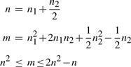
Let G be a genome with n genes, n₁ adjacencies, and n₂ telomeres. If m is the number of the different possible DCJ operations on G, we can write

PROOF. —

G has n genes and thus 2n tails and heads of genes; as the tail or the head of any gene appears in exactly one adjacency or telomere, we have

(1)

Now consider the four cases of DCJ operations:

1. There are ways to select two adjacencies and two possible DCJ operations for each such choice, for a total of operations.

2. There are n₁×n₂ ways to select one adjacency and one telomere and two possible DCJ operations for each combination, for a total of n₁×n₂×2 operations.

3. There are ways to select two telomeres and one possible DCJ operation for each such choice, for a total of operations.

4. There are n₁ different ways to select one adjacency and one possible DCJ operation for each such choice, for a total of n₁ operations.

Thus the total number of possible DCJ operations is

Combining this result with (1), we get

(2)

Now we also have 0≤n₂≤2n, and so we can write

 ▪

3 METHODS

3.1 An overview of our technique for estimating the true evolutionary distance

The problem of estimating the true evolutionary distance under DCJ model is defined as follows:

Input: The original genome G and the final genome G^F, two genomes on the same n genes represented as adjacencies and telomeres.

Output: An estimate of the actual number of DCJ operations that took place in the evolutionary history to transform G into G^F.

Based on the original genome G, for any genome G^* (of same gene content as G), we can divide the adjacencies and telomeres of G^* into four sets , , and , where is the set of adjacencies of G^* that also appear in G, is the set of telomeres of G^* that also appear in G, is the set of adjacencies of G^* that do not appear in G and is the set of telomeres of G^* that do not appear in G. Then we can calculate a vector 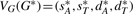to represent the genome G^* based on G, where , , and are the cardinalities of the sets , , and , respectively. (V_G may be viewed as producing a fingerprint of G^*.) Obviously, we have

(3)

Let G^k be the genome obtained from G=G⁰ by applying k randomly selected DCJ operations—under our model, the (i+1)th DCJ operation is selected from a uniform distribution of all possible DCJ operations on the current genome Gⁱ. We can compute the vector to represent the genome G^k with respect to G. In the next section, we will show that, given G, we can also produce the estimate 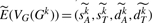for the expected vector 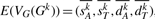, for any integer k>0. We use to approximate the expected number of adjacencies present in both G and G^k. Our approach for estimating the true evolutionary distance is then to return the integer k that minimizes the difference .

3.2 Estimation of the expected vector after some number of random DCJ operations

We show how to estimate the expected vector 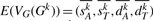under our DCJ model for any integer k>0. Let G and G^k be as defined above; the vector for G⁰ =G is clearly just V_G(G⁰)=(n₁,n₂,0,0). We first show how to compute E(V_G(G¹)).

THEOREM 2. —

Let m be the number of possible DCJ operations applicable to G. We have , where

PROOF. —

Write and consider the four cases for DCJ operations.

1. When we select two adjacencies out of , the number of possible DCJ operations is . Neither of the resulting adjacencies will be in G, so that every such operation reduces by 2 and increase by 2.

2. When we select one adjacency out of and one telomere out of , the number of possible DCJ operations is . Neither of the resulting adjacency nor telomere will be in G, so that every such operation reduces both and by 1 and increases both and by 1.

3. When we select two telomeres out of , the number of possible DCJ operations is . The resulting adjacency will not be in G, so that every such operation will reduce by 2 and increase by 1.

4. When we select one adjacency out of , the number of possible DCJ operations is . Neither of the resulting telomeres will be in G, so that every such operation reduces by 1 and increases by 2.

Adding up the four cases and normalizing by the total m, we get

 ▪

Let G^k be a genome obtained from G by applying k randomly selected DCJ operations and let Ġ^k+1 be the genome obtained from the genome G^k by applying one more randomly selected DCJ operation. We show how to calculate the expected value of V_G(Ġ^k+1) given G^k and G.

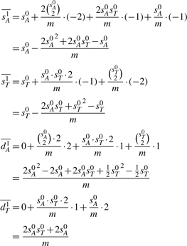
THEOREM 3. —

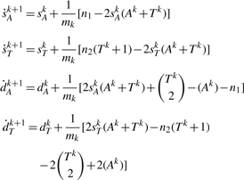
Let and let m_k be the number of possible DCJ operations on G^k. For conciseness, write (the number of adjacencies in G^k) and (the number of telomeres in G^k). Then we can write

where we have

(4)

(5)

(6)

PROOF. —

From Theorem 1, we have

There are adjacencies in G that do not appear in G^k and they must fall into one the following three cases:

1. n_AA pairs with members in two different adjacencies in .

2. n_TT pairs with members in two telomeres of .

3. n_AT pairs with one member in and the other in .

There also are telomeres in G that do not appear in G^k and so must be members of .

Now we complete the proof by running through the possible cases. From the proof for Theorem 2, we have already covered four cases where adjacencies and telomeres were selected only from and . The remaining eight cases cover selections from and as well. In the last five of these eight cases, the outcome of a particular operation in terms of adjacency and telomere counts is not fixed, but the total count over all possible operations can still be computed; we use the expression ‘recover’ (an adjacency or a telomere) to indicate a case in which the count increases.

1. When we select one adjacency out of and another out of , the number of possible DCJ operations is . Neither resulting adjacency will be in G, so that every such operation reduces by 1 and increases by 1.

2. When we select one adjacency out of and one telomere out of , the number of possible DCJ operations is . Neither the resulting adjacency nor telomere will be in G, so that every such operation reduces by 1 and increases by 1.

3. When we select one telomere out of and one telomere out of , the number of possible DCJ operations is . Neither the resulting adjacency nor telomere will be in G, so that every such operation reduces and by 1 and increases by 1.

4. When we select one telomere out of and one adjacency out of , the number of possible DCJ operations is . The resulting adjacency will not be in G, while the resulting telomere can be in G or not. There are ways to recover one telomere out of telomeres in G that do not appear in G^k.

5. When we select two adjacencies out of D_A, the number of possible DCJ operations is . The two resulting adjacencies can be in G or not. There are n_AA ways to recover one adjacency out of adjacencies in G that do not appear in G^k.

6. When we select one adjacency out of and one telomere out of , the number of possible DCJ operations is . The resulting adjacency and telomere can be in G or not. There are ways to recover one telomere out of telomeres in G that do not appear in G^k and n_AT ways to recover one adjacency out of adjacencies in G that do not appear in G^k.

7. When we select one adjacency out of , the number of possible DCJ operations is . The two resulting telomeres can be in G or not and there are ways to recover one telomere out of telomeres in G that do not appear in G^k.

8. When we select two telomeres out of , the number of possible DCJ operations is . The resulting adjacency can be in G or not and there are n_TT ways to recover one adjacency out of adjacencies in G that do not appear in G^k.

Adding up the 12 cases and normalizing by the total m_k, we get

 ▪

Given G⁰, we estimate E(V_G(G^k)) for k>0 by iterating k times the matching formula in Theorem 3, and every time we identify E(V_G(G^k−1)) with the actual vector V_G(G^k−1).

COROLLARY 1. —

Let G be one genome on n genes, the estimated vector for all integers i (0≤i≤k) can be computed in O(k) time.

3.3 Asymptotic behavior of our estimation

We can use our results to derive the ‘stable’ structure of a genome under the random DCJ model—the structure reached after sufficiently many events.

COROLLARY 2. —

Let G have n (n≥2) genes; then the estimated vector and the estimated number of possible DCJ operation for genome G^k satisfy

(7)

(8)

The fairly technical proof is attached in Appendix; the approach is to define , with , and to consider separately the cases where ɛ₀ is positive and negative, showing in each case that ɛ_k keeps the sign of ɛ₀ and that the limit of ɛ_k as k grows is zero.

COROLLARY 3. —

If the estimated vector is and if we have n≥2, then we can write

PROOF. —

We first calculate . From formula (4) in Theorem 3 and formula (3), we have

(9)

Combining formulae (7), (8) and (9), together with , we get

Similarly, we can calculate the limits for , and . ▪

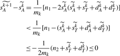
COROLLARY 4. —

If we have n₁≥1, then our estimated value decreases monotonically with k until .

PROOF. —

From the assumption n₁≥1, we have . Now it is enough to show that, for any integer k, if we have , then we get . If we have , then, from formula (4) in Theorem 3, we have,

 ▪

These three corollaries paint a picture of the long-term consequences on genomic structure of random DCJ events; in particular, they predict that the number of linear chromosomes (half of the number of telomeres) converges to and also, intuitively enough, that the number of shared adjacencies, , goes down to (effectively) zero. The prediction of the asymptotic number of linear chromosomes illustrates the limitations of the method: for humans, for instance, using a figure of 25000 genes, we get an asymptotic number of 112 chromosomes—and it is to be doubted whether, even with a billion more years of evolution, the human genome would ever feature these many chromosomes. Another example is that of bacteria, which usually have a single circular chromosome, not the 22–50 linear chromosomes that would go with 1000–5000 genes. Clearly, the uniform model is too simple and constraints exist in organismal genomes that strongly dampen chromosomal fission. At present, however, there are too many ways in which to impose such constraints within the DCJ model and not enough data to decide which way is best.

4 EXPERIMENTS

We now present experimental results on the accuracy of our estimation of the expected vector after a given number of random DCJ operations and on the quality of our estimator for the true evolutionary distance (in terms of the actual number of DCJ operations). Our experiments all start with an original genome, G, with some chosen number of linear and circular chromosomes of various sizes; this genome is subjected to a prescribed number k of DCJ operations chosen uniformly at random to obtain a final genome G^k. We vary k from one to six times the number of genes—very large values in evolutionary terms. For each choice of parameters, we generate 10 000 runs to obtain a tight estimate of variance. We compute the vector representations for all intermediate genomes and then use our method to estimate the evolutionary distance. We ran tests on a large variety of initial genomes, some designed to resemble actual organismal genomes, some entirely unrealistic to test extreme cases. Due to space limitations, we present results on just three initial genomes, all meant to resemble real organismal genomes: (a) 25 000 genes and 25 linear chromosomes; (b) 10 000 genes and 5 linear chromosomes and (c) 1000 genes and 1 circular chromosome—the first two examples match metazoan genomes, the last matches a small bacterial genome.

4.1 Accuracy of the expected vector after k-random DCJ operations

We study the behavior of our estimation by comparing its prediction to the sample mean for E(V_G(G^k)), as computed from our 10 000 trials. We include an additional, extreme, genome with 5000 genes and 2500 linear chromosomes to show that our technique works across a very broad range of parameters. In all of our experiments, we find that is extremely close to the sample mean for E(V_G(G^k)): the maximum absolute error of corresponding values between our estimation and the sample mean is always <0.8. Figure 2 shows the four values in the vector as a function of the actual number of DCJ operations for genome (a) (the curves for genomes (a), (b) and (c) are similar) and for the ‘extreme’ genome (where the curves are better differentiated). The figure does not distinguish our estimation and the sample mean for E(V_G(G^k)), because the difference is too small with respect to the actual value. We also compute the mean absolute difference for s_A, s_T, d_A, and d_T between our estimation and each experimental vector V_G(G^k) in every single run for genomes (a), (b) and (c) and show the results in Figure 3. The sum of absolute difference of entries in the vector on the larger genomes never exceeds 0.5% (as a percentage of the sum of entries in the vector) and is typically well below 0.25%; even on the smaller genome, the difference does not exceed 2% and is typically below 1%.

Fig. 2.

The four vector values as a function of the actual number of DCJ operations.

Fig. 3.

The mean absolute difference for s_A, s_T, d_A and d_T between our estimation and each experimental vector V_G(G^k) as a function of the actual number of DCJ operations.

4.2 Accuracy of the estimation of the actual number of DCJ operations

We want to study the threshold of saturation of our estimator in addition to its accuracy; in order to do that, we create simulations with controlled numbers of DCJ operations and set up a threshold for correction in the estimation procedure. Specifically, we choose a number between 1 and some upper bound B as the actual number of DCJ operations; B is chosen to be the smallest integer k that makes the expected value  <2, a point at which there are almost no shared adjacencies left (from Corollary 4). For genomes (a), (b) and (c), the corresponding upper bounds are 121 621, 44 047 and 3253, respectively. From Corollaries 3 and 4, and the fact n₁≤n, we have 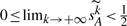. Thus we use the smallest integer r that causes the expected value to become smaller than 1/2 as an upper limit on the maximum number of DCJ operations in the evolutionary history. Finally, if we have , we set k (the value normally chosen to minimize ) to this upper limit r. For genomes (a), (b) and (c), r has values 211 442, 81 329 and 6398, respectively.

Figure 4 shows the mean and SD for the actual number of DCJ operations estimated by the edit DCJ distance and by our approach. These figures indicate that, as expected, the edit DCJ distance underestimates, often severely, the actual number of events. In contrast, our approach provides highly accurate estimates, with very small variance.

Fig. 4.

Mean and SD plots for the actual number of DCJ operations (y-axis) versus the edit DCJ distance and our estimator (x-axis). The datasets are divided into 60 bins according to their x-coordinate values.

We also study the mean absolute difference between the actual number of DCJ operations and our estimator for genomes (a), (b) and (c). The results are shown in Table 1. The estimates are highly accurate (even for small genomes) up to surprisingly large numbers of events. Rearrangements events fall under the category of ‘rare genomic events’ [in the terminology of Rokas and Holland (2000)], yet our estimator works well even for what would be considered common events.

Table 1.

The mean absolute difference between actual number of DCJ operations and our estimation

No. of genes	Actual number of DCJ operations
	No. of genes ×1	No. of genes ×2	No. of genes ×3
25 000	131.0 (0.5%)	447.5 (0.9%)	1280.2 (1.7%)
10 000	83.9 (0.8%)	282.0 (1.4%)	819.4 (2.7%)
1000	27.2 (2.7%)	93.6 (4.7%)	441.8 (14.7%)

5 DISCUSSION AND CONCLUSIONS

From Sections 4.1 and 4.2, our estimation achieves very high accuracy, especially for larger (metazoan) genomes. From Figure 4, our approach postpones the threshold of saturation (viewed as a number of DCJ operations) from well under the number of genes to at least three times the number of genes for all three example genomes. This large gain in accuracy should translate into much better phylogenetic reconstructions as well as more accurate genomic alignments.

Moreover, Corollaries 2 and 3 make specific predictions about the structure of evolved genomes on n genes after many steps: namely, that all should have approximately telomeres, that is linear chromosomes, and that shared adjacencies with other highly evolved genomes should be nearly absent. While the second prediction is intuitively reasonable, it is in fact rarely satisfied in actual organisms, especially for small genomes (such as prokaryotic genomes), where conservation pressures are very high and specific structures such as operons survive across broad ranges of evolutionary divergence. The first prediction is, as noted earlier, nearly always overstated: clearly, biological constraints prevent chromosomal fission to be as commonplace as the uniform DCJ mechanism would appear to suggest.

These predictions rely on the two main assumptions made in this work: no gene duplication or loss; and uniform distribution of DCJ operations. Both are clearly unrealistic, so our ability to gauge their effect on model predictions is crucial to future model refinements.

For instance, in their original paper, Yancopoulos et al. (2005) required that a chromosomal fission that creates a new small circular chromosome be immediately followed by a chromosomal fusion that re-absorbs this small circular chromosome, thereby causing a block exchange within the original chromosome and treating the extra circular chromosome as a transient artifact. Since circular chromosomes do not arise in organisms with a number of linear chromosomes, a similar constraint would strongly reduce the incidence of fission. A similar type of constraint could be used for prokaryotic genomes, which normally consist of a single circular chromosome. Using just such a constraint, Kothari and Moret (2007) found that the DCJ edit distance closely reflected both inversion and transposition operations. Evidence that paracentric rearrangements are more common than pericentric ones, at least in two Drosophila species (York et al., 2007), and that short inversions are more common than long ones, in some prokaryotes and in the aforementioned Drosophila (Lefebvre et al., 2003; York et al., 2007), can also be reflected into additional constraints on the DCJ model. Any additional constraint naturally creates complications, but we expect that at least a few natural constraints can be handled within the framework described here.

Some significant advances have been made by our group for handling duplications and losses in an inversion context (see, e.g. Marron et al., 2004; Swenson et al., 2005; Tang et al., 2004); since duplications and losses are handled in that work mostly through the greedy approach of using rearrangements to place together genes that can then be gained or lost in a single operation, moving this work to a DCJ context appears uncomplicated. This combination could then yield the first reliable estimate of genomic pairwise distances for complex metazoan genomes based on rearrangements and duplication/loss mechanisms.

Finally, since the DCJ operation regroups all rearrangements studied to date, and since our results point to one way in which the behavior of this model can be studied for various constraints (such as where the cuts can be made), our results may shed light on the vexing issue of what constitutes a significant syntenic block in comparative genomics—an issue that has seen a lot of discussion over the last few years. [Sinha and Meller (2008) give a review of these discussions and some proposals, while Chaisson et al. (2006) give evidence that rearrangements occur at multiple scales.]

Conflict of Interest: none declared.

APPENDIX

Proof of Corollary 2:

PROOF. —

We have , , and , and so can write

with

We now consider two cases: (i) and (ii) 0 ≤ ɛ₀ ≤. In each case, we prove by induction on k the following result for :

(A1)

Case (i) We have and, by inductive hypothesis, . We now bound the range for ɛ_i+1 .

From formulae (5) and (6) in Theorem 3 as well as formula (3), we have

Replacing and by and , we get

(A2)

From formula (2), we have

(A3)

From Formula (A3) and our inductive hypothesis, and using n≥2, we get

(A4)

Then from formulae (A2) and (A4), we can write

and from the inductive assumption and by using n≥2, we can verify that ɛ_i+1 satisfies

Since we have , then, by induction, we have, for any integer k,

and thus, with n≥2,

Case (ii) We have and, by inductive hypothesis, . We now bound the range for ɛ_i+1 .

From formula (A3) and the inductive hypothesis, and using n≥2, we can write

(A5)

Now using formulae (A2) and (A5), we get

and from the inductive hypothesis and using n≥2, we can verify that ɛ_i+1 satisfies

Since we have , then, by induction, we have, for any integer k,

and thus, with n≥2,

Putting it all together, we have

Moreover, from formulae (A1) and (A3), we can write

 ▪

REFERENCES

- Bader D, et al. A fast linear-time algorithm for inversion distance with an experimental comparison. J. Comput. Biol. 2001;8:483–491. doi: 10.1089/106652701753216503. [DOI] [PubMed] [Google Scholar]
- Bergeron A, et al. Vol. 4175in Lecture Notes in Computer Science. Springer Verlag; 2006. A unifying view of genome rearrangements. In; pp. 163–173. [Google Scholar]
- Chaisson M, et al. Microinversions in mammalian evolution. Proc. Natl Acad. Sci, USA. 2006;103:19824–19829. doi: 10.1073/pnas.0603984103. [DOI] [PMC free article] [PubMed] [Google Scholar]
- Durrett R, et al. Bayesian estimation of the genomic distance. Genetics. 2004;166:621–629. doi: 10.1534/genetics.166.1.621. [DOI] [PMC free article] [PubMed] [Google Scholar]
- Hannenhalli S, Pevzner P. ACM Press; Transforming cabbage into turnip (polynomial algorithm for sorting signed permutations by reversals). In; pp. 178–189. Proceedings of the 27th Annual ACM Symposium on the Theory of Computing (STOC'95) [Google Scholar]
- Hannenhalli S, Pevzner P. IEEE Press; 1995b. Transforming mice into men (polynomial algorithm for genomic distance problems). In; pp. 581–592. Proceedings of the 36th Annual IEEE Symposium on Foundations of Computer Science (FOCS'95) [Google Scholar]
- Kothari M, Moret B. IEEE Press; 2007. An experimental evaluation of inversion- and transposition-based genomic distances. In; pp. 151–158. Proceedings of the 3rd IEEE Symposium on Computational Intelligence in Bioinformatics and Computational Biology (CIBCB'07) [Google Scholar]
- Lefebvre J-F, et al. Detection and validation of single gene inversions. In. Bioinformatics. 2003;19:i190–i196. doi: 10.1093/bioinformatics/btg1025. Proceedings of the 11th International Conference on Intelligent Systems for Molecular Biology (ISMB'03) [DOI] [PubMed] [Google Scholar]
- Marron M, et al. Genomic distances under deletions and insertions. Theor. Comput. Sci. 2004;325:347–360. [Google Scholar]
- Moret B, et al. New approaches for reconstructing phylogenies from gene-order data. In. Bioinformatics. 2001;17:S165–S173. doi: 10.1093/bioinformatics/17.suppl_1.s165. Proceedings of the 9th International Conference on Intelligent Systems for Molecular Biology (ISMB'01) [DOI] [PubMed] [Google Scholar]
- Moret B, et al. Steps toward accurate reconstructions of phylogenies from gene-order data. J. Comput. Syst. Sci. 2002;65:508–525. [Google Scholar]
- Moret B, et al. Reconstructing phylogenies from gene-content and gene-order data. In. In: Gascuel O, editor. Mathematics of Evolution and Phylogeny. Oxford: Oxford University Press; 2005. pp. 321–352. [Google Scholar]
- Rokas A, Holland P. Rare genomic changes as a tool for phylogenetics. Trends Ecol. Evol. 2000;15:454–459. doi: 10.1016/s0169-5347(00)01967-4. [DOI] [PubMed] [Google Scholar]
- Sankoff D, Blanchette M. Multiple genome rearrangement and breakpoint phylogeny. J. Comput. Biol. 1998;5:55–570. doi: 10.1089/cmb.1998.5.555. [DOI] [PubMed] [Google Scholar]
- Sankoff D, Blanchette M. ACM Press; 1999. Probability models for genome rearrangement and linear invariants for phylogenetic inference. In; pp. 302–309. Proceedings of the 3rd Annual International Conference on Computational Molecular Biology (RECOMB'99) [Google Scholar]
- Sinha A, Meller J. World Scientific; 2008. Sensitivity analysis for reversal distance and breakpoint reuse in genome rearrangements. In; pp. 37–48. Proceedings of the 13th Pacific Symposium on Biocomputing (PSB'08) [PubMed] [Google Scholar]
- Swenson K, et al. SIAM Press; 2005. Approximating the true evolutionary distance between two genomes. In; pp. 121–129. Proceedings of the 7th SIAM Workshop on Algorithm Engineering & Experiments (ALENEX'05) [Google Scholar]
- Swenson K, et al. Advances in Bioinformatics and Computational Biology. Imperial Press; 2008. Phylogenetic reconstruction from complete gene orders of whole genomes. Vol. 6 in; pp. 241–250. [Google Scholar]
- Swofford D, et al. Phylogenetic inference. In. In: Hillis D, et al., editors. Molecular Systematics. Sunderland, MA: Sinauer Assoc; 1996. pp. 407–514. [Google Scholar]
- Tang J, et al. IEEE Press; 2004. Phylogenetic reconstruction from arbitrary gene-order data. In; pp. 592–599. Proceedings of the 4th IEEE Symposium on Bioinformatics and Bioengineering (BIBE'04) [Google Scholar]
- Wang L-S. ACM Press; 2001. Exact-IEBP: a new technique for estimating evolutionary distances between whole genomes. In; pp. 637–646. Proceedings of the 33rd Annual ACM Symposium on Theory of Computing (STOC'01) [Google Scholar]
- Wang L-S, Warnow T. Lecture Notes in Computer Science. Springer Verlag; 2001. Estimating true evolutionary distances between genomes. Vol. 2149 in; pp. 176–190. [Google Scholar]
- Yancopoulos S, et al. Efficient sorting of genomic permutations by translocation, inversion and block interchange. Bioinformatics. 2005;21:3340–3346. doi: 10.1093/bioinformatics/bti535. [DOI] [PubMed] [Google Scholar]
- York T, et al. Dependence of paracentric inversion rate on tract length. Bioinformatics. 2007;8 doi: 10.1186/1471-2105-8-115. (online publication) [DOI] [PMC free article] [PubMed] [Google Scholar]