Nucleosome positioning from tiling microarray data

Abstract

Motivation: The packaging of DNA around nucleosomes in eukaryotic cells plays a crucial role in regulation of gene expression, and other DNA-related processes. To better understand the regulatory role of nucleosomes, it is important to pinpoint their position in a high (5–10 bp) resolution. Toward this end, several recent works used dense tiling arrays to map nucleosomes in a high-throughput manner. These data were then parsed and hand-curated, and the positions of nucleosomes were assessed.

Results: In this manuscript, we present a fully automated algorithm to analyze such data and predict the exact location of nucleosomes. We introduce a method, based on a probabilistic graphical model, to increase the resolution of our predictions even beyond that of the microarray used. We show how to build such a model and how to compile it into a simple Hidden Markov Model, allowing for a fast and accurate inference of nucleosome positions.

We applied our model to nucleosomal data from mid-log yeast cells reported by Yuan et al. and compared our predictions to those of the original paper; to a more recent method that uses five times denser tiling arrays as explained by Lee et al.; and to a curated set of literature-based nucleosome positions. Our results suggest that by applying our algorithm to the same data used by Yuan et al. our fully automated model traced 13% more nucleosomes, and increased the overall accuracy by about 20%. We believe that such an improvement opens the way for a better understanding of the regulatory mechanisms controlling gene expression, and how they are encoded in the DNA.

Contact: nir@cs.huji.ac.il

1 INTRODUCTION

In eukaryotic cells the DNA is packed within the nucleus where it is wrapped around protein complexes called nucleosomes, such that each nucleosome is surrounded by roughly 147 DNA bases (Luger et al., 1997). This packaging facilitates the storage and organization of the long eukaryotic chromosomes. It also plays a crucial role in regulation of DNA-related processes by modulating the accessibility of DNA to regulatory proteins. Specifically, linker DNA regions between nucleosomes are exposed to binding of transcription factors that can thereby affect the expression of nearby genes (Buck and Lieb 2006). As these regulatory DNA binding sites are typically short (5–20 bp), knowing the exact location of nucleosomes along the DNA is crucial for understanding the transcriptional blueprints embedded in the DNA (e.g. Narlikar et al., 2007).

Several recent works measured nucleosome positions along the DNA in a high-throughput manner. This involves extracting DNA occupied by nucleosomes either by using chromatin immunoprecipitation (ChIP) assays (Pokholok et al., 2005), or digestion of linker regions by micrococcal nuclease (MNase) (Albert et al., 2007; Lee et al., 2007; Raisner et al., 2005; Yuan et al., 2005). These nucleosome occupied regions are then mapped either by hybridization to tiling DNA microarrays (Lee et al., 2007; Pokholok et al., 2005; Raisner et al., 2005; Yuan et al., 2005), or by high throughput DNA sequencing (Albert et al., 2007; Schones et al., 2008; Shivaswamy et al., 2008). Additional works identified positioning signals embedded in the DNA sequence, and used them to estimate preferred nucleosome positions (Ioshikhes et al., 1996, 2006; Peckham et al., 2007; Segal et al., 2006; Yuan and Liu, 2008).

In this work, we present a fully automated computational method to identify nucleosome positions based on the raw output of microarray measurements of MNase-based assay (e.g. Yuan et al., 2005). Our emphasis is on improving the resolution of these nucleosome calls beyond that of the microarray platform used. We do so using a probabilistic graphical model that describes how probe values depend on the exact nucleosome positions. We applied our model to nucleosomal data from mid-log yeast cells reported by Yuan et al. (2005), and compared our predictions of nucleosome calls to the original study, to those of a more recent high-throughput method that uses higher resolution tiling arrays (Lee et al., 2007), and to a curation of literature-based positions (Segal et al., 2006). Our results suggest that by applying our algorithm to the same data of Yuan et al. we were able to trace more nucleosomes, and increase the overall accuracy.

2 PROBABILISTIC MODEL FOR NUCLEOSOME CALLS

2.1 Experimental data

To estimate the exact position of nucleosomes along the DNA in yeast cells, we analyzed the tiling microarray data of Yuan et al. (2005). In this work, MNase assay was used to digest linker DNA regions resulting in mononucleosomal DNA fragments of length ∼150 bp. These nucleosome fragments were then labeled with fluorescent dye and hybridized to microarrays against a total genomic DNA reference. Yuan et al.'s microarrays were designed with overlapping 50 bp long probes tiled every 20 bp across the entire Saccharomyces cerevisiae Chromosome 3 and additional regions of interest, such as gene promoters, covering about 4% of the yeast genome.

The interpretation of these arrays is that probes corresponding to stretches of DNA protected by nucleosomes will be enriched in comparison to the genomic reference. On the other hand probes that correspond to linker regions will be depleted. Thus, by examining the log ratio of signals between the two channels (nucleosome versus genomic), we can identify nucleosome protected regions (Fig. 1).

Fig. 1.

Raw data from Yuan et al. shown on 600 bp of Chromosome 3 (79 000–79 600), mapped onto probe locations. Top: raw log ratio (black line) of nucleosome occupied DNA against genomic DNA. Bottom: design of tiling array, where each rectangle denotes the location of a probe and the vertical dotted line maps it to its measured value. These probe locations were marked with nucleosomal occupancy based on Yuan et al.'s predictions (thick grey bars), where each probe is assigned either to be nucleosome occupied (grey) or not (black).

Although the general shape of these data is well coordinated with nucleosomes, naive prediction of their positions, e.g. using a fixed threshold over the log ratios is difficult. Among other reasons, this is due to global trends in the hybridization baseline value, varying along the genome.

2.2 Model of Yuan et al.

To analyze these data, and infer the position of nucleosomes, Yuan et al. developed a Hidden Markov model (HMM). In their model, each probe i is mapped onto two random variables: N_i, a hidden variable that denotes the relative location of this probe within a nucleosome (or equals zero if the probe resides within a linker DNA), and P_i, the observed value of this probe (Fig. 2a). As each nucleosome covers about 147 bp, and since every pair of consecutive probes overlap in 30 bp, each nucleosome spans over 7–8 probes (Fig. 1). Their HMM allowed each N_i to take one of eight internal states, plus an additional ‘linker’ state. The transition matrix Pr(N_i+1|N_i) allows non-zero transitions only from the linker to the first nucleosome state, and from each relative position to its subsequent state (Fig. 2b). This basic model was further corrected to allow for longer or shorter nucleosomes that often appear in the data. This was done by allowing transitions from states six and seven to the linker state. In addition, they added a second set of nine internal states, as represented by the outer circle in Figure 2b, to represent ‘fuzzy’ nucleosomes that are not well localized. This nucleosomal model has only five transition parameters. These include the probabilities of entering a nucleosome, and those of returning to the ‘linker’ state.

Fig. 2.

(a) HMM by Yuan et al. Each hidden N_i variable represents the relative position of probe i within a nucleosome, and can take each of the states shown in the diagram (b). Each P_i variable represents the observed hybridization ratio of probe i. (b) The state diagram of the HMM. The inner circle represents the well-localized nucleosomes, while the outer circle represents the ‘fuzzy’ ones. (c) To avoid over-fitting, the emission-probability estimation is independent of both the relative position in a nucleosome and its type. Thus there are only two conditional distributions modeling the probability for the observed hybridization ratio given a nucleosomal and a linker probe shown in solid and dashed lines, respectively.

Given an assignment to the N_i variables, the emission probabilities of the observed states P_i were modeled as coming from one of two Gaussian distributions, shown in Figure 2c. This assumes that each population of probes (originating from nucleosomal, or linker DNA) displays a different distribution of values.

An assignment to the N_i variables that maximizes the posterior probability given the measured probe values, can be found by performing inference in this HMM. This allows to call nucleosomes from the data. Yuan et al. noted that there are global trends in the data that change the baseline values of stretches of probes. This causes the HMM trained on one part of the data to perform poorly on regions with a different baseline. To account for the local baseline, they applied their HMM to overlapping segments of 40 probes, and for each segment, they learned the parameters of the model separately. They also used an additional method to identify very low-ratio nucleosomes, which were not originally found by the HMM. Finally, their predictions underwent a hand-curation phase to correct what they perceived to be missing or wrong nucleosome calls.

2.3 Our model

The approach of Yuan et al. suffers from several drawbacks. These involve two (related) issues. First, since their model is defined over the measured probes, it is inherently limited to the array's 20 bp resolution. This binary assignment, where probes are either inside or outside of nucleosomes might be too simplified, as partially hybridized probes (e.g. at nucleosome boundaries) usually result in intermediate value (see examples in Figure 1). Second, their HMM model is sensitive to global trends, and thus requires a combination of solutions, on top of the model (e.g. running on small segments, hand curation).

We now describe a model that deals with both these issues within the probabilistic model. This will allow us to automate the analysis of such data and extract more precise nucleosome calls.

Our model is similar in nature to the HMM of Yuan et al. in that there is a chain of hidden variables that denote the nucleosomal state. However, unlike their model, we decouple the representation of nucleosomes from probe locations. Thus, the hidden layer represents nucleosome locations along the genome, and captures constraints on these locations—nucleosomes do not overlap and have minimal-linker region between them. To do so, we introduce a new type of state variables S_j, each representing the status of a 10 bp window. This status can be either ‘linker’ or a location within the nucleosome. More precisely, the S_j variables can take 15 states (to span the length of a nucleosome). In our model, the value of S_j+1 depends on the value of S_j according to the transition diagram shown in Figure 3a. To allow for slightly shorter nucleosomes, we introduce transitions from state seven that can lead to nucleosomes in the range of 120–140 bp.

Fig. 3.

(a) Our state diagram for the state variables S_j. (b) Graphical model: the hidden S_j variables report the position of a genomic locus with regard to an overlapping nucleosome (in 10 bp resolution), or zero in case of a linker DNA region. The hidden C_i variables hold the maximal coverage of a probe by a nucleosome, as reported by the relevant S_j's. The hidden L_i variables are the inferred-occupancy levels for each probe, and the P_i variables are the probes’ measured values. (c) The compiled meta-HMM: the states of X_i's denote the combination of S_j,L_i variables connected to probe i. P_i are as in (b).

The next question is how to relate the status of the nucleosomes with the observed probe values. Each probe is 50 bp long and spans five consecutive S_j variables. If all five variables are nucleosome occupied (states between 1 and 14), then DNA position matching the probe is expected to be fully protected from MNase digestion and the probe will have a high nucleosome to control ratio. On the other hand, if all five variables are in a linker state, then the probe sequence is not protected, and the probe will have a low nucleosome to control ratio. On nucleosome boundaries only part of the nucleosome sequence is protected, and we expect intermediate signals. Indeed, this is exactly what we see in the raw data (e.g. Figure 1). When combining such boundary probes together with mid-nucleosome probes, as done by Yuan et al. we get a wide distribution of probe values, which reduces the information the model can extract from these values. If instead we assume a separate distribution for boundary probes, we can learn much tighter distributions and extract more information from the observed values.

To capture these effects, we introduce an additional layer of variables, one per probe, which represent the size of the largest continuous fraction of the probe that is protected by a nucleosome. For probe i we denote by the max-coverage variable C_i, that can take six values: 0,20,…, 100%. These values are a deterministic function based on the values of the corresponding S_j's (Fig. 3b). The observed hybridization level of the probe will depend on the associated max-coverage variable.

As we stated earlier, another issue we have to deal with is changes in the regional-baseline value. These changes can occur for several consecutive nucleosomes or at the level of a single nucleosome. Thus, we want to model the relevant baseline level variable L_i that is relevant for each probe. For simplicity, we discretize baseline levels into four possible values. To capture the regional effect of the baseline we require that the values of the L_i variables remain fixed within nucleosomes. Specifically, each L_i+1 depends on both L_i and the state variables S_j in the intermediate region. If these are within a nucleosome, then L_i=L_i−1, otherwise, L_i is chosen from a prior over occupancy levels (Fig. 3b).

The final component in the model is the probability of observing different values at each probe. As in Yuan et al.'s model, for each probe i we add the observed hybridization ratio P_i. Given the assignment of the occupancy level and the coverage for this probe, the probability P(P_i∣C_i,L_i) is a Gaussian distribution, whose parameters are defined by the parent variables (C_i and L_i). The final model is shown in Figure 3b. The ability to learn different parameters for a combination of levels and coverage is one of the strengths of our model. When learning from the raw data of Yuan et al. (see below for details), we get a distinct range of values for each of these combinations as seen in Figure 4. In particular, note that the variance of full coverage (100%) is much smaller in our model. This is due to the distinction between full coverage and partial coverage. Also note that the value of full coverage in a ‘medium’ baseline level nucleosome corresponds to the value of partial coverage in a ‘high’ baseline. This demonstrates why shifts in the baseline interfere with inference in Yuan et al.'s model. Our model forces all the probes in a nucleosome to be in the same baseline, and thus the signal it enforces is one where the mid-nucleosome probes are higher than the boundary ones.

Fig. 4.

A representation of the conditional Gaussians learned in our model for high and medium baseline in linker (0%), boundary (60%) and mid-nucleosomal (100%) probes, and their comparison to the Gaussians in Yuan et al.'s model. For each case we plot the mean of the Gaussian (vertical bar) and the range of ±1 SD.

2.4 Learning the model

To tune the model we need to learn parameters. These parameters include the θ and ψ parameters that govern the state distribution of S_j (Fig. 3a), the priors on baseline levels, and the mean and variance of the conditional Gaussians that govern the probe values (given the baseline and coverage variables).

We start by noting that if we had an assignment of nucleosome positions and the baseline level of each one, learning is straight-forward. In such a situation, we can learn these parameters using standard maximum likelihood estimation. This involves collecting the following statistics: the average length of linker DNA segments (governing the θ parameter), the distribution of nucleosome lengths (governing the ϕ parameters), the number of nucleosomes in each baseline (governing the baseline prior), and the mean and variance of observed hybridization values for different classes of probes (governing the probe-emission probabilities).

The question is how to build an estimate of nucleosome positions to bootstrap the learning process. Such an assignment can be derived by a piecewise linear spline model, capturing the typical trace of a nucleosome in the raw data. Alternatively, we can initialize our learning process with the nucleosome calls of Yuan et al. Our analysis shows that both initializations, although different, lead to fairly similar parameters (data not shown). To initialize the level variables (L_i), we divide the nucleosomes into three equally sized groups (covering 90% of the nucleosomes), and an additional group of low-occupancy nucleosomes. These assignments were used to estimate the emission probability of each level, using maximum-likelihood estimation. The parameter estimations can be further improved by applying a standard iteration Expectation–Maximization procedure (Dempster et al., 1977). However, in our experiment such iterations lead only to minor changes in the parameter values, and thus were not applied eventually.

2.5 Model compilation

The model, as presented in Figure 3b, is densely connected due to overlapping probes introducing loops between the S and the C variables. This makes standard exact inference methods, such as variable elimination or clique tree propagation (Pearl 1988), extremely time consuming. One possible solution in such models is to collapse a set of densely connected variables into one meta-variable. In general, this is usually associated with an exponential blowup in the cardinality of these meta-variables. This is especially problematic in our model, where the cardinality of the random variables is large to begin with (e.g. 15 possible assignments for the state variables S_j).

We notice, however, that due to the deterministic nature of our transition matrices, we can create such meta-variables without the associated complexity. This gives us the leverage of both having a very detailed model, while enabling exact inference.

We developed an automated procedure to compile a graphical model such as the one in Figure 3b into a simpler HMM (shown in Figure 3c). The key observation here is that if we look at two consecutive probes spanning over 70 bp, they share the S_j's in the middle 30 bp and differ only in the 20 bp flanking regions. Now we can consider two meta-variables, each containing all the variables affecting the hybridization ratio of its corresponding probe. The transition between these two meta-variables might be naively represented by a huge matrix containing all possible assignments for each meta-variable. Fortunately, this matrix is extremely sparse, since the two meta-variables need to agree on all the overlapping variables and also due to the deterministic nature of the S_j transition matrix. We now formalize these ideas, and show how we can use them to get an efficient representation of our detailed model with a much simpler meta-HMM.

First, we define the new variable X_i whose state is the cross product of all the variables affecting the hybridization ratio of probe i. These variables include the five S_j variables connected to C_i, and L_i. Thus, the value of X_i is in the space [0−14] × [0−14] × [0−14] × [0−14] × [0−14] × [0−3]. The cardinality of such a meta-variable is larger than 3 million possible assignments.

In the next stage we eliminate states that are impossible due to the conditional probability of variables agglomerated within X_i. For example, if S₁₀=1 then we should consider only assignments to X₁ where S₂₀=2,S₃₀=3 and so on. Generally speaking, since our original transition matrix over the S_j variables is very sparse, many assignments to X_i are unattainable, which results in a massive reduction in the state space of X_i.

Once we define the set of consistent values of these meta-variables, we can define a transition probability between them. This transition is calculated by computing the conditional probability in the original model. In our case,

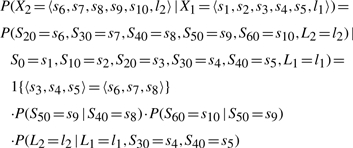Since the state X_i contains all the parents of P_i, the emission probability is exactly as it was in the original model. That is,

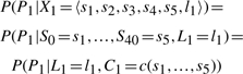where c(s₁,…,s₅) is the deterministic function that maps the five values the S variables to the value of C.

In the final stage, we perform an additional step of simplifying the model. We say that two states of X_i are equivalent if they share the same transition and emission probabilities. Since the transition probability is determined by the last three variables of the state, all states matching 〈·,·,s₃,s₄,s₅,l_i〉 share the same transition probability. So, all states that obey this rule, and share the same emission probability are equivalent (e.g. 〈8,9,10,11,12,l_i〉,〈7,9,10,11,12,l_i〉,〈6,7,10,11,12,l_i〉). It is easy to prove that merging two equivalent states does not change the likelihood of the observations, as this is an instant of state abstraction (Friedman et al., 2000). We thus repeatedly merge equivalent states, updating the transition probability (which can cause other pairs of states to become equivalent), until all states are non-equivalent to each other.

After finishing this process for the model of Figure 3b, we managed to reduce the state space of the meta-variables X_i from about 3 million to only 100 states. Performing exact inference (forward–backward and Viterbi) in this model is straightforward (Rabiner, 1989). Once we have a posterior distribution over the X variables, we can map them to a posterior over the original model variables. Importantly, we have not made any approximations in this compilation process. Thus the results of exact inference in the compiled model are valid also for the detailed one.

3 RESULTS

So far we described an exact and efficient probabilistic graphical model for analyzing measured data of nucleosome positions. We now return to our original task, and predict the location of nucleosomes in a genome-wide manner.

We applied our model to genome-wide data of positions in mid-log yeast cells from Yuan et al. (2005). Given the measured hybridization ratios of all probes, we applied the Viterbi algorithm to find the most probable assignment (MAP) of the S_j variables (Rabiner, 1989). This assignment provides the most likely global arrangement of nucleosomes given the measured data, in 10 bp resolution. Although we will use the MAP assignment from here on to identify nucleosome positions, we can also use the same HMM to calculate the marginal posterior distribution for each S_j. These marginals may be useful in various settings to answer probabilistic queries about the occupancy or position of nucleosomes.

To evaluate the accuracy of our predictions we compared our nucleosome calls to several other sources. First, we consider the original calls by Yuan et al. estimated from the exact same data using their HMM (Model section and Fig. 2). In addition, we evaluate our predictions using other independent measurements. Another genome-scale nucleosome positioning experiment, done under the same environmental condition Yeast Peptose Dextrose media (YPD), was recently published by Lee et al. (2007). They used ultra-resolution arrays, with overlapping probes in 4 bp resolution. To infer the nucleosomal positions from their measurements, Lee et al. applied the same HMM of Yuan et al. It is important to note that since both experiments were done under the same biological conditions (rich growth) the comparison of nucleosome calls is valid. Finally, we compared our results to a small set of experimentally-verified nucleosomal positions that was recently curated by Segal et al. (2006).

We start by looking at some selected genomic regions, to get a sense of the differences between our predictions and the other methods mentioned above. Figure 5 visualizes the nucleosomal positions, as predicted by the various methods, on several selected genomic regions. Our calls are presented in two separate tracks. First we show the most likely global arrangement. We also plot the posterior probability of each location to be occupied by a nucleosome. In Figure 5a we show the genomic region surrounding the promoter of the gene CHA1. We see different behaviors on both sides of the promoter: along the coding region of the upstream gene VAC17, our nucleosome calls correspond to the nucleosome calls of other methods (literature, and other high-throughput methods). In contrast, downstream to the promoter our predictions are inconsistent with the positions reported in the literature. A closer look reveals that neither the calls of Yuan et al. nor Lee et al. succeed in predicting the literature calls on this area. This regional disagreement suggests the literature data are not accurate, or that the actual conditions measured in some of these experiments are different. In Figure 5b we show the genomic locus of the mating HMLα1 gene. Here, Yuan et al. predicted ‘fuzzy’ nucleosome locations, while all other methods agree on well localized short nucleosomes. Interestingly, our algorithm analyzed the exact same data as Yuan et al. and yet was able to pinpoint the correct positions. As the examples show, at least for these specific regions, our method achieved high accuracy in calling nucleosome positions with regard to previous works, including both high- and low-throughput assays.

Fig. 5.

Examples of our nucleosome calls compared to previous works displayed using the UCSC genome browser (Kent et al., 2002). (i) Literature-based nucleosomes as curated by Segal et al. (2006); (ii) Lee et al.'s nucleosome calls; (iii) Yuan et al.'s nucleosome calls, where localized nucleosomes are shown in dark brown, and ‘fuzzy’ ones in light brown; (iv) our nucleosome calls using MAP nucleosome positions; (v) the posterior probability of occupancy by a nucleosome according to our model. (a) The CHA1 promoter (Chromosome 3). In this region our calls match Yuan et al. and Lee et al. and sometimes disagree with the literature locations. (b) The HMLα1 gene. This region demonstrates the improvement over Yuan et al.'s calls, as we better explain the areas they described as ‘fuzzy’ nucleosomes. Moreover, our explanation of such fuzzy areas, matches that of Lee et al. and the literature positions. (c) The AGP1 promoter (Chromosome 3). To emphasize the significance of our higher-resolution calls, we add another track showing transcription factor binding sites, as reported by Harbison et al. (2004). As we see, three binding sites of the transcription factor UME6 were found around position 78 600. These sites match the known recognition sequence of UME6, and are also supported by a significant ChIP call (P<0.001) (Harbison et al., 2004). A closer look reveals that according to the calls of Yuan et al., only one of these three binding sites is accessible (not covered by a nucleosome), whereas our calls map all three binding sites to linker DNA, hence available to the factor UME6.

To further validate our results, we now turn to quantitatively compare the different methods on a genomic scale. For this purpose, we first need to devise an unbiased score to compare nucleosome calls. This was done in two stages: first, by calculating the distances between center positions of nucleosomes predicted by the two compared methods. Second, we test whether a nucleosome predicted by one method is close to a nucleosome predicted by another. By applying various thresholds on the allowed distances between nucleosome centers, we can explore the trade-offs in relative sensitivity and specificity at different levels of accuracy. To compare the methods in an unbiased manner, we applied this test only on the limited genomic regions for which we have predictions by all methods.

Since the nucleosomal predictions of Lee et al. were obtained using the highest resolution arrays, we start by treating them as a reference point for the other large scale predictions. We divided the genomic regions measured by Yuan et al. into two sets. Those where they found well localized nucleosomes, and those where they found only ‘fuzzy’ nucleosomes, suggesting the data were not as conclusive. Figure 6a, b shows the sensitivity and specificity (treating Lee et al.'s predictions as ‘truth’) in the regions where Yuan et al. had conclusive calls. We see that in these regions our fully automated calls are as accurate as the hand-curated nucleosome calls of Yuan et al. Once we look at the less conclusive loci, where Yuan et al. found only fuzzy nucleosomes, our advantage is very clear (Fig. 6c, d). In these regions our method predicts many more nucleosomes, agreeing with the calls of Lee et al., while maintaining its high specificity.

Fig. 6.

Comparison of our calls to other high-throughput calls in terms of True Positive (TP), False Positive (FP), and False Negative (FN) labels. (a), (b) The sensitivity TP/(TP+FN) and specificity TP/(FP+TP), respectively, achieved for each distance threshold k, when comparing our calls, Yuan et al.'s automated HMM calls, and their hand-curated calls to those of Lee et al. in regions Yuan et al. found to be well localized. (c), (d) Same as (a) and (b), but on regions where Yuan et al. predicted fuzzy nucleosome positions. (e) Comparison of all these high-throughput methods to a small data set of experimentally-verified nucleosomes (compiled by Segal et al., 2006).

Finally, we compared all three data sets to the literature-based ones. In order to do so in the most unbiased way, we considered only the genomic loci analyzed by all three methods. This narrows down the number of literature-based nucleosomes from 99 to 38. As shown in Figure 6e, on this limited set of nucleosomes, all three methods obtained comparable results.

To conclude, these results demonstrate how our algorithm succeeds in exploiting the most out of the measured data. On the exact same data, our algorithm exhibits a clear advantage over the automatic results of Yuan et al.'s HMM. Moreover, when considering their hand-curated results, our algorithm improves the nucleosome calls significantly, especially on delocalized (fuzzy) nucleosomes. Finally, when comparing to the literature-based set of nucleosomes, our performance is comparable to that of Lee et al. even though they used a 5-fold denser array.

4 DISCUSSION

In this work, we presented a fully automated-computational-method to analyze high-resolution microarrays measurements of nucleosomal occupancy along the genome. As opposed to previous methods, we showed how to extend the resolution of nucleosome calls beyond that of the measurements. This was done by designing a probabilistic graphical model which introduced a new dense layer of variables, and taking into account the predicted intensity of the signal in probes that are at ends of nucleosomes. We then showed how such a model can be compiled into a simple HMM, which enables fast inference without any loss of accuracy. We applied this model to the genomic scale nucleosomal measurements of Yuan et al. and predicted the nucleosome positions of thousands of nucleosomes.

As we showed, our algorithm yields better predictions than those of Yuan et al., while using the same data as input. Not only our method predicted 13% more nucleosomes (2660 compared to 2348), they were also found to be 20% more accurate, with regard to higher resolution microarrays (Lee et al., 2007) and to published positions of nucleosomes. As shown in Figure 6, these improvements were mainly obtained in regions of the genome where Yuan et al. could not specify the exact position of nucleosomes and defined them as ‘fuzzy’. Interestingly, localized nucleosomes could have been found in many of these loci, both by Lee et al. and by our algorithm. Moreover, as opposed to previous methods, our analysis was done in a fully automated manner, without any manual curation of the predicted nucleosomes. We believe that the additional accuracy obtained by our algorithm is mainly due to its extended abilities in modeling the occupancy levels of each nucleosome, the exact coverage of probes, and to a lesser extent, the higher output resolution. These features enable us to rely on the results of a fully automated process, without the need for a time consuming hand-curation phase.

As tiling array are designed only for the non-repetitive loci, we encounter gaps in our probe coverage. When these gaps span over one or two probes, our algorithm can overcome this by using the adjacent probes for nucleosome positioning. Naturally, when these gaps span over many consecutive probes, the positions of nucleosomes in these loci cannot be determined. A possible extension to our algorithm is handling non-uniform tiling arrays, where the probes are not equally spaced. While the general concepts of our algorithm can be easily extended to such arrays, the compilation of the model to a compact HMM representation requires more flexibility, using a non-homogeneous HMM.

Although better calls may be obtained by the five time denser arrays of Lee et al. or by novel methods of massive DNA sequencing, we believe that our algorithm will be useful in making the most of the many available measurements done using the printed arrays of Yuan et al. or similar ones. The cost of such arrays is much lower than the alternative ones, and as we showed their ability to accurately identify nucleosome positions is not dramatically different. Moreover, inferring nucleosome positions from high-throughput DNA sequencing, as done by Shivaswamy et al. (2008), is not as straightforward as might be naively expected. These sequencing-based data exhibit similar patterns to array-based data, suggesting we can extend our algorithm to analyze such input as well. We are currently enhancing our algorithm to handle massive sequencing data from mono-nucleosomal DNA to predict the position and occupancy level of nucleosomes.

The higher accuracy achieved by our algorithm opens the way for a better understanding of the role nucleosomes play in transcriptional regulation. When it comes to the position of nucleosomes in regulatory regions, every base pair counts. This is due to the typically short length of regulatory binding sites, and the tremendous role they play in transcriptional regulation. In this setting, a higher resolution of nucleosome calls will allow to separate the accessible sites from unapproachable ones (Figure 5c). To demonstrate this, we are currently applying our algorithm to a set of time-series experiments (i.e. nucleosome positions in cells advancing synchronously through the cell cycle, or cells responding to external stimuli), and explore the dynamic aspects of nucleosome positions. The method described here facilitates automatic and accurate nucleosome positioning from this wealth of data.

REFERENCES

- Albert I, et al. Translational and rotational settings of H2A.Z nucleosomes across the Saccharomyces cerevisiae genome. Nature. 2007;446:572–576. doi: 10.1038/nature05632. [DOI] [PubMed] [Google Scholar]
- Buck MJ, Lieb JD. A chromatin-mediated mechanism for specification of conditional transcription factor targets. Nat. Genet. 2006;38:1446–1451. doi: 10.1038/ng1917. [DOI] [PMC free article] [PubMed] [Google Scholar]
- Dempster AP, et al. Maximum likelihood form incomplete data via the EM algorithm. J. Royal Stat. Soc. B. 1977;39:1–38. [Google Scholar]
- Friedman N, et al. Proc. Sixteenth Conf. on Uncertainty in Artificial Intelligence (UAI) Stanford CA: 2000. Likelihood computations using value abstraction. In; pp. 192–200. [Google Scholar]
- Harbison C, et al. Transcriptional regulatory code of a eukaryotic genome. Nature. 2004;431:99–104. doi: 10.1038/nature02800. [DOI] [PMC free article] [PubMed] [Google Scholar]
- Ioshikhes I, et al. Nucleosome DNA sequence pattern revealed by multiple alignment of experimentally mapped sequences. J. Mol. Biol. 1996;262:129–139. doi: 10.1006/jmbi.1996.0503. [DOI] [PubMed] [Google Scholar]
- Ioshikhes IP, et al. Nucleosome positions predicted through comparative genomics. Nat. Genet. 2006;38:1210–1215. doi: 10.1038/ng1878. [DOI] [PubMed] [Google Scholar]
- Kent WJ, et al. The human genome browser at UCSC. Genome Res. 2002;12:996–1006. doi: 10.1101/gr.229102. [DOI] [PMC free article] [PubMed] [Google Scholar]
- Lee W, et al. A high-resolution atlas of nucleosome occupancy in yeast. Nat. Genet. 2007;39:1235–1244. doi: 10.1038/ng2117. [DOI] [PubMed] [Google Scholar]
- Luger K, et al. Crystal structure of the nucleosome core particle at 2.8 A resolution. Nature. 1997;389:251–260. doi: 10.1038/38444. [DOI] [PubMed] [Google Scholar]
- Narlikar L, et al. A nucleosome-guided map of transcription factor binding sites in yeast. PLoS Comput. Biol. 2007;3:e215. doi: 10.1371/journal.pcbi.0030215. [DOI] [PMC free article] [PubMed] [Google Scholar]
- Pearl J. Probabilistic Reasoning in Intelligent Systems. San Francisco: Morgan Kaufmann; 1988. [Google Scholar]
- Peckham HE, et al. Nucleosome positioning signals in genomic DNA. Genome Res. 2007;17:1170–1177. doi: 10.1101/gr.6101007. [DOI] [PMC free article] [PubMed] [Google Scholar]
- Pokholok DK, et al. Genome-wide map of nucleosome acetylation and methylation in yeast. Cell. 2005;122:517–527. doi: 10.1016/j.cell.2005.06.026. [DOI] [PubMed] [Google Scholar]
- Rabiner LR. A tutorial on hidden Markov models and selected applications in speech recognition. Proc. IEEE. 1989;77:257–286. [Google Scholar]
- Raisner RM, et al. Histone variant H2A.Z marks the 5' ends of both active and inactive genes in euchromatin. Cell. 2005;123:233–248. doi: 10.1016/j.cell.2005.10.002. [DOI] [PMC free article] [PubMed] [Google Scholar]
- Schones D, et al. Dynamic regulation of nucleosome positioning in the human genome. Cell. 2008;132:887–898. doi: 10.1016/j.cell.2008.02.022. [DOI] [PMC free article] [PubMed] [Google Scholar]
- Segal E, et al. A genomic code for nucleosome positioning. Nature. 2006;442:772–778. doi: 10.1038/nature04979. [DOI] [PMC free article] [PubMed] [Google Scholar]
- Shivaswamy S, et al. Dynamic remodeling of individual nucleosomes across a eukaryotic genome in response to transcriptional perturbation. PLoS Biol. 2008;6:e65. doi: 10.1371/journal.pbio.0060065. [DOI] [PMC free article] [PubMed] [Google Scholar]
- Yuan GC, et al. Genome-scale identification of nucleosome positions in S. cerevisiae. Science. 2005;309:626–630. doi: 10.1126/science.1112178. [DOI] [PubMed] [Google Scholar]
- Yuan GC, Liu JS. Genomic sequence is highly predictive of local nucleosome depletion. PLoS Comput. Biol. 2008;4:e13. doi: 10.1371/journal.pcbi.0040013. [DOI] [PMC free article] [PubMed] [Google Scholar]