Alignment and classification of time series gene expression in clinical studies

Abstract

Motivation: Classification of tissues using static gene-expression data has received considerable attention. Recently, a growing number of expression datasets are measured as a time series. Methods that are specifically designed for this temporal data can both utilize its unique features (temporal evolution of profiles) and address its unique challenges (different response rates of patients in the same class).

Results: We present a method that utilizes hidden Markov models (HMMs) for the classification task. We use HMMs with less states than time points leading to an alignment of the different patient response rates. To focus on the differences between the two classes we develop a discriminative HMM classifier. Unlike the traditional generative HMM, discriminative HMM can use examples from both classes when learning the model for a specific class. We have tested our method on both simulated and real time series expression data. As we show, our method improves upon prior methods and can suggest markers for specific disease and response stages that are not found when using traditional classifiers.

Availability: Matlab implementation is available from http://www.cs.cmu.edu/~thlin/tram/

Contact: zivbj@cs.cmu.edu

1 INTRODUCTION

Several methods have been developed for classifying tissues using gene-expression data. Starting with the seminal work of Golub et al. (1999) which used ‘ideal profiles’ to classify acute myeloid leukemia (AML) and acute lymphoblastic leukemia (ALL) cancer samples, researchers have been developing and applying classification methods to a wide range of diseases using expression data (Alizadeh et al., 2000; Baranzini et al., 2005). Recently, some of these methods have been commercialized, creating expression-based diagnostic and treatment suggestion tools (van 't Veer et al., 2002).

To date most of the research on classifying expression data focused on static (snapshot) datasets. While these are appropriate for many cases (most notably diagnostics) they are less appropriate for longer term follow-up. Consider for example transplant patients. For these patients physicians need to determine if and when their body starts rejecting the new organ in order to start treatment with immunosuppressing drugs. Another example are patients who have been admitted to the hospital following an accident and are monitored for organ failures. In these and other scenarios classification is improved if one can take into account not only the current state of the patient but also its past state and the changes that have occurred over time. Indeed, large scale efforts are under way to collect and analyze such time series expression datasets so that they can be better utilized in clinical settings (Inflammation, 2008).

A unique challenge for clinical time series expression classification is to account for the patient-specific rate of disease development or treatment response (Kaminski and Bar-Joseph, 2007; Sterrenburg et al., 2004; Weinstock-Guttman et al., 2003). While the overall trajectory of the expression profile may be similar between patients, different patients may progress at different speeds. Thus, a classifier for these time series datasets should be able to take into account the varying response rates. This makes methods that treat the input data as static, such as support vector machines (SVM) with default kernels, less appropriate for this task.

To address these issue we present a method that can both classify the time series expression datasets and account for the differences in patient rates. Our method uses hidden Markov models (HMMs) to represent the expression profiles of the two classes. The HMMs we use contain fewer states for each class than the actual number of time points. Using the probabilistic transitions between these states results in alignment of patients to the model and can account for the varying rates of progress. We further extend the model to learn discriminative HMMs (Gopalakrishnan et al., 1991; Normandin et al., 1994; Woodland and Povey, 2002) in which the parameters are chosen to maximize the difference between the two classes. Finally, we use feature selection to reduce the model complexity. The two resulting models are then used to classify new time series expression data based on the likelihood of the data given in the models.

We have tested our method on simulated and real time-series expression datasets. For all cases we show that our HMM-based classifiers achieve large improvements over methods that have been suggested in the past for this task.

1.1 Related work

There has been a lot of previous work on classifying static expression datasets. In addition to the work of Golub et al. (1999) mentioned above, many other classifiers including SVMs (Furey et al., 2000), principle component analysis (Bicciato et al., 2003) and K nearest neighbor (KNN; Nutt et al., 2003) were suggested for this task.

More recently a few methods for classifying time series expression data were presented. Baranzini et al. (2005) used an exhaustive search strategy to identify genes for a Bayes classifier of time series expression data of multiple sclerosis (MS) patients’ response to interferon-β (IFNβ). While their goal was to classify time series data, their method only used the first time point, so it could not take advantage of the full set of data available. Borgwardt et al. (2006) used SVM with specialized kernels that accounted for temporal data. A Kalman Filter was trained generatively for each class, and then the kernel was computed using the trained parameters of the two Kalman Filters. While their methods utilized the entire time series it does not account for the rate differences discussed above, which may lead to inaccuracies.

A number of methods have been suggested for aligning time series datasets to overcome these rate differences. These either rely on dynamic programming (Aach and Church, 2001) or on continuous representation of expression data (Bar-Joseph et al., 2003). However, these methods were primarily developed for clustering expression data. It is not clear how to use these methods for classification of time series data.

HMMs have been used to cluster time series expression data (Schliep et al., 2005), to model dynamic regulatory networks (Ernst et al., 2007), to align Liquid Chromatography—Mass Spectrometry time series (Listgarten et al., 2004), and to identify timing differences in time series expression data (Yoneya and Mamitsuka, 2007). However, we are not aware of any method that used these models for classifying time series data. Interestingly, each of these different applications used a different number of states w.r.t. the number of time points measured. Schliep et al.'s clustering model used fewer states than time points. Ernst et al.'s regulatory networks model used the same number of states as time points and Listgarten et al. used more states than time points for modeling Mass Spectrometry time series data. In this article we have investigated all three options as we discuss in Section 4. On the other hand, Yoneya and Mamitsuka's timing difference model used two type of states. Control states have self-loops similar to Schliep et al.'s model; feature states can jump over control states, similar to Listgarten et al.'s model. This special state space is designed to infer the ordering between conditions, but not designed to model a gene–expression profile.

HMMs are typically trained generatively using maximum likelihood estimation (MLE). For classification tasks, generative training only utilizes the positive examples for each class, while discriminative training can utilize positive and negative examples. Here we extended a discriminative training method that was originally developed for speech recognition: the maximum mutual information estimate (MMIE; Gopalakrishnan et al., 1991). We discuss this method in more detail in the following Section.

2 HMMS FOR ALIGNING TIME SERIES GENE EXPRESSION

To account for different and varying response rate of each patient, we use HMMs. Using HMMs we align a patient's time series gene expression to a common profile. For a classification task we generate two such HMMs, one for good responders and one for poor responders. Conceptually, a hidden state in our HMM correspond to a phase in the treatment response. Since different patients progress at different rates, they enter these states at different times and may stay in one state for more than one time point.

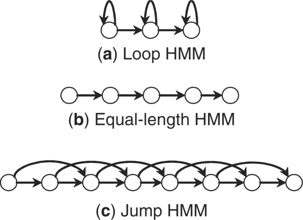
The emission distribution of gene expression in each state is modeled by a multivariate Gaussian distribution whose dimension equals the number of genes used by the classifier. To avoid overfitting, the covariance matrix is assumed to be diagonal. We considered three state space topologies, all being left-right models that conform to the temporal ordering as shown in Figure 1. The first topology is a left-right model with self-loops, i.e. a state indexed i has transitions to i or i+1. The second is a simple left-right model without loops or jumps, so each state exactly matches one time point. The third is a left-right model with jumps, i.e. a state i has transitions to i+1,i+2,…,i+J, where the maximum jump step J is a fixed constant. In the first topology the number of states is less than the number of time points, while in the second topology these two are equal, and in the third topology the number of states is larger than the number of time points. The first and third topologies can be used to align patients by modifying their transition probabilities based on the observed expression data.

Fig. 1.

Three HMM topologies considered in this article. All three are left-right models that conform to temporal ordering. (a): left-right models with self-loops (less states than time points); (b): left-right models without loops or jumps (equal number of states and time points) and (c): left-right models with jumps (more states than time points).

We will use the following notations. We are given the time series gene expressions of K patients, {O₁,O₂,…,O_K}. We measure the expression of G genes for each patient at T time points, represented by a G-dimensional multivariate time series O_k = (O_k1,O_k2,…,O_kT). For gene selection, O_ktg denotes the expression of gene g at time t for patient k. The class patient k belongs to is denoted as c_k, c_k∈{1,2}. For notational simplicity, we assume the patients are from two classes, which is true for many clinical patient classification tasks. However, the algorithm discussed below is applicable for multiclass classification as well.

A HMM λ^(m) with multivariate Gaussian emission probability is trained for each class m, m∈{1,2}. Let

where is the transition probability from state i to j and are mean and SD for the Gaussian distribution of state j. The mean and SD of gene g in state j is denoted as and , when it is necessary to specify which gene. We fix the first state for each topology to represent pre-treatment levels. The hidden states of time series O_k are denoted as x_k=(x_k1,x_k2,…,x_kT).

We also use the standard notation for the sufficient statistics of HMM: is the posterior probability of state j at time t of observation O_k, conditioned on the model λ^(m). is the probability of a transition from state i to state j at time t of observation O_k, conditioned on the model λ^(m).

2.1 Generative training of HMM

Given labeled expression data we can learn the parameters of a HMM using the Baum–Welch algorithm for each of the three topologies mentioned above. The resulting models are generative as training only utilize data from expression experiments of patients which belong to that class (good or poor responders). Using such a generative model we can classify a new dataset by building one model for each class. Class assignment is based on maximum conditional likelihood.

It has been shown that MLE is optimal if the true model is indeed the assumed HMM and there is infinite data (Nadas, 1983). Unfortunately, it is unlikely that the data is truly generated by a HMM. Furthermore, the number of training examples for clinical time series classification is very small. Thus, it would be beneficial if we could take advantage of both positive and negative data when building the models for each of the classes. This would allow the models to focus on the differences between the two sets of expression datasets, rather than on the most visible features (which could be the same for all groups of patients, for example stress response which is a common feature in disease response but may not be a useful feature for discriminating good and bad responders).

2.2 Discriminative training of HMM

To model the difference between positive and negative examples, we need to optimize a discriminative criteria, such as the conditional likelihood of the true classes given the data. This criteria is also called conditional maximum likelihood estimation (CMLE), often used in discriminative training methods, e.g. logistic regression. Here we use the MMIE technique which was originally developed for speech recognition, to trains HMMs in order to optimize this discriminative criteria. The standard training algorithm for MMIE is an extended version of the Baum–Welch algorithm (Gopalakrishnan et al., 1991). However, unlike generative training, the HMMs for both classes are learned concurrently and parameters in one of the models are affected by the parameters estimated for the other model. The MMIE objective function can be written as,

(1)

Where c_k is the class (1 or 2) of patient k.

That is, our goal is to find parameters that will maximize the probability ratio of the good and poor responders models.

The denominator in Equation (1) will be represented by the likelihood of a combined HMM, λ^den, such that

λ^den is called the denominator model. In practice we learn new models for p(λ⁽¹⁾) and p(λ⁽²⁾) in each iteration and use them to revise p(O_k|λ^den). Thus the denominator model is constructed by combining the state space of the two HMMs λ⁽¹⁾ and λ⁽²⁾, and assigning initial probability to the beginning states according to the priors p(λ⁽¹⁾) and p(λ⁽²⁾). During training, the denominator model is constructed in each iteration after the HMMs λ⁽¹⁾ and λ⁽²⁾ are updated. While updating one class, the HMM for that class is called the numerator model.

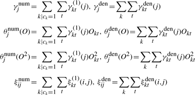
We first discuss the E-step in MMIE which involves the estimation of expected counts summarizing the current parameter settings. This estimation is similar to the ones in the Baum–Welch algorithm and the counts are collected for both the numerator and denominator models. For example, when λ⁽¹⁾ is being updated, is the expected count of state j in the positive examples according to the numerator model λ⁽¹⁾; is the expected count of transition from state i to state j in the positive examples according to λ⁽¹⁾. are weighted sums of expression values in the positive examples, and are weighted sums of squared values, where the weightings are the posterior probability of state j. Similarly, and are expected counts in all examples according to the denominator model λ^den. The calculations when updating λ⁽²⁾ is similar. These expected counts are obtained from the dynamic matrices of the forward–backward algorithm. Formally,

The major difference between generative and discriminative HMMs is in the M-step. MLE for the generative model only updates the parameters in the direction of positive examples, e.g. . In contrast, MMIE updates the parameters by moving them toward the positive examples and away from the denominator model. This leads to greater focus on emission and transition probabilities that differ between the two models (either across states or at specific states for each gene) contributing to increased discrimination between the two models. However, such subtraction may generate negative transition probabilities or negative variances in emission probabilities. A smoothing constant needs to be added to both the numerator terms and the denominator terms to avoid this. Hence the reestimation formulas of MMIE are,

(2)

(3)

(4)

where D_E and D_T are smoothing constants for emission and transition probabilities, respectively.

It has been shown that Equation (2)–(4) will converge to a local maximum of the MMIE objective function, given sufficiently large smoothing constants D_E and D_T (Normandin et al., 1994). However, it is not known how large they must be for the objective function to converge. If the smoothing constants are too small, update may not increase the (discriminative) objective function, but if they are too large, convergence will be too slow. A useful lower bound is the minimal values that ensures that the HMM parameters remain valid. Empirically, setting the smoothing constants to twice the lower bound leads to fast convergence (Woodland and Povey, 2002). Thus we set D_E to twice the minimal value that makes all variances positive; D_T is set to twice the minimal value that makes all transition probabilities positive. See Appendix A for details on how these values can be computed.

The HMM parameters are updated by a weighted average of the previous parameters and the reestimations. We follow previous works and set the learning rate, the weight of reestimations, as the error rate (Normandin et al., 1994). Hence the learning rate is larger in the beginning and smaller when nearing convergence.

3 GENE SELECTION FOR TIME SERIES EXPRESSION CLASSIFICATION

Gene selection is critical in clinical gene expression classification for several reasons. First, the number of patients (data points) is small compared to the number of genes (features), resulting in overfitting. It is expected that restricting to a subset of relevant genes will improve classification accuracy. Second, a small subset of genes that discriminate between the classes can lead to biomarker discovery. The selected genes can be further examined by more experiments to find out the causal factors of different response to a treatment.

We consider the problem of gene selection as a feature selection problem and will use the terms ‘gene’ and ‘features’ interchangeably. There are two primary approaches for feature selection; the ‘wrapper’ approach and the ‘filter’ approach (Xing, 2002). The wrapper approach evaluates the classifier on different feature subset, and searches in the space of all possible feature subsets using the specific classification strategy. The filter approach does not rely on the underlying classifier, but instead uses a simpler criteria to filter out irrelevant features. Typically the filter approach is faster, while the wrapper approach can fit the specific need of a classifier and obtain better performance. In pursuit of higher classification accuracy, the feature selection method we used here is a wrapper method.

We used a backward stepwise feature selection method that utilizes the alignment to the HMM profiles based on recursive feature elimination (RFE) algorithm, termed HMM–RFE (Guyon et al., 2002). The basic procedure of RFE is as follows: train the classifier, eliminate the feature whose contribution to the discrimination is minimal, and repeat iteratively until the stopping criteria is met. It is also possible to eliminate several features in one step, especially when the number of features is large.

To estimate the contribution to discrimination of a specific gene, we note that since the covariance matrix is diagonal, gene-expression levels are independent given the hidden states. Thus, if the states are known, the likelihood can be decomposed into terms involving each gene separately. However, such a decomposition does not exist when the hidden states are unknown. Instead we use a heuristic to approximate this decomposition.

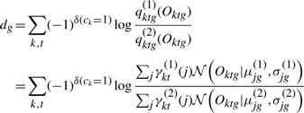
We define the contribution to log odds of a gene g, d_g, as

(5)

where δ(c_k=1) is 1 if c_k=1 and 0 otherwise. See Appendix B for a detailed derivation. Briefly, the equation above uses an estimate of the states ( and ) to compute the discriminative contribution of genes for the two classes.

In each selection step, genes are ranked by the contribution d_g, and the gene with lowest score is eliminated. Following the elimination step, new HMMs are trained using the remaining genes and the gene selection step is repeated.

In order to determine the final number of selected genes we use internal cross-validation within the training data. Note that internal cross-validation does not utilize the test data in any way. The HMM-RFE algorithm is summarized in the following procedure:

1. Given G genes, define gene sets with a decreasing number of genes, G=G₀>G₁>G₂>···>G_N, such that G_i genes are selected at the i-th iteration. Initially, the active gene set includes all genes, and i=0.

2. At i-th selection, train the HMMs λ⁽¹⁾ and λ⁽²⁾ using genes in the active gene set.

3. Calculate the discrimination score d_g for each gene g, using Equation (5). Select G_i genes with highest scores.

4. Record the cross-validation accuracy of the active gene set.

5. Set i←i+1, repeat Step 2 until i=N−1.

6. Choose the optimal gene number G^* leading to the highest cross-validation accuracy.

Although we use internal cross-validation to determine the optimal gene set, it is not used in gene ranking. The reason is computational. Internal cross-validation for genes would increase the complexity by a factor of G (total number of genes) which could be a substantial increase for microarray expression data measuring thousands of genes.

4 RESULTS

We first tested our method on simulated data. Next, we applied our method to a clinical dataset measuring MS patients’ response to IFNβ, one of the most common treatments to control MS.

4.1 Simulated dataset

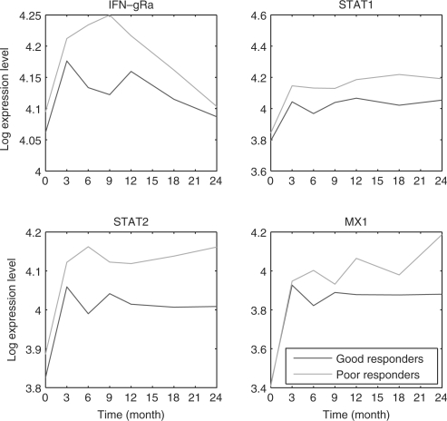
The expression of genes in response to treatments often follows a bifurcating pattern diverging as time progresses (Ernst et al., 2007). This is also the case in clinical settings, as can be seen in Figure 2. In that figure we plot the average expressions of four genes in MS patients treated with IFNβ (Baranzini et al., 2005). The patients are divided into two groups, good and poor responders (red and green curves, respectively). As the figure indicates, while these genes display similar levels at the early time points they diverge at the later time points. A classifier that only utilizes the first time point is likely to perform much worse when compared to a classifier that utilizes the entire time series.

Fig. 2.

Averaged log expression of good and poor responders for four bifurcating genes. Expression levels are absolute difference and not log ratios to the first time point.

To generate the simulated data we have also tried to mimic this type of expression pattern as we describe below. We generated expression profiles for 100 patients. Of these, 50 patients were in class 1 (‘good responders’) and 50 in class 2 (‘poor responders’). 100 genes were measured for each patients, with a maximum of 8 time points per patient. For each gene g, we generated the Class 1 response profile by randomly selecting a segment of a sine wave, of length 1.5π between 0 to 4π. Denote this profile as a function, . We selected 10 out of the 100 genes to be differential, the other 90 where assigned the same values for Class 2. For differential genes, the gene-expression profile of poor responders is the good responders’ profile curve plus a piecewise linear function,

where the gradient a_g and the offset b_g are gene-specific parameters. a_g is +5 or −5, and b_g is uniformly selected at random between −0.1 and 0.3.

After the profiles are generated, we simulate patient-specific response rate by randomly choosing a scaling value s_k between 0.5 to 1.5 for patient k. s_k is used to transform the time series for patient k by stretching or shrinking the curves. Thus, the time series profile for each genes of patient k is the linearly scaled profile time series. Finally, we add Gaussian noise, with mean 0 and gene-specific variance . Formally,

We tried a number of different values for based on real datasets and all resulted in similar performance.

We compared our HMM-based classification with two baseline classifiers: linear SVM (default parameters of SVM light is used), and the Integrated Bayesian Inference System (IBIS) method of Baranzini et al. (2005). IBIS only uses the first time point as we discussed in Section 1.1. We note that we have tried to obtain the code for the Kalman filter SVM of Borgwardt et al. (2006) for direct comparison. Unfortunately, the code is not available online. Despite several e-mail requests we were unable to obtain their code and we thus cannot present direct comparison of the two methods.

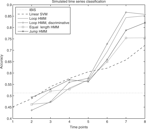
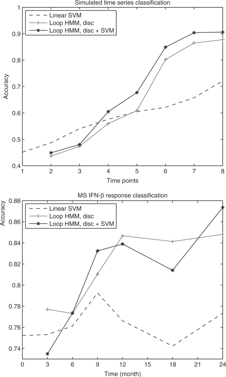
Classification accuracy of different methods are shown in Figure 3. Due to large amount of noise and limited information at earlier time points, classification using data from these points is close to random, causing difficulties for IBIS. With more time points, HMMs provide satisfactory results. HMMs using the three topologies all outperform SVM from 6 to 8 time points. Overall, the loop model results in highest accuracy with more time points.

Fig. 3.

Classification accuracy of simulated data, based on five random permutations and 4-fold cross-validation (20 different training–testing splits). For the loop HMM, 2 to 4 time points use 1 state, 5 to 7 time points use 2 states, and 8 time points use 3 states. For the jump HMM, 4, 5, 6, 8, 10, 10 and 12 states are used from 2 to 8 time points. For both loop and jump HMM, 10 random initialization are carried out and the initialization with the highest likelihood is chosen.

For the loop HMM, we performed discriminative training on the HMMs trained generatively after gene selection. Although it is possible to incorporate discriminative training in HMM–RFE, the computation would be much heavier because discriminative training requires more iterations (e.g. 500 iterations) to converge comparing to generative training (about 20 iterations). As can be seen, accuracy is higher except for 2 time points where classification is close to random. Hence discriminative training can further improve the performance as it utilize both positive and negative data.

We also verified whether gene selection found the true differential genes. Since different splits results in different gene selection, we listed the median number of selected genes, and verified the correctness of overlapping genes: genes selected in 90% of the splits, in Table 1. Note that all overlapping genes are correct after 5 time points, and the number of selected genes is small after 6 time points, especially when using 7 and 8 time points resulting in better accuracy.

Table 1.

Selected genes in simulated data

Time	Accuracy (%)	Median	Number of overlapping genes	Precision of selected genes (%)
2	44	19	1	0
3	47	18	2	0
4	56	16	2	0
5	58	17	2	100
6	73	7	2	100
7	87	2	1	100
8	86	4	2	100

Time is the number of time points used to construct the HMM model. Accuracy is the best accuracy using these time points (loop HMM using discriminative training). Median is the median number of selected genes. Number of overlapping genes presents the number of genes selected in at least 90% of the training–testing splits. Precision is the percent of overlapping genes that were indeed part of the 10 assigned differentially expressed genes.

4.2 MS dataset

We next tested our model using a clinical expression dataset. This dataset contains time series expression data for 70 genes in 52 MS patients treated with IFNβ Baranzini et al. (2005). Of the 52 patients, 33 responded well to the treatment (‘good responders’) and 19 did not respond well (‘poor responders’). The 70 genes included were preselected by experts based on relevance to MS. For each patient there are 7 time points, measured every 3 month in the first year following treatment and every 6 month in the second year. Some patients miss certain measurements, especially at the 7th time point, causing an entire measurement to be a missing value.

As we did with the simulated data, we compared our method to the original IBIS algorithm and to linear SVM. We note again that we were unable to compare our method to the Kalman filter SVM of Borgwardt et al. (2006) since we could not obtain their code.

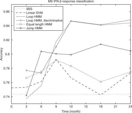
The classification accuracy is evaluated using 4-fold cross-validation. For each possible number of time points (2, 3, etc.) we train a new instance of each potential classification model (SVM, HMMs, etc.). Figure 4 presents the results. In that figure we plot the accuracy versus. the number of time points for the different classifiers.

Fig. 4.

Classification accuracy of MS patients’ response to IFNβ, based on 5 random permutations and 4-fold cross validation (20 different training-testing splits). For the loop HMM, 2 and 3 time points use 1 state, 4 to 6 time points use 2 states, and 7 time points use 4 states. For the jump HMM, 3, 4, 7, 8, 10, 12 states are used from 2 to 7 time points. For both loop and jump HMM, 10 random initialization were carried out and the initialization resulting in the highest likelihood was selected.

As can be seen, HMM with equal number of states and time points (equivalent to Gaussian Naive Bayes classifier) achieves classification accuracy that is similar to SVM with default parameters (tuning of SVM parameters improves the accuracy, but it is still significantly lower than the other HMMs). In contrast, the other two HMMs that allow for alignment perform much better on this clinical dataset, indicating the alignment is indeed an important issue for time series classification. The loop HMM model performs better than the jump model from 3 time points; a possible explanation is that fewer emission parameters reduced overfitting. The best results when using all data (7 points) were obtained by the loop HMM after discriminative training (85%). In addition, when using 2 or 3 time points the discriminative HMM outperformed the generative model. However, for the other sets of time points the two models (discriminative and generative) achieved similar results.

It is important to note that we do not use the test data in gene selection during training, so that the evaluation would be closer to the performance on new data. The results presented in Figure 4 differ from the results in the original IBIS paper (Baranzini et al., 2005) even though we have followed exactly the same (and simple) procedure as described in that paper. We believe that the reason for this discrepancy is that, while exhaustive search of all triplets and full covariance matrix in IBIS gives very good results on the training data, it may lead to overfitting of the validation accuracy, which becomes much higher than test accuracy.

4.3 Selected genes and the advantages of patient alignment

We next examined the selected genes for the different classifiers (trained with different number of time points). Table 2 lists the selected genes for models constructed from the different sets of time points. Again we only list genes selected in at least 90% of the training–testing splits. With more time points the classifiers stabilize between splits leading to more selected genes. We compared our list to a previous list of 12 genes selected by Baranzini et al. (2005) based on expression values prior to treatment (first time point). Caspase 10 and Caspase 3 which were also listed in the original paper, are almost always selected regardless of how many time points are being used. However Jak2, IL12Rb2 and RAIDD are only selected using more time points, and are not on the list of 12 genes in that paper.

Table 2.

Selected genes in MS dataset

Time	Accuracy (%)	Median	Selected genes
2	78	15	Caspase 3, Caspase 10, IL-4Ra
3	77	13.5	Caspase 3, Caspase 10, Jak2
4	81	11.5	Caspase 10, Caspase 2, Jak2
5	85	26	Caspase 10, MAP3K1, IRF8, Caspase 3,
			Caspase 2, Jak2, IL-4Ra, IL12Rb2
6	84	13.5	Caspase 10, Caspase 3, Jak2, IRF4,
			Caspase 2
7	85	23.5	Caspase 10, Caspase 3, Jak2, IL-4Ra,
			MAP3K1, RAIDD, Caspase 2

See Table 1 for description of the time, accuracy and median columns. Selected genes are genes selected in at least 90% of the training–testing splits. Accuracy is based on loop HMM using discriminative training.

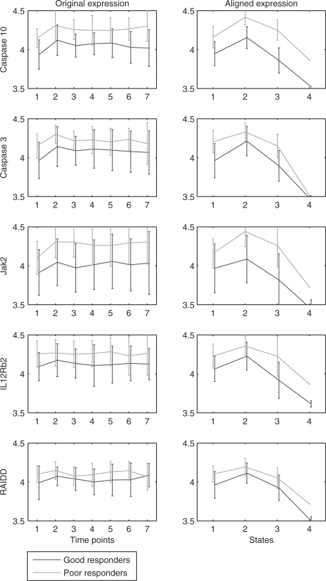
These uniquely selected genes are due to the ability of our method to consider later time points, as shown in Figure 5. The left column in Figure 5 plots the mean and variance of gene expression at different time points. Some genes like Jak2 differs in later time points more strongly between the two classes when compared to the first time point. For some genes, the divergence is visible only in the aligned expression models, shown in the right column of Figure 5. To obtain the aligned expression, we use the Viterbi algorithm to align the time points of a patient to the most likely states of the HMM. IL12Rb2 and RAIDD, for example, are more separated between classes in the aligned expression. The large variances (and hence overlap) in unaligned time series could be due to poor responders entering the third state earlier or good responders staying in the second state longer, which is resolved after the alignment. Note that the alignment is on the patient level, based on the expression of all genes. To isolate the effect of alignment we applied a linear SVM to the alignment model determined by the HMM. Unlike the regular SVM that uses the measured values, the alignment SVM uses the average expression of time points aligned to each of the HMM states. As Figure 6 shows, such a classifier leads to much higher accuracy than SVM based on unaligned expressions. However, while this classifier considers the alignment, it ignores the temporal ordering of the states which is why it is outperformed by discriminative HMM, at least in some cases. These results highlight the importance of alignment when working with clinical expression data.

Fig. 5.

Mean and variance of expression profiles of unaligned and aligned genes selected for models using 5 or more time points. Plots in the same row are for the same gene. The right column presents, for each of the genes, the aligned expression profiles corresponding to the four states using the Viterbi algorithm. Alignment is based on the best discriminative HMM of all training–testing splits. In the learned model, the selected genes go up in the second state and back to initial level in the third state. The fourth state basically models outliers in the 6th and 7th time point, and hence transition probability into this state is small. The overlap between classes on the second and third states of all the five genes is smaller after the alignment leading to better discrimination between poor and good responders. This is critical for the correct identification of IL12Rb2 and RAIDD as two important features for later time points.

Fig. 6.

Applying SVM to the averaged expressions of aligned time points. The alignments are obtained by running the Viterbi algorithm on the best discriminative HMM. The SVM uses the linear kernel and default parameters.

Some of the genes we uniquely identified are also validated by recent complementary studies. IL12RB2, an important autoimmunity gene is expressed in activated T-cells and is a marker of TH1 inflammatory response. Its consistent increase in poor responders suggests lack of response to treatment. This becomes more evident as time goes by leading to maximal difference after a year (Fig. 5). A recent paper found that it was a good marker for lack of response to glatiramer acetate in MS (Grossman et al., 2007), and as our results indicate it might be a good marker to the IFNβ treatment. Another genes we identified, JAK2, is phosphorylated by the activation of the IL12 receptor. Again, this might cause a delayed response leading to stronger differences at later time points.

5 DISCUSSION

A major challenge in classifying time series clinical expression data is the varying response rates of individuals. In this article we propose the use of HMMs for this task. HMMs can naturally model non-linear patient-specific response rates. The hidden states represent the temporal clustering of gene expression, and can be interpreted as disease phases. Transition probabilities allows different patients to progress at different rates. To overcome the small number of training examples we have used discriminative HMMs. Unlike generative HMMs, discriminative HMMs can utilize both positive and negative examples when generating a model for each class.

Using both simulated data and clinical expression data of MS patients, we show that HMMs outperforms classifiers that do not take the temporal ordering into account. We further compared three left-right HMM models: the loop model, the equal-length model, and the jump model. Of these, the loop model performs best which is likely the result of the small training data for these types of experiments. Discriminative HMMs improve upon generative HMMs in most, though not all, cases.

In addition to learning discriminative models we also carry out gene selection. The selected genes in simulated datasets correctly contain the truly differential genes. While we do not have the ground truth for the MS dataset, many of the selected genes can be explained based on current knowledge of disease progression.

As more time series expression data accumulates we would like to test our method on additional types of response data. We would also like to extend our model to better represent the interactions between genes. The current diagonal covariance emission model ignores such interactions. When more data becomes available, models that compute more covariance terms can be learned from data leading to better models and improved accuracy. We are also interested in other clinical applications of our HMM, e.g. predicting rejection events for transplant patients. Alignment of time series gene expression between group of genes or species could also be important in other biological experiments.

APPENDIX A

For discriminative training of HMM using MMIE, the smoothing constants are set to twice the minimal value that ensures the probabilities to be valid. Here we show how to calculate the D_T and D_E smoothing constants for transition and emission probabilities, respectively. By setting in Equation (4) to be positive, D_T can be calculated as

By plugging Equation (2) into Equation (3) and setting to be positive, we have a quadratic inequality of D_E,

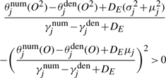or

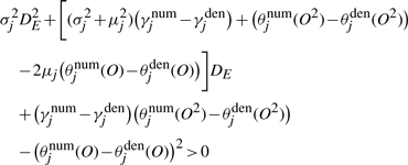This quadratic inequality can be solved to obtain a lower bound, and D_E is set to twice the lower bound.

APPENDIX B

In gene selection, we need to estimate the contribution to discrimination of each gene. Because the covariance matrix is diagonal, the gene expressions are independent given the hidden states. That is, the probability of a time series gene expression O_k given a HMM λ⁽¹⁾ and the hidden states x_k can be decomposed as,

What we need is to decompose the marginalized likelihood p(O_k|λ⁽¹⁾) into terms involving each gene only, :

Unfortunately, expressions levels for individual genes are not independent once the hidden state are not known, so the above decomposition does not exist. We will use a heuristic to approximate this decomposition. Since the hidden states are unknown, we approximate it by the posterior probabilities, . We approximate the term as the weighted average of the Gaussian emission probabilities, the weights being :

We can approximate the contribution of each gene to the log odds,

Then the total log odds of the correct model versus the incorrect model can be expressed as the sum of contribution of each gene, d_g,

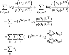where δ(c_k=1) is 1 if c_k=1 and 0 otherwise. Thus we have contribution to log likelihood ratio of a gene d_g, defined as

REFERENCES

- Aach J, Church GM. Aligning gene expression time series with time warping algorithms. Bioinformatics. 2001;17:495–508. doi: 10.1093/bioinformatics/17.6.495. [DOI] [PubMed] [Google Scholar]
- Alizadeh A, et al. Distinct types of diffuse large b-cell lymphoma identified by gene expression profiling. Science. 2000;403:503–510. doi: 10.1038/35000501. [DOI] [PubMed] [Google Scholar]
- Bar-Joseph Z, et al. Continuous representations of time series gene expression data. J.Comput.Biol. 2003;3–4:341–356. doi: 10.1089/10665270360688057. [DOI] [PubMed] [Google Scholar]
- Baranzini SE, et al. Transcription-based prediction of response to IFNbeta using supervised computational methods. PLoS Biol. 2005;3:e2. doi: 10.1371/journal.pbio.0030002. [DOI] [PMC free article] [PubMed] [Google Scholar]
- Bicciato S, et al. Pca disjoint models for multiclass cancer analysis using gene expression data. Bioinformatics. 2003;19:571–578. doi: 10.1093/bioinformatics/btg051. [DOI] [PubMed] [Google Scholar]
- Borgwardt KM, et al. Maui, HI: 2006. Class prediction from time series gene expression profiles using dynamical systems kernels. In; pp. 547–558. Proceedings of Pacific. Symposium on Biocomputing (PSB) [PubMed] [Google Scholar]
- Ernst J, et al. Reconstructing dynamic regulatory maps. Mol. Syst. Biol. 2007;3:74. doi: 10.1038/msb4100115. [DOI] [PMC free article] [PubMed] [Google Scholar]
- Furey T, et al. Support vector machine classification and validation of cancer tissue samples using microarray expression data. Bioinformatics. 2000;16:906–914. doi: 10.1093/bioinformatics/16.10.906. [DOI] [PubMed] [Google Scholar]
- Golub T, et al. Molecular classification of cancer: class discovery and class prediction by gene expression monitoring. Science. 1999;286:531–537. doi: 10.1126/science.286.5439.531. [DOI] [PubMed] [Google Scholar]
- Gopalakrishnan P, et al. An inequality for rational functions with applications to some statistical estimation problems. IEEE Trans. Inf. Theory. 1991;37:107–113. [Google Scholar]
- Grossman I, et al. Pharmacogenetics of glatiramer acetate therapy for multiple sclerosis reveals drug-response markers. Pharmacogenet. Genomics. 2007;17:657–666. doi: 10.1097/FPC.0b013e3281299169. [DOI] [PubMed] [Google Scholar]
- Guyon I, et al. Gene selection for cancer classification using support vector machines. Mach. Learn. 2002;46:389–422. [Google Scholar]
- [(last accessed date 15 January 2008)];Inflammation and the Host Response to Injury. 2008 Inflammation, Available at: www.gluegrant.org.
- Kaminski N, Bar-Joseph Z. A patient-gene model for temporal expression profiles in clinical studies. J. Comput. Biol. 2007;14:324–338. doi: 10.1089/cmb.2007.0001. [DOI] [PubMed] [Google Scholar]
- Listgarten J, et al. Neural Information Processing Systems 17. Cambridge, MA: MIT Press; 2004. Multiple alignment of continuous time series; pp. 817–824. [Google Scholar]
- Nadas A. A decision theoretic formulation of a training problem in speech recognition and a comparison of training by unconditional versus conditional maximum likelihood. IEEE Trans. Acoust. Speech Signal Process. 1983;31:814–817. [Google Scholar]
- Normandin Y, et al. High-performance connected digit recognition using maximum mutual information estimation. IEEE Trans. Speech Audio Process. 1994;2:299–311. [Google Scholar]
- Nutt C, et al. Gene expression-based classification of malignant gliomas correlates better with survival than histological classification. Cancer Res. 2003;63:1602–1607. [PubMed] [Google Scholar]
- Schliep AP, et al. Analyzing gene expression time-courses. IEEE/ACM Trans. Comput. Biol. Bioinform. 2005;2:179–193. doi: 10.1109/TCBB.2005.31. [DOI] [PubMed] [Google Scholar]
- Sterrenburg E, et al. Large-scale gene expression analysis of human skeletal myoblast differentiation. Neuromuscul. Disord. 2004;14:507–518. doi: 10.1016/j.nmd.2004.03.008. [DOI] [PubMed] [Google Scholar]
- van 't Veer LJ, et al. Gene expression profiling predicts clinical outcome of breast cancer. Nature. 2002;415:530–536. doi: 10.1038/415530a. [DOI] [PubMed] [Google Scholar]
- Weinstock-Guttman B, et al. Genomic effects of IFN-beta in multiple sclerosis patients. J. Immunol. 2003;171:2694–2702. doi: 10.4049/jimmunol.171.5.2694. [DOI] [PubMed] [Google Scholar]
- Woodland P, Povey D. Large scale discriminative training of hidden markov models for speech recognition. Comput. Speech Lang. 2002;16:25–47. [Google Scholar]
- Xing E. Feature selection in microarray analysis Ch.6. In. In: Berrar D, et al., editors. A Practical Approach to Microarray Data Analysis. London: Kluwer Academic Publishers; 2002. pp. 110–131. [Google Scholar]
- Yoneya T, Mamitsuka H. A hidden markov model-based approach for identifying timing differences in gene expression under different experimental factors. Bioinformatics. 2007;23:842–849. doi: 10.1093/bioinformatics/btl667. [DOI] [PubMed] [Google Scholar]