Identifying functional modules in protein–protein interaction networks: an integrated exact approach

Abstract

Motivation: With the exponential growth of expression and protein–protein interaction (PPI) data, the frontier of research in systems biology shifts more and more to the integrated analysis of these large datasets. Of particular interest is the identification of functional modules in PPI networks, sharing common cellular function beyond the scope of classical pathways, by means of detecting differentially expressed regions in PPI networks. This requires on the one hand an adequate scoring of the nodes in the network to be identified and on the other hand the availability of an effective algorithm to find the maximally scoring network regions. Various heuristic approaches have been proposed in the literature.

Results: Here we present the first exact solution for this problem, which is based on integer-linear programming and its connection to the well-known prize-collecting Steiner tree problem from Operations Research. Despite the NP-hardness of the underlying combinatorial problem, our method typically computes provably optimal subnetworks in large PPI networks in a few minutes. An essential ingredient of our approach is a scoring function defined on network nodes. We propose a new additive score with two desirable properties: (i) it is scalable by a statistically interpretable parameter and (ii) it allows a smooth integration of data from various sources.

We apply our method to a well-established lymphoma microarray dataset in combination with associated survival data and the large interaction network of HPRD to identify functional modules by computing optimal-scoring subnetworks. In particular, we find a functional interaction module associated with proliferation over-expressed in the aggressive ABC subtype as well as modules derived from non-malignant by-stander cells.

Availability: Our software is available freely for non-commercial purposes at http://www.planet-lisa.net.

Contact: tobias.mueller@biozentrum.uni-wuerzburg.de

1 INTRODUCTION

Construction and analysis of large biological networks have become major research topics in systems biology (Aittokallio and Schwikowski, 2006). Various aspects have been analyzed including the inference of cellular networks from gene expression (Friedman, 2004), network alignments (Flannick et al., 2006; Kelley et al., 2003; Sharan and Ideker, 2006) and other related strategies as reviewed by Srinivasan et al. (2007). At the same time, well-established microarray technologies provide a wealth of information on gene expression in various tissues and under diverse experimental conditions. Integrating protein–protein interaction (PPI) and gene-expression data generates a meaningful biological context in terms of functional association for differentially expressed genes.

Frequently, large scale expression profiling studies investigate many experimental conditions simultaneously, thereby generating multiple P-values. Especially in tumor biology expression profiling has become a well-established tool for the classification of different tumors and tumor subtypes. Furthermore, in the clinical context, various patient-associated data are available that—in conjunction with expression data—provide valuable information of the influence of specific genes on disease-specific pathophysiology. In particular the analysis of survival data allows to establish gene expression signatures to make predictions about the prognosis and to assess the disease relevance of certain genes. However, the cellular function of an individual gene cannot be understood on the level of isolated components alone, but needs to be studied in the context of its interplay with other gene products. The combined analysis of expression profiles and PPI data thus allows the detection of previously unknown dysregulated modules in interaction networks not recognizable by the analysis of a priori defined pathways.

Ideker et al. (2002) have proposed to identify interaction modules in this setting by devising firstly an adequate scoring function on networks and secondly an algorithm to find the high-scoring subnetworks. The underlying combinatorial problem has been proven to be NP-hard for additive score functions defined on the nodes of the network. The authors proposed a heuristic strategy based on simulated annealing and developed a score to measure the significance of a subnetwork that includes the integration of multivariate P-values. This score has been extended by Rajagopalan and Agarwal (2005) to incorporate an adjustment parameter in order to obtain smaller subgraphs in conjunction with a greedy search algorithm. This approach however, excludes the possibility to combine multiple P-values. Variants of greedy search strategies have also been used by Nacu et al. (2007) and Sohler et al. (2004). Subsequently Cabusora et al. (2005) proposed an edge score by adapting the scoring concept of Ideker et al. (2002). An alternative edge scoring based on correlation of gene expression has been proposed by Guo et al. (2007). All the former methods are heuristic approaches that cannot guarantee to identify the maximally scoring subgraph. Some of these often computationally demanding approaches tend to deliver large high-scoring networks, which may be difficult to interpret.

Here we present a novel approach (i) that is characterized by a modular scoring function, based on signal-noise decomposition implemented as a mixture model, (ii) permits the smooth integration of multivariate P-values derived from various sources, (iii) delivers provably optimal and suboptimal solutions to the maximal-scoring subgraph problem by integer-linear programming (ILP) in reasonable running time and (iv) allows to control the resultant subnetwork size by an adjustment parameter, which is statistically interpretable as false-discovery rate (FDR).

The presented algorithm is, to our knowledge, the first approach that really tackles and solves the original problem raised by Ideker et al. (2002) to optimality. We strongly believe that the optimal and suboptimal solutions produced by our method provide a considerable benefit over heuristic solutions in that they allow for a sound evaluation and adaptation of the underlying model. Given only a heuristic solution it is impossible to decide whether poor results are due to inappropriate parameter settings or due to the optimality gap. Based on extensive simulations we evaluate our exact approach in comparison to the heuristic method proposed by Ideker et al. (2002). Finally, analyzing a comprehensive microarray and survival dataset of lymphoma patients we detect functional modules, extending the results of Rosenwald et al. (2002).

The remainder of this article is organized as follows: after describing the data and methods we use (Section 2), we introduce our approach and its application to lymphoma interactome data in Section 3. Section 4 presents the subnetworks we found and a validation of our approach in comparison to the method by Ideker et al. We conclude with Section 5, where we discuss our findings.

2 METHODS

2.1 Microarray and survival data

We used the published gene-expression data set from diffuse large B-cell lymphomas (DLBCL) (Rosenwald et al., 2002). In particular, gene expression data from 112 tumors with the germinal center B-like phenotype (GCB DLBCL) and from 82 tumors with the activated B-like phenotype (ABC DLBCL) were included in this study. Gene expression analysis was performed on the Lymphochip including 12 196 cDNA probe sets (Rosenwald et al., 2002). In addition, survival information was available from 190 patients (Rosenwald et al., 2002).

Statistical analyses were performed using the software package R (R Development Core Team, 2006) and Bioconductor (Gentleman et al., 2004) and the routines implemented in limma (Smyth, 2004). For normalization of gene expression within arrays we used the loess method, normalization between arrays was performed by using the scale method to adjust the log ratios to the same median absolute deviation (MAD) across arrays as detailed in Blenk et al. (2007). For subsequent analyses the expression values for different spots of the same gene have been aggregated by taking the median. Significance of differential expression between the two subtypes ABC and GCB was calculated using robust statistics based on linear models and a moderated t-test (Smyth, 2004). Survival analysis was performed by Cox regression as implemented in the R-package survival (Andersen and Gill, 1982; Therneau et al., 1990).

2.2 Network

The dataset of literature-curated human PPI has been obtained from HPRD (Mishra et al., 2006; Peri et al., 2003). Using R and the network structures and algorithms in the Bioconductor packages graph and RBGL (Carey et al., 2005), we derived an interactome network consisting of 36 504 interactions between 9392 different proteins. With the subset of genes shared between the interactome dataset and the chip a Lymphochip-specific interactome network was derived as the vertex-induced subgraph. The resulting network comprises 2561 different gene products and 8538 interactions, with a large connected component of 2034 proteins (79.4%) and 8399 interactions (98.4%). The remaining proteins were either non-interacting singletons (472) or tiny clusters of sizes between two and six (23). Our analysis focuses exclusively on the giant connected component. visualization and further network analysis was performed with Cytoscape (Cline et al., 2007; Shannon et al., 2003).

2.3 Optimization algorithm

Our algorithm is based on the software dhea (district heating) from Ljubić et al. (2006). We have extended the C++ code in order to generate suboptimal solutions and have created several Python scripts to control the transformation to a Steiner tree problem, the use of dhea and the re-transformation to a PPI subnetwork. The dhea code uses the commercial CPLEX callable library version 9.030 by ILOG, Inc. (Sunnyvale,CA) (Sunnyvale, CA). All experiments were run on a 64 bit 2.2 GHz Opteron Intel with 8 GB of main memory. Our software and the datasets used in this study are publicly available for academic and research purposes within the heinz (heaviest induced subgraph) package of the open source library LiSA (http://www.planet-lisa.net).

3 SCORING FUNCTION AND ALGORITHM

This section introduces our new integrated exact approach to support the identification of functional modules in PPI networks. Section 3.1 focuses on the order statistics-based method to determine score values for the network nodes. We illustrate our approach by analyzing a network obtained by combining the data from a expression profiling study of lymphoma patients (Rosenwald et al., 2002) with the comprehensive interactome data from HPRD (Peri et al., 2003). We derive P-values from the analysis of differential expression between two tumor subtypes (ABC and GCB) as well from the analysis of survival data by Cox regression for each node in the interaction network.

Section 3.2 describes how the score values will be used as input for the maximum-weight connected subgraph (MWCS) problem and a novel algorithmic approach based on mathematical optimization. Our algorithm solves this problem to provable optimality and, furthermore, is able to enumerate sufficiently distinct suboptimal solutions. ▪

3.1 Statistics of scoring function

3.1.1 Aggregation statistics of P-values

Having annotated each node of the interaction network with experimentally derived P-values, we are faced with the problem to aggregate these P-values into one number. A simple aggregation statistics proposed in the literature is the so-called Fisher's method, which combines n P-values p_i by (Fisher, 1948). This method however does not provide the necessary flexibility to control the number of significant P-values, instead it only provides a significance measurement over the entire set of P-values. Due to the heterogeneous nature of the data a more flexible approach is required. Therefore we use an aggregation statistic based on the distribution of the order statistics of P-values. Let X₁,…,X_n be independently identically distributed (iid) then the density of the ith smallest observation X_(i) is given by

(1)

where F(x) denotes the probability density function of X_i, for i=1,…,n (Lindgren, 1993). Now we propose to aggregate the P-values at each node in the network by asking for its ith order statistic of the associated P-values, resulting in one P-value of P-values. Because P-values are uniformly distributed under the null hypothesis (Wasserman, 2005), we apply Equation (1) with density f_X(x)=1 and density function F_X(x)=x and get

(2)

or, in other words, X_(i)∼B(i,n−i+1) with the associated cumulative distribution function

where B(·,·) denotes the beta distribution. Applying Equation (2), each gene in the network can be assigned an overall P-value given by the ith order statistic. This approach is also applicable in case of missing data: for missing P-values the ith order statistic can be used after correcting the parameter n in Equation (2) appropriately.

3.1.2 Signal-noise decomposition

Based on these aggregated P-values we derive our new scoring function. Following Pounds and Morris (2003) we consider the distribution of the P-values as a mixture of a noise and a signal component. The signal is assumed to be B(a,1) distributed whereas the noise is B(1,1)=uniform (0,1) distributed (P-values under the null hypothesis).

The B(a,b) distribution is given by

where Γ(·) denotes the gamma function. Thus the distribution of the derived P-values reduces to

with mixture parameter λ and shape parameter a of the beta distribution. For given data x=x₁,…,x_n the log likelihood is defined as

and consequently the maximum-likelihood estimations of the unknown parameters are given by .

We obtain both parameters by numerical optimization using the L-BFGS-B method (Byrd et al., 1995) as implemented in R. For the lymphoma dataset analyzed here we obtained a value of 0.536 for the mixture parameter λ and 0.276 for the shape parameter a of the beta distribution. This relates to signal and noise proportions of 46.4% versus 53.6%, respectively.

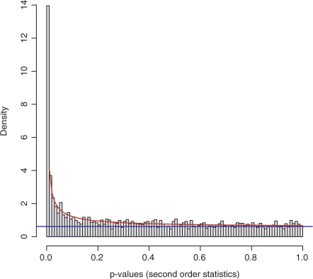
Since P-values are uniformly distributed under the null hypothesis the noise component will be adequately modeled by a uniform distribution. Modeling the signal component by a beta distribution is justified by Figure 1 and a Quantile–Quantile (Q–Q) plot (data not shown). This is furthermore supported by the associated Q–Q plot of the fitted density function with the empirical distribution function, which is extremely close to a straight line (data not shown). These analyses indicate that the signal is well-captured by the beta distribution.

Fig. 1.

The fitted mixture model fits nicely the empirical distribution. The parameters of the mixture model are a=0.276 and λ=0.563. The histogram of the observed P-values displays the strong consistency with the expected densities under the fitted model (red line). The blue line indicates the fraction of P-values derived from the uniform noise model. The excellent fit of the model has been confirmed in a Q–Q plot of the fitted distribution versus the empirical P-value distribution (data not shown).

Our aim is to develop an additive score, where positive values signify signal content and negative values denote background noise. Inspired by the ideas of the likelihood ratio test our approach is as follows: for the fitted parameter a the signal component is equal to the B(a,1) density, whereas that of the noise component is given by B(1,1). Since B(1,1) is equivalent to the uniform distribution the denominator is 1 for the score, which is given by

Obviously for a→1 the density of the signal component converges to that of the background model and consequently the score converges to 0 for all x. In particular even very low P-values will be scored zero. Moreover, for a fitted parameter set a and λ: and . This demonstrates that the score properly combines the parameters a and λ.

Similar to classical hypothesis tests where a certain significance level is proposed, we derive a threshold value that discriminates signal from noise. As detailed in (Pounds and Morris, 2003) the mixture model allows the estimation of the FDR. From this we calculate a threshold P-value τ(FDR), which controls the FDR for the positively scoring P-values. Thus we derive an adjusted log likelihood ratio score given as

(3)

thus adjusted and unadjusted scores differ by an additive offset dependent on the parameter τ. Here, the value τ is the significance threshold. P-values below this threshold are considered to be significant and will score positively whereas those above the threshold are assumed to have arisen from the null model and will be assigned negative scores. It can easily be seen that for τ→0 the score S(x)→−∞ and for τ→1 all scores will be positive and our FDR will be equal to λ, the mixture parameter of the noise model.

Under the null hypothesis, the x_i are iid and the subnetwork score is consequently given by the sum over all protein scores of the subnetwork: , where net denotes the set of all P-values in the network to be scored. Obviously, under this assumption the expectation value of the network score scales linearly with network size. Similar as in the case of local sequence alignments an appropriate choice of the FDR is essential to ensure a negative subnet score to guarantee locality of the solution. Otherwise, however, the optimization would tend to collect as many genes as available to increase the score regardless of an underlying biological signal.

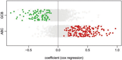
Analyzing our lymphoma network we search for genes that are differentially expressed between the GCB and ABC DLBCL subgroups and, in addition, show an association with overall survival (Fig. 2). To aggregate the derived P-values from gene expression analysis and Cox regression we use the second-order statistic as detailed above. Our score thus combines information about the classification of these tumor subtypes with information about prognosis association. As illustrated in Figure 2 our data contain a strong signal that can be captured by an adequate combination of these two different aspects. Thus, it becomes evident that the ABC subtype characteristically over-expresses genes with an association for a higher risk, whereas in the GCB subtype mainly genes associated with a better prognosis are over-expressed. Hence we search for interaction modules that specifically contribute to the malignant behavior of the ABC subtype as compared to the more benign GCB subtype.

Fig. 2.

Scoring of combined P-values. All genes have been assigned to the ABC and GCB subtype-based fold changes. The x-axis shows coefficients of the univariate Cox proportional hazards regression model fitted for each gene separately. A coefficient greater than zero denotes an increased risk association. Genes scoring positively by our combined scoring function (for a FDR of 0.01) are colored. This evidences that our score selects genes specifically associated with the different malignancy of the two tumor subtypes.

3.2 Mathematical optimization algorithm

Combinatorially, the problem from the previous section can be cast as finding an optimal-scoring subgraph in a vertex-weighted graph:

PROBLEM 1. —

(Maximum-Weight Connected Subgraph Problem, MWCS) Given a connected undirected, vertex-weighted graph G =(V,E,w) with weights w:V→ℝ, find a connected subgraph T=(V_T,E_T) of G, V_T∈V, E_T∈E, that maximizes the score w(T)≔∑_v∈VTw(v).

It is easy to see that any solution for MWCS can always be trimmed to a tree of same weight, and, if all node weights are positive, an optimal solution is easily computed by determining any spanning tree. In case of both positive and negative edge weights, finding the MWCS is not so easy. In fact, in the supplement of Ideker et al. (2002), Karp has shown that MWCS is an NP-complete problem, and the authors use this as a justification for their heuristic search method.

We propose to solve this problem to provable optimality using techniques from mathematical programming. More precisely, we transform the problem into the well-known prize-collecting Steiner tree problem (PCST) and use a mathematical programming-based algorithm for PCST to find subgraphs of maximum weight. As our computational results in the next section show, this approach is very successful and reliable in that it finds provably optimal subnetworks in short computation time for all biologically relevant instance sizes.

The PCST problem occurs in classical applications from Operations Research such as planning district heating or telecommunications networks, where profit-generating customers and a connecting network have to be chosen in the most profitable way. Formally, it can be stated as follows:

PROBLEM 2. —

(Prize-Collecting Steiner Tree Problem, PCST) Given a connected undirected vertex- and edge-weighted graph G=(V,E,c,p) with vertex profits p:V→ℝ^≥0 and edge costs c:E→ℝ^≥0, find a connected subgraph T=(V_T,E_T) of G, V_T⊆V, E_T⊆E, that maximizes the profit

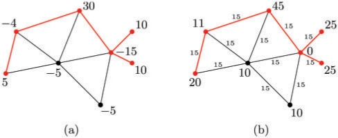
Similar to MWCS, every optimal solution T can be reduced to a tree. Now, let (G,w) be an instance of MWCS with positive and negative vertex weights, and let w′=min_v∈V(G)w_v be its smallest node weight. We construct an instance (G,p,c) of PCST by setting the vertex profits to p(v)=w(v)−w′ for all v∈V and the edge costs to c(e)=−w′ for all e∈E. Clearly, this is a valid PCST instance since all vertex profits and edge costs are positive. Figure 3 illustrates the transformation.

The following theorem justifies that we can concentrate on the transformed instance in order to solve the MWCS problem.

Fig. 3.

Example of an MWCS instance (a) and its transformed PCST counterpart (b). The minimum weight in (a) is −15. Optimal solutions are marked in red color. The MWCS has weight 36, the optimal PCST has profit 126−75=51(=36+15).

THEOREM 1. —

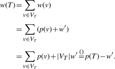
A prize-collecting Steiner tree T in the transformed instance (G,p,c) is a connected subgraph in (G,w) with w(T)=p(T)−w′.

PROOF. —

Obviously, T is a connected subgraph. First, observe that its profit is given by

(4)

since T is a tree. The score of T is

COROLLARY 1. —

A maximum-weight connected subgraph in (G,w) corresponds to an optimal prize-collecting Steiner tree in the transformed instance (G,p,c).

In fact, the two problems are very related. It is not difficult to give also a reduction from PCST to MWCS: we just have to split each edge e∈E and set the weight of the newly created vertex to −c(e). This simple reduction to the NP-complete PCST problem gives an alternative NP-completeness proof for MWCS.

Having reduced the MWCS problem to the PCST problem we briefly summarize the algorithm from Ljubić et al. (2006), which we use to find provably optimal solutions to the MWCS problem. This mathematical programming-based algorithm is currently the fastest way to solve PCST problems to optimality and works very well on the transformed MWCS instances.

Mathematical programming is a powerful tool to address NP-hard combinatorial optimization problems (Nemhauser and Wolsey, 1988). Starting from an ILP formulation modeling the problem under consideration, i.e. a linear program with integer variables, sophisticated techniques like cutting plane methods or Lagrangian relaxation can be combined with branch-and-bound to generate provably optimal solutions. Of course, these methods do not guarantee polynomial-running time in the general case. For many practically relevant instances, however, techniques from mathematical programming work astonishingly well. The advantages over ad hoc heuristic methods are threefold: (i) having provably optimal solutions at hand allows evaluating the quality of a model, e.g. the appropriateness of an objective function. (ii) Methods from mathematical programming guarantee the quality of solutions, i.e. each new feasible solution comes with a maximal distance to an optimal solution. This allows the implementation of a trade-off between running time and solution guarantee. (iii) ILP formulations can be interpreted as polyhedra in high-dimensional space. Mathematical analysis of these objects often leads to new insights into understanding the original problem.

The algorithm from Ljubić et al. (2006) starts by applying a number of preprocessing steps to simplify the input network. Then, it transforms the remaining network into a directed graph by introducing an artificial root vertex r and by splitting each original edge into two directed edges, or arcs, of opposite directions. Arc weights and additional arcs from the root to the nodes in the network are set such that a feasible Steiner arborescence, i.e. a directed tree rooted at r, in which only one arc is incident to r, corresponds to a PCST of equal weight.

The algorithm then works on an ILP built on the transformed directed graph. Each vertex and arc has an associated binary variable modeling its presence or absence in the solution. A number of linear inequalities constrain the solution vector to represent a feasible Steiner arborescence. Besides a degree constraint for the artificial root, a class of constraints ensuring that for each chosen vertex exactly one incoming edge must be chosen as well, the model concentrates on the connectedness of the solution: An exponentially large class of inequalities, the cut constraints, ensure that for every selected vertex, which is separated from r by a cut, there must be an arc crossing this cut.

Due to their large number, cut constraints are not considered at once, but iteratively added to the formulation if violated by the current solution. This technique, combined with a linear programming-based branch-and-bound algorithm, is called branch-and-cut and works particularly well if violated inequalities can be found in polynomial time. Here, this is the case since violated cut constraints can be detected by a maximum-flow algorithm in a support graph with arc-capacities given by the current linear programming solution.

The above algorithm outputs one optimal solution. In practice, users often like to obtain a list of promising solutions for manual inspection. Instead of applying straightforward deletion and re-iteration, we propose a different approach to generate suboptimal solutions: in our ILP approach, binary variables x_v determine the presence of nodes in the optimal subgraph S, that is, x_v=1 if v∈V(S) and x_v=0 otherwise. Now let S be an optimal subnetwork as identified by the branch-and-cut algorithm. Adding the Hamming distance-like inequality

with α∈[0, 1] and re-optimizing leads to a best solution differing in at least α|V(S)| nodes from S. This procedure can be iterated k times. The advantages of this strategy are 2-fold: first, the user can determine the number k of suboptimal solutions that should be reported and, second, he or she may adjust the variety of solutions via the parameter α.

4 RESULTS

4.1 Functional modules in lymphoma network

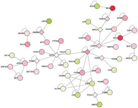
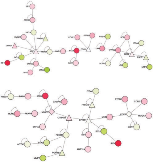
Using our novel approach we identify the optimal-scoring subnetwork (Fig. 4) for the combined score using a restrictive FDR of 0.001. This subnetwork consists of 46 nodes and has a cumulative score of 70.2. The 37 positive-scoring nodes attain a weight of 102.9 and the 9 negatively scoring nodes have a score of −32.8. The theoretical upper bound of the solution in a completely connected graph, given by the cumulative score of all positive nodes, is in this case 145.4. For the given network and under these restrictive conditions our algorithm collects 70.8% of all positive scores. Figure 5 shows the next best solutions with α=0.5.

Fig. 4.

Optimal subnetwork detected using a score based on the P-values of a gene-wise two sided t-test and an univariate Cox regression hazard model. A restrictive threshold equivalent to an FDR of 0.001 was used. The derived subnetwork captures the characteristically differentially expressed-interaction modules associated with the increased malignancy of the ABC subtype. Coloring is according to the fold change where red denotes an over-expression in ABC and green in GCB. Diamond nodes represent negative-scoring genes additionally included in the optimal solution.

Fig. 5.

Examples of suboptimal solutions corresponding to the optimal solution depicted in Figure 4. A Hamming distance of 50% was requested for these solutions. Both subgraphs share 23 nodes with the optimal solution (circles) but also include new ones (triangles). The upper solution achieves a score of 61.5 (87.7%), the lower solution has a score of 52.5 (74.8%) as compared to the optimal solution (70.2). The addition of FGFR1 (first and second suboptimal solution) and GRB2 (first suboptimal solution) within the ‘by-stander cell module’ highlights the biologically relevant interaction between the malignant B-cells and the non-neoplastic network of by-stander cells.

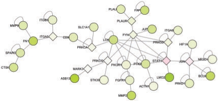
Further we capture interactome modules that have been described to play major biological roles in the GCB and ABC DLBCL subtypes. For example, the proliferation module which is more highly expressed in the ABC DLBCL subtype (Rosenwald et al., 2002) is also evident in our current analysis and includes the genes MYC, CCNE1, CDC2, APEX1, DNTTIP2 and PCNA. Likewise, genes IRF4, TRAF2 and BCL2, which are associated with the potent and oncogenic NFκB pathway, also clustered together as illustrated in Figure 4. Whereas the two previously described interactome modules were derived from genes/proteins expressed in the malignant cells, our algorithm also identified interactome modules (Fig. 6) derived from non-malignant by-stander cells in the lymphoma specimens. In particular, Fibronectin, SPARC, MMP9, CTSK, ITGA5 and ITGB5 showed tight clustering and represent proteins that are expressed in non-malignant fibroblasts and histiocytes (Rosenwald et al., 2002).

Fig. 6.

Optimal subnetwork detected using a score based on the P-values of a one sided t-test for over-expression in GCB and survival as in Figure 4 for an FDR of 0.05.

4.2 Validation

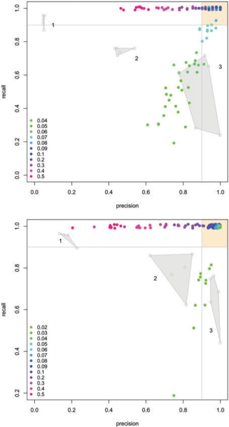
To validate the performance of our approach including the scoring function and search algorithm we simulated an artificial module according to Rajagopalan and Agarwal (2005). Based on the topology of our lymphoma network we selected two subnetworks of biologically relevant sizes (46 and 143) as signal components. Following the proposal of Rajagopalan and Agarwal (2005) we set signal P-values uniformly distributed between 0 and 10⁻³ and background noise P-values uniformly distributed between 0 and 1. Since our approach allows for the finetuning of the signal noise decomposition by the FDR we scan a large range of FDRs and evaluate the obtained solutions in terms of recall (true-positive rate) and precision (ratio of true positives to all positively classified). To assess the variability of the solutions we ran 10 repetitions for each single FDR step. The silhouette of the recall/precision curve, (adapted from Sing et al., 2005) for the module of size 46 includes the optimal solutions with a maximum recall and precision of exactly one (Fig. 7, upper plot). In particular we find a large number of solutions covering the FDR range of 0.7 to 0.3 in the upper right region with a recall and precision higher than 80%. We contrast the performance of our approach to that of Ideker et al. (2002) as implemented in the Cytoscape (Cline et al., 2007; Shannon et al., 2003) plugin jActiveModules. Since their algorithm provides no adjustable scoring function, we follow the proposal of Ideker et al. (2002) and recursively apply their algorithm to the obtained solution three times for five independent simulations. Thus we obtain three discrete solution spaces visualized as shaded polygons representing their convex hulls in Figure 7. Clearly none of these solutions falls within the region of high precision and recall in the upper right corner. Instead one obtains a set of overly large subnetwork constisting of 865 nodes on average, corresponding to 42.5% of the entire network and 18.8 times the size of the hidden signal component. This is reflected by a poor precision of 0.05. After two recursive iterations the number of false positives was reduced substantially and the resultant subnetworks were considerably smaller ranging from 11 to 36 nodes. However, this solution displayed a large variance especially of the recall ranging from 23 to 71%. A similar behavior was observed for the larger module (size 143), see Figure 7, lower plot.

Fig. 7.

Plot of the recall versus precision of a batch of solutions calculated for wide range of FDRs with 10 replications each. For the algorithm by Ideker et al. (2002) we display the convex hulls of solutions obtained by applying their algorithm recursively three times to five independent simulations. We evaluated two different signal component sizes (46, upper plot and 143, lower plot) with the same procedure. Clearly, the presented exact approach captures the signal with high precision and recall over a relatively large range of FDRs. None of the solutions delivered by the heuristic approach falls within the upper right region of high precision and high recall (colored in yellow). For better visualization data points have been jittered in y-direction.

5 DISCUSSION

In the recent years, the integrated analysis of gene expression data in the context of PPI has received considerable attention (Cabusora et al., 2005; Guo et al., 2007; Ideker et al., 2002; Nacu et al., 2007; Rajagopalan and Agarwal, 2005; Sohler et al., 2004). The main objective of these analyses is the derivation of biologically interesting subnetworks of interpretable size from large scale PPI data. This can be expressed as the problem of finding optimal-scoring subgraphs as stated, for the first time, by Ideker et al. (2002). Here we transform the problem to the well-known PCST problem from Operations Research. Thus, we give an alternative NP-completeness proof and, more importantly, we are able to solve large instances of this problem in reasonable computation time to provable optimality by an ILP approach for the transformed problem. Additionally, this allows us to calculate suboptimal solutions with given Hamming distances to previously found solutions. We present an application of our approach using a large PPI network from HPRD (Mishra et al., 2006; Peri et al., 2003) in combination with the comprehensive and well-established microarray dataset from lymphoma patients (Rosenwald et al., 2002). This dataset also provides valuable information of patients’ survival which can be used in a Cox regression hazard model to measure the contribution of each gene to malignancy of the tumor. In contrast to previous studies we do not restrict our analysis to differences in expression between conditions (in our case two lymphoma subtypes) but also include the P-values of the Cox regression into our analysis to derive functional modules that are specifically associated with the different malignant behavior of the tumor subtypes.

In an effective-algorithmic approach, a well-defined objective function is as important as a good search procedure. Therefore we first combine the set of P-values derived from various experiments by an order statistics-based approach to obtain a P-value of P-values as a scalable measure of overall significance. Then we fit a beta-uniform mixture model on the entire set of raw P-values of all nodes in the interaction network. Thus, we achieve a signal-noise decomposition on which we deduce a scoring function of P-values as a likelihood ratio of the signal and noise component. Thus, we deduce a scalable scoring function with a meaningful interpretation of the adjustment parameter as FDR. The additivity of this logarithmic score allows us to effectively formulate and exactly solve the problem of optimal subgraph identification by an ILP approach.

Inspired by the problem of finding local-sequence alignments we strive to identify local maximal-scoring network regions. Given a negative-expectation value of the scoring functions as realized by an appropriate choice of the FDR, we achieve an efficient localization of the resulting region of interest. Our approach makes it possible to fine-tune the size of the resultant subnetworks and thereby ‘zoom’ into the maximal-scoring region of interest in the interaction network.

Our order statistics-based approach to aggregate the P-values from different experiments is equivalent to that adopted by Ideker et al. (2002). However, we explicitly allow the user to require a predefined number of P-values to be significant (e.g. the first, second,…, nth order statistic) instead of only taking the maximum over all order statistics, which is naturally included in our approach. However, asking for the maximum only can lead to serious problems in cases of highly variable signal content among the P-values of different experiments where the highest signal content will dominate the resulting score. As a case in point, analyzing our lymphoma network, the algorithm of Ideker et al. (2002) only yields solution based on the gene expression P-value. Obviously, the biologically important but statistically weaker signal cannot be detected in combination with a more dominant signal by this approach.

To our knowledge, the presented method allows for the first time the exact decomposition of PPI networks into optimal-scoring subnetworks and suboptimal networks of a given dissimilarity as defined by the Hamming distance of the graphs’ node-incidence vectors. In contrast to previously published methods, our algorithm computes provably optimal solutions without computationally demanding parameter optimization usually necessary in heuristic approaches. Furthermore, heuristic methods do not guarantee to find the optimal solution and are unable to assess the solution quality.

As a representative of these heuristic approaches we chose the algorithm of Ideker et al. (2002) as implemented in Cytoscape (Cline et al., 2007; Shannon et al., 2003) and compared the performance to that of our exact approach. The results clearly demonstrate the shortcomings of the heuristic approaches. Since recursive applications of the algorithm are required, only a limited number of isolated solution sizes can be obtained. None of the solutions comes close to the high-accuracy region showing both, high precision and high recall. The high number of true positives in the first run is paid for with an exorbitantly high number of false positives as reflected by the sizes of the results from the initial run. On average 865 nodes were reported for networks with the small signal component of 46 in the first step, corresponding to a true positive (TP)/false positive (FP) ratio of 18.8. A subsequent application of the algorithm yielded on average networks of 75 nodes, 46.4% of which where true positives. Precision can still be improved by a third run but this comes at the expense of recall rates down to 24%. This is an effect of the nestedness of the recursive solutions, where true positives neglected in one step will not be contained in any later solution.

Although Ideker et al. (2002) claim that many high-scoring subnetworks highlight biologically interesting regions although not being optimal in the sense of the objective function it must be kept in mind that the solutions provided by their algorithm are quite variable and heavily dependent on the choice of the parameter settings (seed, number of iterations and annealing temperature). More importantly, the scoring system of Ideker et al. (2002) and those related to it lack an explicit signal/noise decomposition and thus provide no estimation about the size of the signal content. This can pose a serious obstacle for these approaches in the case of low-signal content or the even worse scenario of random noise only. Applying batches of P-values randomly drawn from a uniform(0,1) distribution to our network the implementation of Ideker et al. (2002) still reports solutions of 770 nodes (37% of the entire network) on average with scores within the same range as those of containing the signal modules. Subsetting these solutions by reapplying the algorithm still yields networks of sizes between 130 and 210 nodes. Obviously a major drawback of these scoring systems is that due to the lacking estimate of the signal content prior to the search phase no distinction between a true-signal component and a ‘best noise’ aggregate can be made. This problem is solved by the integrated signal-noise decomposition based on a beta-uniform mixture model of our approach. In fact all tests with random P-values as input yielded a fitted model with a mixture parameter λ of 1 corresponding to a signal content of 0. Consistent with that we obtain a parameter a=1 of the signal beta distribution and consequently a score of zero for all nodes (Equation 3).

Nevertheless, heuristic approaches may be able to deliver biologically relevant solutions as claimed by Ideker et al. (2002) if the proportion of signal is high enough. Especially in case of low-signal content the biological relevancy of the obtained solution may be questionable, and even after recursive application of the algorithm the quality of the obtained subnetwork is hardly assessable due to the high variability. Inherently, all published heuristic methods based on the approach of Ideker et al. (2002) share one of the discussed drawbacks either in terms of search algorithm or scoring function. Therefore it is highly desirable to attain truly optimal solutions with an explicit estimate of the signal content and control of the FDR as provided by the presented approach.

We emphasize that, despite the underlying computational complexity, our algorithm runs very fast on biologically relevant instance sizes: our software tool heinz computes provably optimal results usually in a few minutes; profiling our implementation we measured a median runtime of 182 seconds for test runs on 1000 score-permuted graphs. Most importantly we demonstrate that our approach discovers biologically meaningful modules in a lymphoma interaction network which include and extend the results reported by Rosenwald et al. (2002) which have been described to be of importance in the pathogenesis of the GCB and ABC DLBCL subtypes. In general, the integration of survival and expression data into the analysis of PPI networks exhibits perturbed interaction modules associated with the malignancy of the tumor and can yield new insights into tumor biology on a cellular level.

In the future, we plan to generalize our method to an even broader application setting. As a first step, we propose to integrate edge weights, which could, for example, be derived from correlation of gene expression as used by Guo et al. (2007) or from P-values of interaction predictions with STRING (von Mering et al., 2007). Furthermore, we intend to provide an interface to non-commercial optimization libraries and to integrate our algorithm into the Bioconductor environment (Gentleman et al., 2004).

REFERENCES

- Aittokallio T, Schwikowski B. Graph-based methods for analysing networks in cell biology. Brief. Bioinform. 2006;7:243–255. doi: 10.1093/bib/bbl022. [DOI] [PubMed] [Google Scholar]
- Andersen P, Gill R. Cox's regression model for counting processes: a large sample study. Ann. Stat. 1982;10:1100–1120. [Google Scholar]
- Blenk S, et al. Germinal center B cell-like (GCB) and activated B cell-like (ABC) type of diffuse large B cell lymphoma (DLBCL): analysis of molecular predictors, signatures, cell cycle state and patient survival. Cancer Inform. 2007;3:409–430. [PMC free article] [PubMed] [Google Scholar]
- Byrd RH, et al. A limited memory algorithm for bound constrained optimization. SIAM J. Sci. Comput. 1995;16:1190–1208. [Google Scholar]
- Cabusora L, et al. Differential network expression during drug and stress response. Bioinformatics. 2005;21:2898–2905. doi: 10.1093/bioinformatics/bti440. [DOI] [PubMed] [Google Scholar]
- Carey VJ, et al. Network structures and algorithms in Bioconductor. Bioinformatics. 2005;21:135–136. doi: 10.1093/bioinformatics/bth458. [DOI] [PubMed] [Google Scholar]
- Cline MS, et al. Integration of biological networks and gene expression data using Cytoscape. Nat. Protoc. 2007;2:2366–2382. doi: 10.1038/nprot.2007.324. [DOI] [PMC free article] [PubMed] [Google Scholar]
- Fisher RA. Combining independent tests of significance. Am. Stat. 1948;2:30. [Google Scholar]
- Flannick J, et al. Graemlin: general and robust alignment of multiple large interaction networks. Genome Res. 2006;16:1169–1181. doi: 10.1101/gr.5235706. [DOI] [PMC free article] [PubMed] [Google Scholar]
- Friedman N. Inferring cellular networks using probabilistic graphical models. Science. 2004;303:799–805. doi: 10.1126/science.1094068. [DOI] [PubMed] [Google Scholar]
- Gentleman RC, et al. Bioconductor: open software development for computational biology and bioinformatics. Genome Biol. 2004;5:R80. doi: 10.1186/gb-2004-5-10-r80. [DOI] [PMC free article] [PubMed] [Google Scholar]
- Guo Z, et al. Edge-based scoring and searching method for identifying condition-responsive protein-protein interaction sub-network. Bioinformatics. 2007;23:2121–2128. doi: 10.1093/bioinformatics/btm294. [DOI] [PubMed] [Google Scholar]
- Ideker T, et al. Discovering regulatory and signalling circuits in molecular interaction networks. Bioinformatics. 2002;18(Suppl. 1):S233–S240. doi: 10.1093/bioinformatics/18.suppl_1.s233. [DOI] [PubMed] [Google Scholar]
- Kelley BP, et al. Conserved pathways within bacteria and yeast as revealed by global protein network alignment. Proc. Natl. Acad. Sci. USA. 2003;100:11394–11399. doi: 10.1073/pnas.1534710100. [DOI] [PMC free article] [PubMed] [Google Scholar]
- Lindgren W. Statistical Theory. New York: Chapman & Hall; 1993. [Google Scholar]
- Ljubić I, et al. An algorithmic framework for the exact solution of the prize-collecting steiner tree problem. Math. Program. Ser. B. 2006;105:427–449. [Google Scholar]
- Mishra GR, et al. Human protein reference database–2006 update. Nucleic Acids Res. 2006;34(Database issue):D411–D414. doi: 10.1093/nar/gkj141. [DOI] [PMC free article] [PubMed] [Google Scholar]
- Nacu S, et al. Gene expression network analysis and applications to immunology. Bioinformatics. 2007;23:850–858. doi: 10.1093/bioinformatics/btm019. [DOI] [PubMed] [Google Scholar]
- Nemhauser G, Wolsey L. Integer and Combinatorial Optimization. New York, USA: John Wiley & Sons; 1988. [Google Scholar]
- Peri S, et al. Development of human protein reference database as an initial platform for approaching systems biology in humans. Genome Res. 2003;13:2363–2671. doi: 10.1101/gr.1680803. [DOI] [PMC free article] [PubMed] [Google Scholar]
- Pounds S, Morris SW. Estimating the occurrence of false positives and false negatives in microarray studies by approximating and partitioning the empirical distribution of p-values. Bioinformatics. 2003;19:1236–1242. doi: 10.1093/bioinformatics/btg148. [DOI] [PubMed] [Google Scholar]
- R Development Core Team. R: A Language and Environment for Statistical Computing. Vienna, Austria: R Foundation for Statistical Computing; 2006. [Google Scholar]
- Rajagopalan D, Agarwal P. Inferring pathways from gene lists using a literature-derived network of biological relationships. Bioinformatics. 2005;21:788–793. doi: 10.1093/bioinformatics/bti069. [DOI] [PubMed] [Google Scholar]
- Rosenwald A, et al. The use of molecular profiling to predict survival after chemotherapy for diffuse large-B-cell lymphoma. N. Engl. J. Med. 2002;346:1937–1947. doi: 10.1056/NEJMoa012914. [DOI] [PubMed] [Google Scholar]
- Shannon P, et al. Cytoscape: a software environment for integrated models of biomolecular interaction networks. Genome Res. 2003;13:2498–2504. doi: 10.1101/gr.1239303. [DOI] [PMC free article] [PubMed] [Google Scholar]
- Sharan R, Ideker T. Modeling cellular machinery through biological network comparison. Nat. Biotechno. 2006;24:427–433. doi: 10.1038/nbt1196. [DOI] [PubMed] [Google Scholar]
- Sing T, et al. ROCR: visualizing classifier performance in R. Bioinformatics. 2005;21:3940–3941. doi: 10.1093/bioinformatics/bti623. [DOI] [PubMed] [Google Scholar]
- Smyth GK. Linear models and empirical Bayes methods for assessing differential expression in microarray experiments. Stat. Appl. Genet. Mol. Biol. 2004;3 doi: 10.2202/1544-6115.1027. Article 3. [DOI] [PubMed] [Google Scholar]
- Sohler F, et al. New methods for joint analysis of biological networks and expression data. Bioinformatics. 2004;20:1517–1521. doi: 10.1093/bioinformatics/bth112. [DOI] [PubMed] [Google Scholar]
- Srinivasan BS, et al. Current progress in network research: toward reference networks for key model organisms. Brief Bioinform. 2007;8:318–332. doi: 10.1093/bib/bbm038. [DOI] [PubMed] [Google Scholar]
- Therneau T, et al. Martingale-based residuals for survival models. Biometrika. 1990;77:147. [Google Scholar]
- von Mering C, et al. STRING 7–recent developments in the integration and prediction of protein interactions. Nucleic Acids Res. 2007;35(Database issue):D358–D362. doi: 10.1093/nar/gkl825. [DOI] [PMC free article] [PubMed] [Google Scholar]
- Wasserman LA. All of Statistics: A concise course in statistical inference. 2nd edn. New York, USA: Springer; 2005. [Google Scholar]