Efficient algorithms for accurate hierarchical clustering of huge datasets: tackling the entire protein space

Abstract

Motivation: UPGMA (average linking) is probably the most popular algorithm for hierarchical data clustering, especially in computational biology. However, UPGMA requires the entire dissimilarity matrix in memory. Due to this prohibitive requirement, UPGMA is not scalable to very large datasets.

Application: We present a novel class of memory-constrained UPGMA (MC-UPGMA) algorithms. Given any practical memory size constraint, this framework guarantees the correct clustering solution without explicitly requiring all dissimilarities in memory. The algorithms are general and are applicable to any dataset. We present a data-dependent characterization of hardness and clustering efficiency. The presented concepts are applicable to any agglomerative clustering formulation.

Results: We apply our algorithm to the entire collection of protein sequences, to automatically build a comprehensive evolutionary-driven hierarchy of proteins from sequence alone. The newly created tree captures protein families better than state-of-the-art large-scale methods such as CluSTr, ProtoNet4 or single-linkage clustering. We demonstrate that leveraging the entire mass embodied in all sequence similarities allows to significantly improve on current protein family clusterings which are unable to directly tackle the sheer mass of this data. Furthermore, we argue that non-metric constraints are an inherent complexity of the sequence space and should not be overlooked. The robustness of UPGMA allows significant improvement, especially for multidomain proteins, and for large or divergent families.

Availability: A comprehensive tree built from all UniProt sequence similarities, together with navigation and classification tools will be made available as part of the ProtoNet service. A C++ implementation of the algorithm is available on request.

Contact: lonshy@cs.huji.ac.il

1 INTRODUCTION

1.1 Background

Clustering is a fundamental task in automatic processing of large datasets, in a broad spectrum of applications. It is used to unravel latent natural groupings of data items. Hierarchical clustering methods aim to furthermore categorize data items into a hierarchical set of clusters organized in a tree structure. For instance hierarchical clustering is used for automatic recognition and classification of patterns in digital images, stock prediction, text mining and in computer science theory.

Hierarchical connections are especially evident in the biological domain. Gene Ontology (GO; Ashburner et al., 2000) classifies genes into hierarchies of biological processes and molecular functions. The SCOP, CATH and DALI databases classify protein structures into a hierarchy based on structural similarities (Murzin et al., 1995). The ENZYME commission (EC) nomenclature classifies enzymes into a hierarchy based on biochemical classes. Classical taxonomy classifies organisms into an evolutionary tree structure. Notably, the evolutionary tree process driving sequence divergence, underlies the hierarchical classification of protein families, and make it an especially appealing playground for hierarchical clustering methods. UPGMA (Unweighted Pair Group Method using arithmetic Averages) is arguably the most popular hierarchical clustering algorithm in use to date, especially for gene expression (D'haeseleer, 2005) and for protein sequence clustering (Liu and Rost, 2003).

One of the daunting problems in the field of computational biology is the development of automatic methods for structure and function prediction from protein sequence. This challenge is emphasized by the glut of protein sequences deposited in public databases (Suzek et al., 2007).

ProtoNet (Kaplan et al., 2004, 2005) uses UPGMA to build a hierarchy of protein sequences from sequence similarities. It was shown that this automated procedure is especially useful for prediction of function (Sasson et al., 2006), remote homology (Shachar and Linial, 2004) and structure (Kifer et al., 2005). Since the clustering is unsupervised, it is independent of available knowledge, and can thus automatically unveil clusters of novel biological significance. Other large-scale unsupervised (i.e. using only sequence) methods are Systers (Krause et al., 2005) and CluSTr (Petryszak et al., 2005), which utilize single-linkage clustering to cope with the data size.

1.2 Hierarchical clustering by UPGMA

Hierarchical clustering algorithms construct a hierarchy of input data items. Agglomerative clustering methods create a hierarchy bottom-up, by choosing a pair of clusters to merge at each step. The result is a rooted binary tree. N leaves correspond to input data items (singleton clusters), and N−1 inner nodes (clusters) correspond to groupings in coarser granularities at higher tree levels. Merge scores correspond to dendrogram heights. The hierarchy is often used to infer knowledge from cluster statistics, as well as relatedness at varying granularities.

Agglomerative clustering methods usually take an input of pairwise similarities among data items, from which cluster similarities are then inferred. Different formulations have been used to define pairwise similarities across clusters. Single-linkage methods, use the nearest pair of data points. A careful single-linkage implementation can cluster the whole set, reading one edge at a time (O(1) edges in memory). Hence, single linkage is scalable to large datasets, however it is highly susceptible to outliers since only the minimum edge is considered in each step.

The most commonly used hierarchical clustering formulation is average linkage (Sokal and Michener, 1958) commonly referred to as UPGMA. It uses the mean similarity across all cluster data points and is thus more robust than single-linkage methods. UPGMA is intuitively appealing, and is a particularly practical algorithm owing to the stability of the arithmetic mean. It has been cited extensively, especially in the biological domain (e.g. D'haeseleer, 2005).

UPGMA is a text-book algorithm for correct reconstruction of sequence divergence processes (Durbin et al., 1999). Thus the exact UPGMA solution carries practical implications for understanding of tree processes underlying molecular evolution. Whilst more sophisticated algorithms exist for reconstruction of evolutionary trees, UPGMA 's runtime scales well to input size, and is often the algorithm of choice for the clustering of large sets with comparable performance (Lazareva-Ulitsky et al., 2005).

The problem however, is that UPGMA (or e.g. complete-linkage) requires the entire similarity matrix in memory. Since the number of pairwise relations is asymptotically quadratic in the number of clustered items (O(N²)), the matrix becomes impossibly large to hold in memory even for moderately large datasets. Even for sparse similarity data, as in the case of a BLAST (Altschul et al., 1997) similarities reported here, data is still orders of magnitude too large to hold in memory for UPGMA. Due to rapid accumulation of data (e.g. Table 1), UPGMA is rendered impractical for a variety of tasks.

Table 1.

Size of clustered UniRef90 data, extrapolated future sizes and the appropriate memory requirements

	Memory	|E|
	GB	(No. of edges)
Current – UniRef90 rel. 8.5, June 2006 (N =1.80M)
Raw BLAST similarities (directed multi-graph)	50	2.5×109
Actual sparse similarities (symmetric, undirected)	30	1.5×109
Full non-sparse possible similarities	12 981	1.6×1012
Extrapolated Future – UniRef90 rel. 13.1, March 2008 (N =3.61M)
Actual sparse similarities (symmetric, undirected)	122	6.1×109
Full non-sparse possible similarities	52 262	6.5×1012

Expected memory requirements are based on a conservative estimateof 20 bytes per edge for sparse data, and 8 bytes for full matrices. Extrapolation is based on the actual growth in the number of sequences in UniRef90, when a fixed degree of sparsity is assumed. A strong 32-bit workstation has up to 4 GB of physical memory, which in practice can hold about 40–200 M edges.

Current large-scale methods for sequence clustering cope with the size issue by either single-linkage clustering (Krause et al., 2005; Petryszak et al., 2005), supervised data pre-selection (e.g. Tatusov et al., 1997), or other heuristics. The ProtoNet method (Kaplan et al., 2005) addressed size by using a reduced set of Swiss-Prot sequences (10%) to build a high quality UPGMA tree skeleton, to which the larger TrEMBL set was appended.

Here, we develop a framework for finding the correct UPGMA tree for very large data under any practical memory constraint. The mass of all detectable sequence similarities in the entire set of protein sequences is now directly clusterable. The result is a robust evolutionary-driven tree of nearly 2 million non-redundant sequences. The tree corresponds very well with known protein families.

1.3 Goal

We aim to provide a practical UPGMA algorithm which is not limited by memory requirements but guarantees the correct clustering solution. Non-metric considerations are of special interest, as shown for the case of protein sequence clustering. We thus set out to develop a general clustering framework for any type or size of data (not necessarily metric), while maintaining the relative simplicity of hierarchical clustering.

2 THEORY

2.1 Preliminaries

Agglomerative hierarchical clustering algorithms differ in the choice of cluster dissimilarity objective. For clarity, we refer only to UPGMA (average-linkage) throughout the article. The concepts presented here, however, easily apply to other hierarchical clustering formulations as well.

2.1.1 Problem statement and notation

UPGMA takes an input undirected graph of G=(𝕍,𝔼) and edge weights d, where 𝕍 is the set of data items (vertices), 𝔼⊂𝕍×𝕍 is the edge set, and d :𝔼→ℝ⁺ denotes the actual pairwise dissimilarities. We define N≜|𝕍|.

As clusters are being merged, multiple edges are possible between a pair of non-singleton clusters. These are collated into average edges, and are referred to as ‘thick’ edges throughout this article. Thick edges are cluster-pair unique, and possibly encompass more than one ‘thin’ input edge in the cluster multi-graph. For presentation clarity, we will assume that 𝔼 is symmetric (i.e. d_ij=d_ji) and ignore meaningless self-loops (e_ii). We will think of dissimilarities as distances. Hence lower dissimilarities can be interpreted as ‘closer’ clusters. However, we do not require that dissimilarities are metric distances, by the formal mathematical notion, unless otherwise stated. Moreover, the triangle inequality does not hold for our data (Fig. 1).

Fig. 1.

Illustration of non-metric constraints imposed by BLAST similarities (edges) for three multidomain Swiss-Prot sequences. False transitivity is possible due to CSKP_HUMAN. The missing triangle edge is due to no biological relatedness and no sequence similarity. It violates the triangle inequality since e_jl ≰e_il+e_ij. Triangle-offending missing edges prevent UPGMA from falsely clustering unrelated proteins together, by increasing average cluster dissimilarities.

2.2 Sparse UPGMA

𝔼 is considered sparse if not all possible pairs exist in the input graph (∃i,j∈𝕍:e_ij ∉𝔼). For instance, the sets (𝔼) of all BLAST sequence similarities, or all protein–protein interactions, are sparse.

In this section, we formulate UPGMA for sparse inputs, and give a suitable algorithm—Sparse-UPGMA (Fig. 2). We take advantage, in time and memory complexity, of the data's sparsity, to allow clustering of large sets. It is correct and efficient for non-sparse inputs as well. Based on Sparse-UPGMA, in the next sections we present a novel class of memory-constrained UPGMA (MC-UPGMA) algorithms which do not require all edges in memory at once.

Fig. 2.

Sparse UPGMA. E is typically implemented as a minimum heap data structure, extended with logarithmic time removal of non-minimum elements. The output tree and cluster heights are given by e_ijs. The algorithm is correct for non-sparse inputs as well.

2.2.1 Missing edges

In UPGMA the arithmetic mean is used to measure distance across clusters.

(1)

Equation (1) (or any other average-linkage formulation) is not well defined for sparse inputs (i.e. when e_pq ∉𝔼). To expand d's domain to all vertex pairs (i.e. now d :𝕍×𝕍→ℝ⁺), we override the previous notation to introduce a missing value completion rule.

Where input d_ij's are used when available and ψ is used otherwise. Hence, ψ is a detection threshold used to account for missing edges in the average distance across two partially connected clusters. It does not imply that all clusters are connected; rather, it is used only for missing value completion across connected clusters. Throughout this work, e_ij's are replaced with d_ij in Equation (1) to denote the actual average dissimilarity.

2.2.2 Leveraging sparsity

For suitable inputs, a sparse representation for 𝔼 decreases the memory requirement considerably. Furthermore, new thick edges can efficiently be computed recursively (in O(1)). This calculation, denoted as hereby, requires ψ, cluster sizes |C_*|, and two precalculated edges. For UPGMA we have:

(2)

A similar O(1) expression is easily derived and plugged into our algorithms for other (non-UPGMA) formulations (e.g. for the geometric mean).

2.2.3 Complexity and scalability

Using a suitable binary heap data structure for maintaining 𝔼 sorted, Sparse-UPGMA requires O(ElgV)-time and O(E)-memory, instead of the straightforward O(V³)-time and O(V²)-memory algorithm. These improvements allow for clustering of considerably large sparse datasets. For instance, it can cluster the sparse 75K×75K set of mouse cDNA measurements, that could not be hierarchically clustered in the supplementary data of Frey and Dueck (2007). We were also able to cluster the ProtoNet4 data (114K) requiring time (3 min on a 2.80 GHz machine) that was negligible as compared to the similarity computation preprocessing time. However, this algorithm could not cope with huge datasets, where an O(E) memory requirement is intolerable (e.g. Table 1). Due to poor locality of reference, this algorithm is rendered impractical when the virtual memory demand exceeds the physically available memory.

2.3 Exact (correct) clustering

We define a (UPGMA) clustering solution as exact (or correct), if the order of merges is correct (up to equidistant merges), i.e. it always yields the same solution as UPGMA (or Sparse-UPGMA for sparse inputs), regardless of computational limitations such as memory requirements.

2.4 Multi-Round MC-UPGMA

2.4.1 Outline

We introduce the concept of MC-UPGMA. The proposed solution, breaks the clustering process into multiple rounds. Two computation units carry out each round (Fig. 3). A memory constrained clusterer, holding only a subset of 𝔼 that fits in memory, outputs successive parts of the overall hierarchy. The second unit, the merger (Fig. 3), is a modular unit, external to the clustering, but memory constrained as well. It processes the partial clustering and the set of current edges, to produce valid edges. Edges grow thicker as clusters grow larger. The current set of valid thick edges is input for the clusterer and is used to resume clustering in the successive round.

Fig. 3.

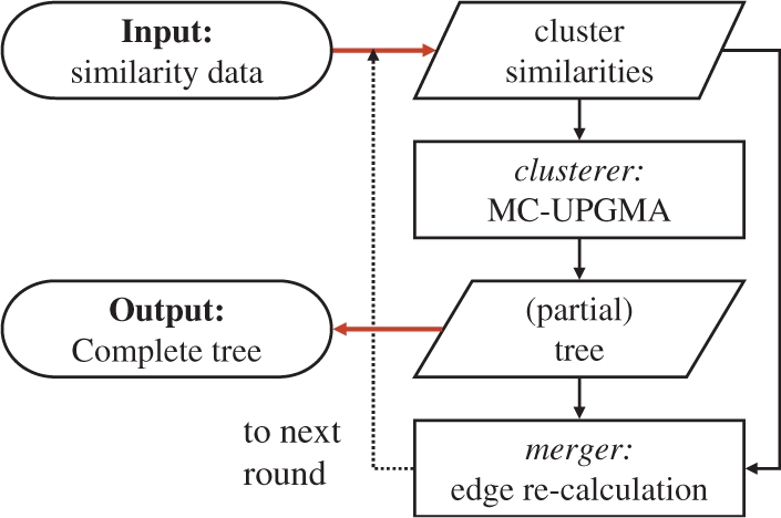
Multi-round MC-UPGMA scheme.

2.4.2 Memory-constrained clustering

Round t of clustering starts from an input (sparse) set of edges, 𝔼^t, between valid (unmerged) clusters. Initially, 𝔼⁰≜𝔼. Clustering is governed by a fixed memory budget parameter M, denoting the maximal number of maintained edges (based on memory size). At initialization, the clusterer loads only the best (minimal) M edges denoted by . Higher Ms may require fewer rounds (due to additional progress per round). We also define

2.4.3 Incorrect naive clustering

At first, it is compelling to naively cluster all loaded edges. We give a simple counter example which will create a wrong tree when this is done. The intention is to motivate construction of a proper stop criterion thereafter.

Assume λ=10 and ψ=100. Let C_i and C_j be merged to some C_k =C_i∪C_j at height d_ij=1. Let d_il = 2, and d_jl≥λ (a non-loaded edge). Suppose C_k is merged with some C_r ≠C_l at height d_kr =7. Then, C_r may not have been the closest neighbor, if e.g. d_jl=10 (since 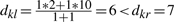). On the other hand, if C_k and C_l are indeed merged, then set d_il=ψ=100 and thus merging is still incorrect ().

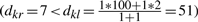Hence, a correct clusterer should be mindful of unseen edges (≥λ), effecting clustering before λ. Such examples are rather prevalent in non-metric datasets. Figure 1 portrays the relevance of this example for the case of clustering sequence similarities.

2.4.4 Uncertain edge intervals

To prevent false clustering of a non-minimal edge, we maintain suitable bounds per edge. The value of d_ij is lower (l_ij) and upper (u_ij) bounded as follows:

It follows that l_ij≤d_ij≤u_ij (for clarity, round indices are omitted hereafter). Hence, maintained edges e_ij are now represented as uncertainty intervals [l_ij,u_ij], rather than by exact d_ij values. The exact value of d_ij is not known to the clusterer unless u_ij=l_ij.

2.4.5 Clusterer algorithm

The clustering algorithm (Fig. 4) design is rather similar to Sparse-UPGMA. Now however, the clusterer loads only the M minimal edges in 𝔼^t (which determine λ^t). Edges d_ij are replaced with intervals [l_ij,u_ij] to accomodate uncertain edge values (due to partial edge data at hand). Clustering halts when it is impossible to identify the minimal edge in the entire 𝔼^t, including the edges in , which are unknown to the clusterer.

Fig. 4.

Multi-round MC-UPGMA clustering—the clusterer. This is a modified version of the code for Sparse-UPGMA (Fig. 2).

2.4.6 Stop criterion

A potential merge (e_ij in Fig. 4) may not be provably minimal if (A) a smaller edge may exist outside the clusterer memory scope or (B) the minimal edge may be at hand but could not be determined unequivocally (as in the given counter example). Since unseen edges are ≥λ, requiring that a merged edge e_ij satisfies u_ij≤λ assures that situation (A) never happens. The latter case (B) manifests itself as edge interval clashes. To assure that d_ij is provably minimal, we consider its interval.

Clustering proceeds while a distinctly minimal edge is at hand—an edge whose upper bound u_ij is below the lower bound of any other edge in (i.e. ∃e_ij ∈E :∀e_rs ∈E :u_ij ≤l_rs; Fig. 4). By maintaining the criterion u_ij≥l_rs in the case where (i, j)=(r,s) we assert that the output merge values d_ij are exact. If only correct merge order, but not exact merge values is required, this criterion can be relaxed to apply only when (i, j) ≠(r,s). In order to construct a full dendrogram (with heights) for the studied proteins, we have used the harsher criterion throughout our analysis.

2.4.7 Correctness and progress

The clusterer always progresses, since after initialization all edges are exact and ≤λ. Furthermore, progress is optimal for this setting, since we have shown a counter example that falsifies the algorithm if it does not halt. Therefore, the number of clusters is reduced in each round, and |𝔼^t+1| is accordingly reduced at a quadratic rate. Once all edges fit in memory (|𝔼^T|≤M), all edge intervals become exact, and Multi-Round MC-UPGMA reduces to Sparse-UPGMA. The clusterer maintains the loop invariant that e_ij is minimal over all edges, if the stop criterion has not been met. Combined with the fact that the clusterer always makes some progress, we conclude that the correct tree is output.

2.4.8 Progress guarantee—metric setting

If the data obeys the triangle inequality, then further clustering progress can be made in each round. The clustering is guaranteed to progress well in this metric setting, so that the tree is complete within only very few rounds. We provide a short claim that shows how good progress can be provably guaranteed for the first iterations. We aim to show how constraints implied from metric considerations render the clustering easier. With some technical rigor, it is possible to generalize this claim.

METRIC PROGRESS LEMMA —

If input edges satisfy the triangle inequality, than Multi-Round MC-UPGMA clusters all edges

PROOF. —

Exact minimal edges do not halt clustering. We will show that inexact edges appear only after . Let be an inexact edge appearing along the clustering process, and assume w.l.o.g. that C_k was created before C_l is merged. Let C_i and C_j be the clusters merged to create C_k, i.e. C_k =C_i∪C_j. Either d_il≤λ or d_jl≤λ, otherwise . Assume w.l.o.g. that only d_il≤λ (i.e. d_jl ≰≤λ), since otherwise e_kl would not have been inexact. From merge order, we have d_ij≤d_il≤λ. Now, note that , otherwise implying (due to the triangle inequality), contradicting our assumption. Plugging in Equation (2), we have . ▪

The progress guarantee is given on the height axis of the forming tree. This translates to very good progress when the data is exponentially distributed (i.e. edges are orders of magnitude different). For instance, this is the case for BLAST similarity E-values. Note that the triangle inequality assumption is never used explicitly by the algorithm, but only to characterize its worst-case progress—the algorithm is correct regardless. Furthermore, if the triangle inequality is used explicitly in Multi-Round MC-UPGMA, the rather crude global ψ bound can be replaced with an edge dependent bound (using the triangle), to reduce clashes and allow further clustering per round. From our experiments (data not shown), the metric assumption can sustain some (bounded) noise, and still yield good progress, i.e. if e_ij≤(1+ɛ)(e_ik+e_kj) is satisfied for some fixed ɛ>0.

2.5 External edge merging

Due to space limitations, we discuss external edge merging very briefly. We then quickly turn to a clustering algorithm which does not need it in the next section.

The merger unit collates edges of newly merged clusters, into thicker edges between the respective parents in the forming tree (as in LOADEDGES, Fig. 5). Merging requires the previous set of edges 𝔼^t−1 and the forming tree. A naive algorithm will form 𝔼^t in memory, thus invalidating the memory constraint. If edges were read in the correct order, however, it is possible to collate one thick edge at a time in memory. This is achieved by appropriate on-disk sorting of only modified edges in 𝔼^t ∖𝔼^t−1. Sorting may be prohibitedly slow when more than a few rounds are required however. The two ideas can be combined to do some limited merging in memory. Notably, merging can be distributed to any number of parallel merging processes. It requires that all edges composing a single thick edge be delivered to the same merging process. This is achieved by mapping edges to processes based on a hash function that is mindful of the current cluster indices to which edges belong.

Fig. 5.

Illustration of Multi-Round MC-UPGMA. FINDANCESTOR uses a suitable data structure for disjoint sets to allow efficient parent look-up. LOOKAHEAD peeks at unloaded edges on disk, and loads only components of currently maintained edges. Afterwards, uncertain edges can be inferred as definitively missing. See text for definition of and ⊕ notations.

2.6 Single-Round MC-UPGMA

2.6.1 Motivation

Up until now, MC-UPGMA built the clustering tree round by round. Although this yielded a practical solution, most of the computation time is spent on preprocessing for the next round of clustering. We address this issue by devising a MC-UPGMA scheme that clusters the entire dataset in a single round.

2.6.2 Approach

Here we aim to combine ideas from the algorithms for external computation of valid edges, together with the idea of careful clustering with λ-missing edges and uncertainty intervals. Clearly, when Multi-Round MC-UPGMAhalts, it is not using its entire memory budget M, since each merge reduces the number of edges in memory. The newly formulated hybrid algorithm presented in this section, will use the freed-up memory to load fresh edges (up to M edges in total) from disk. This reloading enables the clustering to proceed. We assume that input edges are sorted on-disk, and are loaded in order of ascending d_ij values.

An immediate difficulty for reading edges after doing some clustering is imposed by reading ‘old’ invalid edges—those involving clusters which have already been merged. The Single-Round MC-UPGMA algorithm addresses this difficulty. To accommodate edge reading after some clustering has been done, we introduce a new edge representation, that is invariant to the ongoing merging process.

Rereading more edges allows further clustering, where the previous algorithm had to halt. First, once more edges are read, the value of λ increases dynamically and is no longer fixed. Hence, λ-dependent recalculation of l_ijs' reduces interval clashes, and clustering may proceed. Furthermore, uncertain edges resulting from a missing edge can now be updated with certainty to the exact d_ij value, by reading previously missing information, from disk. This capability is due to the introduction of an update procedure for edge intervals.

2.6.3 Edge representation and notation

Let i.e. is now a pair of two quantities; (1) an unnormalized sum of seen singleton (thin) edges and (2) a count parameter, a non-negative integer indicating the number of seen edges accounted for in the sum. We denote the first component as and the second as , corresponding to the numerator and denominator in Equation(2), respectively. We define the ⊕ operator for as the piecewise (dot) plus operator.

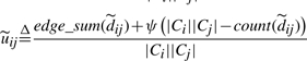
The missing e_il (e_jl), previously replaced with a fixed λ bound, is now dynamically updated with the current λ-value:

(3)

(4)

We think of as a dynamic uncertainty weight. Now, when a missing component of an uncertain edge is read while reloading edges from disk, is incremented. Consequently the respective uncertainty weight diminishes, and the interval tightens up around d_ij. Fully linked edges (i.e. ) become certain (=d_ij). For uncertain edges, missing components of the sum are replaced by the current tightest bound.

Since edges are read in ascending order, λ grows as more edges are loaded. Because uncertain intervals are computed dynamically, lower bounds become tighter as λ grows. Consequently, intervals tighten-up, and edge interval clashes are reduced as more and more edges are loaded. Hence, reloading allows further clustering.

2.6.4 Progress

If the data is metric, the per-round-progress proof shown by the triangle inequality is extended to show that clustering in one round is possible. The reasoning is similar. The triangle inequality guarantees that missing edges are loaded promptly to allow clustering progress. For hard non-metric input, it is theoretically possible that clustering still can not proceed after reloading, while the entire memory budget M is in use. To assure progress, we introduce a look-ahead procedure after which all edges become exact and clustering can effectively resume (Fig. 5).

2.6.5 Complexity

Single-Round MC-UPGMA now requires O(N) (typically N≪M) memory for holding the forming tree. The path compression heuristic allows for efficient cluster look-up.

3 Methods

3.1 Clustered sequence data

We undertake the comprehensive set of all proteins in the UniProt (release 8.1) (Suzek et al., 2007), composed of Swiss-Prot (rel. 50.1) and TrEMBL (rel. 33.1) proteins. UniRef90 (rel. 8.5) non-redundant (<90% identity) sequences were used to represent the protein space. Non-UniRef90 sequences are redundant since they (1) show the same similarity patterns with the rest of the data, thus adding no clustering relevant information and (2) can be regarded as functionally equivalent (Liu and Rost, 2003). The number of sequences affects the volume and especially time for the intensive computation of all-against-all similarities, rather than the clustering.

3.2 BLAST sequence similarities

All sequences in the UniRef90 set were compared using the blastp program of the BLAST (Altschul et al., 1997) 2.2.16 suite, using a E = 100 threshold, low-complexity filtering and default parameters (BLOSUM62, -11,-1). BLAST runs were executed in parallel using a MOSIX grid, as part of the new ProtoNet standard build process.

Sequences were compared using a reciprocal-BLAST-like setting where each sequence is used both as query and database entry. The result is a directed multigraph. It is then transformed to an undirected graph (symmetric dissimilarities) by keeping only e_ij =min(e_ij,e_ji) for i<j, i.e. half of the now-triangular all-against-all sparse dissimilarity matrix. The data sizes before and after this processing are shown in Table 1. Relying on the high capacity of our novel algorithm for very large edge sets, we allow a very permissive threshold (E = 100). This allows for more edges to guide the clustering process, especially for the cases of barely detectable similarities. We rely on UPGMA's robustness to filter out noise manifested as spurious non-significant edges, or amplify weak but consistent similarities by averaging over large clusters. For the case of single-linkage clustering (which is part of our comparative evaluation), including low-significance edges does not interfere with performance either, since they are used only after more significant edges are utilized.

3.3 Protein family keywords

To evaluate the quality of a clustering solution, we measure the correspondence of a tree to external expert classifications of protein families. Here, we use the InterPro (rel 12.1) (Mulder et al., 2007) classification of protein families as a mapping of keywords to protein sequences. InterPro is a consortium of protein families derived from member databases of protein sequence signatures such as Pfam (Finn et al., 2006). InterPro further categorizes keywords into (1) InterPro domains which appear in the context of at least two different non-overlapping protein signatures, and are thus considered a modular protein fragment (positional) and (2) Protein families which refer to a group of proteins in a match set (whole proteins, rather than a sub-region). For this study we have used keywords which incident on at least 2 (10) UniRef90 proteins, with a total of 3752 (3528 are ≥10) InterPro domains, and 8965 (7047) families.

3.4 Performance metrics

A single protein might be associated with multiple keywords, e.g. as in the case of multi-hetero-domains. In the context of a particular keyword k (e.g. InterPro accession IPR001267—thymidine kinase) and the cluster C_i, a protein in C_i is regarded as a true positive (TP) if it has the particular keyword, and as a false positive (FP) if it has a keyword, but it does not have k. Classified proteins outside the cluster, having or not having the particular keywords, are regarded as false and true negatives (FN and TN), respectively. Proteins having no keywords participate in the clustering, but do not affect the evaluation.

A cluster is assigned three quality measures. Specificity () and sensitivity () measure the accuracy of a cluster with respect to cluster members or the reference keyword, respectively. Tree leaves (root), contain a single (all) protein(s), and therefore trivially have full specificity (sensitivity). However, neither convey interesting groupings. A clustering captures a protein family keyword k well, if it contains a cluster having both high specificity and sensitivity for k. This is captured by assigning each cluster-keyword pair a correspondence-score which accounts for both specificity and sensitivity.

(5)

This set-theoretic inspired score (Jaccard score) is a standard clustering performance metric (Kaplan et al., 2005; Krause et al., 2005). The value of 𝒥 ranges from 0 for no correspondence (intersection), to 1 for full agreement when specificity=sensitivity=1. Since 𝒥 ≤specficity and 𝒥 ≤sensitivity, it is a harsh performance metric.

3.5 Best cluster

To evaluate the tree with respect to a particular keyword k, we select the corresponding best cluster. For keyword k, this policy is reflected by taking

(6)

Singleton clusters are omitted, since they do not convey information about classification or clustering quality. By balancing specificity and sensitivity, this score (Equations (5) and (6)) effectively selects against clusters near the root or leaf. This scheme calibrates the groupings (clusters) for the required evolutionary granularity, and selects against intermediate clusters—partial groupings which are artifacts of clustering into a binary tree. It selects biologically meaningful clusters, e.g. with respect to protein family size. To evaluate the tree with respect to a set of keywords K (e.g. InterPro domains) , we select the best cluster per keyword [Equation (6)], and average across K using either equal weights (family-centric) or denote by 𝒥^w a family-size-weighted average (protein-centric).

3.6 Comparison with other methods

To evaluate the contribution of the newly formulated UPMGA tree of all protein sequences, we compare it with trees resulting from other methodologies. We aim to assess the contribution of our work on very large datasets, rather than to assess various clustering methods. We test the clustering performance for different sequence databases, reflecting different difficulty levels and data sizes. We compare MC-UPGMA with three other methodologies which could be applied to this size of data.

3.6.1 CluSTr slim

(Petryszak et al., 2005)—contains the CluSTr pruned tree, downloaded from the EBI ftp. CluSTr uses an in-house single-linkage clustering algorithm, applied to pairwise similarities derived from Smith–Waterman alignments of UniProt (rel. 12.5) and genomic sequences. ClusTR applies a significantly more conservative similarity threshold of E =1e−40 than we (E =100). CluSTr Slim is a pruned tree of clusters ≤1000 with <90% cluster overlap, which maintains CluSTr's predictive power (Petryszak et al., 2005). Removal of proteins in isolated clusters (not in the hierarchy) or the root cluster did not alter results significantly.

3.6.2 Single-linkage clustering

controls for the effects of different alignment algorithm (BLAST versus Smith–Waterman) and similarity thresholds compared to CluSTr. This method applied an in-house single-linkage implementation to our BLAST similarity data.

3.6.3 ProtoNet4 protocol

uses sparse UPGMA clustering to build a tree skeleton from a reduced-size set of high-quality Swiss-Prot proteins, which are regarded as protein family representatives. Sequences from the much larger UniRef90 set (or TrEMBL), are then appended to the existing skeleton independently, based only on similarities to sequences in the reference skeleton. It can thus be regarded as a representative-based heuristic for clustering of very large sets. Accordingly, this method is unable to capture protein families which are not represented well in the Swiss-Prot skeleton. This method does not use similarities within the larger set, but only the manageable smaller clustered set.

4 RESULTS AND DISCUSSION

Sneath (1957) offered the application of computers to taxonomy. 10 years later and some 40 years ago, Fitch and Margoliash (1967) provided what was probably the first automated evolutionary tree for the largest available family at the time—twenty cytochrome-c sequences. Here we tackle the challenge of accurate clustering of nearly 2 million non-redundant sequences, to build a comprehensive tree which aims to capture the evolutionary processes underlying protein families.

4.1 The complete protein families tree

The process started from 1 801 506 UniRef90 proteins. 1107 (0.06%) proteins are singletons having no BLAST similarities, and do not enter the clustering process. From the clustered set, 1 791 206 proteins (99.5%) are clustered into a single tree.

For the first time, we are able to provide an extensive tree of all UniProt sequences in a suitable evolutionary context. The tree is built from the massive set of all sequence similarities detected by an exhaustive search comparing all non-redundant sequences in the UniRef90 set, and agrees very well with external resources. Multiple nearly identical UniProt sequences may be collapsed into a single UniRef90 representative. Here we analyze the UniRef90 collapsed tree, to avoid redundancy issues due to overrepresented protein families. Since our method is unsupervised, it is not fine-tuned for detection of well-characterized protein families.

4.2 MC-UPGMA maintains performance on hard data

The performance of MC-UPGMA on different sets is summarized in Table 2. Swiss-Prot (220 K) is a relatively easy set for UPGMA as well as for single linkage, and surprisingly the performance relative to InterPro families is quite high. Expanding the analysis to a much larger set (UniRef90) slightly reduced the performance for MC-UPGMA but gravely affected single linkage. This observation suggests that Swiss-Prot does not represent the complexity of the whole sequence space. On the other hand, the performance on the UniRef50 set is surprisingly stable (relative to UniRef90). Considering the significantly increased difficulty of UniRef50, this suggests that the richness of the entire tree is maintained by this set. The improvement of MC-UPGMA over single linkage is even more dramatic for the harder case of InterPro domains. Furthermore, UPGMA demonstrated enhanced capacity for handling large protein families (Table 3 and Figure 6). Single linkage performs poorly for large families and thus performance is deteriorated by family size weighting. The ProtoNet4 protocol performs fairly well for large families, since large families are presumably well represented in the Swiss-Prot skeleton. The improvement is due to enhanced sensitivity (Fig. 6).

Fig. 7.

Illustration of thick edges (grey) connecting clusters (blue), and thin input edges (red and black). A thick edge calculation for a pair of clusters C_i and C_j is demonstrated based on three possible components: known (≤λ) thin edges (black), unknown thin edges (due to the memory constraint) that do exist (red, dashed lines), and possible edges connecting C_i and C_j members but do not exist in the sparse input graph (green). Corresponding components in the calculation are color coded accordingly. It is impossible to distinguish non-existing edges from unknown edges without reading the whole input graph. The cluster graph is broken into two connected components in , as long as d_7,9 is missing.

Table 2.

Clustering performance evaluation based on InterPro keywords

	InterPro Families			InterPro Domains
	𝒥	Spec.	Sens.	𝒥	Spec.	Sens.
UniRef90
MC-UPGMA (current)	0.900	0.965	0.926	0.735	0.895	0.798
CluSTr Slim	0.280	0.934	0.292	0.239	0.881	0.253
Single-linkage	0.808	0.952	0.842	0.566	0.878	0.619
ProtoNet4 protocol	0.795	0.941	0.832	0.669	0.901	0.720
UniRef50
MC-UPGMA (current)	0.881	0.959	0.911	0.717	0.887	0.782
Single-linkage	0.794	0.947	0.830	0.557	0.877	0.608
Swiss-Prot
MC-UPGMA (current)	0.935	0.980	0.952	0.809	0.948	0.842
Single-Linkage	0.911	0.968	0.938	0.747	0.941	0.783
UniProt
CluSTr Slim	0.470	0.955	0.489	0.375	0.889	0.406

UniRef90 (1.8M sequences) reflects non-trivial difficulty (sequence identity <90%). UniRef50 (960K) reflects a hard setting (<50%). Swiss-Prot (220K) reflects a moderately sized high-quality set, with some trivial redundancies. All methods, excluding CluSTr Slim and ProtoNet4, were benchmarked by clustering the respective set alone. CluSTr Slim performance on UniProt (redundant, contains trivial cases) is given for reference. CluSTr slim performance is based on an evaluation based only on UniRef90 representatives, but clustering is based on all UniProtKB proteins.

Table 3.

Average UniRef90 performance, unweighted (𝒥) and weighted by non-redundant protein family size (𝒥^w)

	InterPro Families		InterPro Domains
	𝒥	𝒥w	𝒥	𝒥w
MC-UPGMA (current)	0.900	0.856	0.735	0.654
Single-linkage	0.808	0.598	0.566	0.306
ProtoNet4 protocol	0.795	0.782	0.669	0.618

Fig. 6.

Sensitivity of the best cluster for single-linkage (x-axis) versus MC-UPGMA (y-axis) for large protein families—InterPro domains and families with at least 100 UniRef90 representatives. Diagonal line represents identity (x =y). Points above diagonal correspond to higher sensitivity for MC-UPGMA and vice versa. Average specificities are comparable across this set (MC-UPGMA= 0.90±0.15, single-linkage= 0.88±0.18).

Notably, the 1.54 M clusters provided by CluSTr slim produced significantly lower performance than the 1.17 M single-linkage clusters (tied merges are pooled to non-binary clusters). Single-linkage tree performance suffered only minor performance loss, when the CluSTr SLim pruning protocol was applied (not shown). Hence, the difference in performance does not stem from tree pruning. Furthermore, the CluSTr Slim data contained clusters at a variety of granularities. Thus, it is hard to establish the reason for this discrepancy, considering that the two methods do not use exactly the same data.

4.3 Sparse sequence space—well-connected tree

Only 0.09% of the edges (pairs related by BLAST) exist in the input sequence similarity graph (Table 1). However, 1 497 733 of the tree clusters (83.6%) are fully linked, including 426 360 large clusters with at least 10 members. Hence, the edge distribution in the resulting tree is highly non-random even though a very permissive BLAST cutoff was used. Edges appear in dense clusters corresponding to protein families at different levels of evolutionary granularities. The surprisingly high connectivity of the protein tree emphasizes the potential wealth of information laying in similarity patterns across large families (clusters). This information is overlooked by single-linkage methods, which only use O(N) of the input edges.

4.4 Clustering detects poorly connected families

Out of 10 808 InterPro keywords which cover more than 10 proteins in UniRef90, 8218 are captured very well (𝒥≥0.70). Of the 7992 best clusters for these families, only 2467 are fully linked (i.e. not sparse), 2793 are <50% linked, and 792 clusters are highly divergent and are <10% linked. Yet, all are picked up by our method with high accuracy. This demonstrates the capacity of the method to pick up even highly divergent protein families. The latter are dominated by homologous pairs which are not detectable by even a very permissive BLAST threshold, yet MC-UPGMA is able to pick them up, leveraging transitive similarities in large clusters.

4.5 Analysis of multi-round MC-UPGMA run

The Multi-Round MC-UPGMAalgorithm applied to the UniRef90 set required 200 clustering rounds overall (Table 4). Using a single 4 GB memory 4-CPU workstation, we are able to parallelize external merging, and tolerate multiple clustering rounds to cluster the whole set within about 1–2 days. This is orders of magnitude less than the CPU-time required for preprocessing—computation of all BLAST sequence similarities. Additional speedup is possible using grid-computing. In the first three rounds 76% of the clustering (reducing the edge data by 85%) was done. Although the triangle inequality does not hold even for these first rounds, the algorithm is able to sustain some metric distortion and still progress well. The clustering becomes computationally challenging only in the absence of edges, in otherwise connected clusters. The clustering progress per round is significantly slowed down when the triangle inequality is strongly violated due to non-existent BLAST edges (first encountered after 1.37 M merges out of total 1.8 M). Initial tests indicate that Single-Round MC-UPGMA is able to considerably speed up the process (not shown).

Table 4.

Clustering progress for the hard UniRef90 data

t	No. of	Last merge	|tree|	|Et|	|Et|/|E0|
	merges				(%)
1	679915	6e−69	679 915	5.58e+08	36.77
2	430486	1e−24	1 110 401	3.15e+08	20.77
3	258122	8e−05	1 368 523	2.24e+08	14.78
4	26774	0.004	1 395 297	2.14e+08	14.06
5	39712	0.444	1 435 009	1.89e+08	12.47
6	11534	1.052	1 446 543	1.82e+08	11.98
7	5225	1.474	1 451 768	1.78e+08	11.75
8	5948	2.062	1 457 716	1.75e+08	11.50
9	11011	3.533	1 468 727	1.68e+08	11.03
10	4286	4.277	1 473 013	1.65e+08	10.88

First 10 iterations are shown out of total 200. Here, clustering progress per round is significantly slowed down in advanced iterations (see text).

4.6 Protein sequence space inherently non-metric

We argue that the non-metric considerations are inherent to the protein sequence space, and should not be overlooked due to arising computational difficulties. Some of this difficulty stems from limited detection of highly divergent sequences by sequence alignment, as reflected by the partial connectivity of most protein families. However, non-metric constraints are inherent to the protein sequence space due to the modular nature of protein domains. Domain shuffling events may create mixtures of distinct divergence processes, which could not be captured by a single tree for whole proteins. Yet, incorporating this constraint into the clustering problem—by taking into account missing edges in the average cluster dissimilarity—seems to aid UPGMA avoid the pitfalls of false transitivity, as reflected by local sequence alignment (Fig. 1). This is demonstrated by the significant improvement of UPGMA over single-linkage methods as shown for the case of InterPro protein domains (Table 2). Even when the reduced set of Swiss-Prot proteins is used to partition the much larger UniRef90 set (ProtoNet4 in Table 2), the underrepresented UPGMA skeleton still significantly outperforms single-linkage clustering using the whole data.

4.7 Top levels of tree surprisingly meaningful

Since a significant amount of protein families coincide with poorly connected clusters, we stress that the top levels of the UPGMA cluster tree are biologically meaningful and should not be pruned out. Furthermore, our results show that hidden, remote connections between protein families, some overlooked by state-of-the-art specialist methods (e.g. Profile–Profile comparisons), are picked up at these seemingly uninteresting levels. Averaging across large sets of sequence similarities is able to weed out these faint connections, otherwise below the level of random BLAST hits. Indeed, 710 evolutionary connections between protein families were suggested by a systematic scan for putative evolutionary links in the novel tree, most of them have been previously overlooked (submitted for publication).

REFERENCES

- Altschul SF, et al. Gapped BLAST and PSI-BLAST: a new generation of protein database search programs. Nucleic Acids Res. 1997;25:3389–3402. doi: 10.1093/nar/25.17.3389. [DOI] [PMC free article] [PubMed] [Google Scholar]
- Ashburner M, et al. Gene ontology: tool for the unification of biology. The Gene ontology consortium. Nat. Genet. 2000;25:25–29. doi: 10.1038/75556. [DOI] [PMC free article] [PubMed] [Google Scholar]
- D'haeseleer P. How does gene expression clustering work? Nat. Biotechnol. 2005;23:1499–1501. doi: 10.1038/nbt1205-1499. [DOI] [PubMed] [Google Scholar]
- Durbin R, et al. Biological Sequence Analysis : Probabilistic Models of Proteins and Nucleic Acids. Cambridge, UK: Cambridge University Press; 1999. [Google Scholar]
- Finn R, et al. Pfam: clans, web tools and services. Nucleic Acids Res. 2006;34:D247–D251. doi: 10.1093/nar/gkj149. [DOI] [PMC free article] [PubMed] [Google Scholar]
- Fitch WM, Margoliash E. Construction of phylogenetic trees. Science. 1967;155:279–284. doi: 10.1126/science.155.3760.279. [DOI] [PubMed] [Google Scholar]
- Frey BJ, Dueck D. Clustering by passing messages between data points. Science. 2007;315:972–976. doi: 10.1126/science.1136800. [DOI] [PubMed] [Google Scholar]
- Kaplan N, et al. A functional hierarchical organization of the protein sequence space. BMC Bioinformatics. 2004;5:196. doi: 10.1186/1471-2105-5-196. [DOI] [PMC free article] [PubMed] [Google Scholar]
- Kaplan N, et al. ProtoNet 4.0: a hierarchical classification of one million protein sequences. Nucleic Acids Res. 2005;33((Database issue)):D216–D218. doi: 10.1093/nar/gki007. [DOI] [PMC free article] [PubMed] [Google Scholar]
- Kifer I, et al. Predicting fold novelty based on ProtoNet hierarchical classification. Bioinformatics. 2005;21:1020–1027. doi: 10.1093/bioinformatics/bti135. [DOI] [PubMed] [Google Scholar]
- Krause A, et al. Large scale hierarchical clustering of protein sequences. BMC Bioinformatics. 2005;6:6–15. doi: 10.1186/1471-2105-6-15. [DOI] [PMC free article] [PubMed] [Google Scholar]
- Lazareva-Ulitsky B, et al. On the quality of tree-based protein classification. Bioinformatics. 2005;21:1876–1890. doi: 10.1093/bioinformatics/bti244. [DOI] [PubMed] [Google Scholar]
- Liu J, Rost B . Domains, motifs and clusters in the protein universe. Curr. Opin. Chem. Biol. 2003;7:5–11. doi: 10.1016/s1367-5931(02)00003-0. [DOI] [PubMed] [Google Scholar]
- Mulder NJ, et al. New developments in the interpro database. Nucleic Acids Res. 2007;35(suppl. 1):D224–D228. doi: 10.1093/nar/gkl841. [DOI] [PMC free article] [PubMed] [Google Scholar]
- Murzin AG, et al. SCOP: a structural classification of proteins database for the investigation of sequences and structures. J. Mol. Biol. 1995;247:536–540. doi: 10.1006/jmbi.1995.0159. [DOI] [PubMed] [Google Scholar]
- Petryszak R, et al. The predictive power of the CluSTr database. Bioinformatics. 2005;21:3604–3609. doi: 10.1093/bioinformatics/bti542. [DOI] [PubMed] [Google Scholar]
- Sasson O, et al. Functional annotation prediction: all for one and one for all. Protein Sci. 2006;15:1557–1562. doi: 10.1110/ps.062185706. [DOI] [PMC free article] [PubMed] [Google Scholar]
- Shachar O, Linial M. A robust method to detect structural and functional remote homologues. Proteins. 2004;57:531–538. doi: 10.1002/prot.20235. [DOI] [PubMed] [Google Scholar]
- Sneath PH. The application of computers to taxonomy. J. Gen. Microbiol. 1957;17:201–226. doi: 10.1099/00221287-17-1-201. [DOI] [PubMed] [Google Scholar]
- Sokal RR, Michener CD. A statistical method for evaluating systematic relationships. Univ. Kans. Sci. Bull. 1958;28:1409–1438. [Google Scholar]
- Suzek BE, et al. UniRef: comprehensive and non-redundant UniProt reference clusters. Bioinformatics. 2007;23:1282–1288. doi: 10.1093/bioinformatics/btm098. [DOI] [PubMed] [Google Scholar]
- Tatusov RL, et al. A genomic perspective on protein families. Science. 1997;278:631–637. doi: 10.1126/science.278.5338.631. [DOI] [PubMed] [Google Scholar]