

Abstract
MicroRNA (miRNAs) play essential roles in post-transcriptional gene regulation in animals and plants. Several existing computational approaches have been developed to complement experimental methods in discovery of miRNAs that express restrictively in specific environmental conditions or cell types. These computational methods require a sufficient number of characterized miRNAs as training samples, and rely on genome annotation to reduce the number of predicted putative miRNAs. However, most sequenced genomes have not been well annotated and many of them have a very few experimentally characterized miRNAs. As a result, the existing methods are not effective or even feasible for identifying miRNAs in these genomes.
Aiming at identifying miRNAs from genomes with a few known miRNA and/or little annotation, we propose and develop a novel miRNA prediction method, miRank, based on our new random walks- based ranking algorithm. We first tested our method on Homo sapiens genome; using a very few known human miRNAs as samples, our method achieved a prediction accuracy greater than 95%. We then applied our method to predict 200 miRNAs in Anopheles gambiae, which is the most important vector of malaria in Africa. Our further study showed that 78 out of the 200 putative miRNA precursors encode mature miRNAs that are conserved in at least one other animal species. These conserved putative miRNAs are good candidates for further experimental study to understand malaria infection.
Availability: MiRank is programmed in Matlab on Windows platform. The source code is available upon request.
Contact: zhang@cse.wustl.edu
1 INTRODUCTION
MicroRNAs (miRNAs) are endogenous single-stranded non-coding RNAs of ∼22 nt in length. They are derived from long precursors that fold into hairpin structures (Bartel, 2004; Jones-Rhoades et al., 2006). miRNAs have been shown to play fundamentally important roles in animal and plant development (Bartel, 2004; Jones-Rhoades et al., 2006, in stress response in plants (Bari et al., 2006; Chiou et al., 2006; Jones-Rhoades and Bartel, 2004; Lu et al., 2005; Sunkar and Zhu, 2004; Zhou et al., 2007), and in genetic diseases including various types of cancer (Blenkiron et al., 2007; Chen et al., 2007; He et al., 2007; Hobert, 2007; Ma et al., 2007; Ozen et al., 2008; Pedersen et al., 2007; Tili et al., 2007). In animals, most miRNAs bind to 3′ untranslated regions of their target mRNAs and repress the translation of the targets (Bartel, 2004). In contrast, in plants, most mature miRNAs directly base-pair with complementary sites in the coding regions of target mRNAs, resulting in cleavage or degradation of the targets (Bartel, 2004; Jones-Rhoades et al., 2006).
Identification of novel miRNA genes is an eminent and challenging problem towards the understanding of post-transcriptional gene regulation. Two major strategies for identifying novel miRNAs are experimental cloning and in silico prediction (Bartel, 2004; Berezikov et al., 2006; Jones-Rhoades et al., 2006). In a cloning-based approach, distinct ∼22 nt RNA transcripts were first isolated and then intensively cloned and sequenced. However, these methods are highly biased towards abundantly and/or ubiquitously expressed miRNAs; only abundant miRNA genes can be easily detected (Bartel, 2004; Berezikov et al., 2006; Jones-Rhoades et al., 2006). Note that not all miRNAs are well expressed in many tissues, cell types and developmental stages that have been tested (Bartel, 2004). Some miRNAs are expressed constitutively at low abundance, and some miRNAs have preferential or specific temporal and spatial expression patterns. Computational approaches have been developed to overcome some of the technical difficulties of experimental methods. First, in silico methods have been shown to be efficient for finding miRNAs that are expressed at constitutively low levels or in specific tissues (Bartel, 2004). Further, breakdown products of mRNA transcripts, other endogenous ncRNAs (e.g. tRNAs, rRNAs, nat-siRNAs) as well as exogenous siRNAs comprise a large portion of the non-coding small RNA population isolated from the cytoplasmic total RNA extracts (Bartel 2004; Berezikov et al. 2006; Jones-Rhoades et al. 2006; Lagos-Quintana et al., 2001). To avoid erroneously designation of other non-coding small RNAs and even broken mRNA fragments as novel miRNAs, the secondary structures of flanking genomic sequences of cloned small RNAs are further assessed computationally. Only those small RNA sequences reside on arms of hairpin-structured precursors are likely to be miRNAs. However, due to their short length, cloned small RNAs may match to many genome regions that can potentially fold into hairpin structures which may not be unique to miRNAs. Thus, genome-wide screening of novel miRNA precursors is technically involved.
Based on particular strategies adopted, the existing computational methods for miRNA prediction can be grouped into two categories.
Methods in the first category were developed to find homologous miRNAs in closely related species. In these methods, known miRNA precursors were first folded into typical hairpin structures, local features in the hairpins were extracted, and extreme values of these featured were obtained from all known miRNAs. A filter was then constructed to screen novel hairpinned sequences. Those hairpinned sequences that passed the filter were further analyzed in related species to assess their evolutionary conservation (Berezikov et al., 2005; Bonnet et al., 2004; Grad et al., 2003; Lai et al., 2003). As they were designed for, these conservation-based methods built upon this framework were successful in detecting evolutionarilly conserved miRNAs. In order to further identify distantly homologous miRNAs, a probabilistic co-learning method using a paired hidden Markov model (HMM) was recently developed as a more general miRNA prediction method (Nam et al., 2005). All these methods relied mainly on evolutionary conservation to eliminate a large number of false positive predictions. However, a substantial number of lineage- or species-specific miRNA genes do exist (Fahlgren et al., 2007; Kasschau et al., 2007; Lindow and Krogh, 2005; Molnar et al., 2007; Rajagopalan et al., 2006; Zhang et al., 2006), which escape the detection of a conservation-based approach.
In the second category, supervised classification methods, e.g. Support Vector Machines (SVMs), were adopted to train models based on positive sets of genuine miRNA precursors and negative sets of hairpins obtained from exon regions of protein coding genes (Hertel and Stadler, 2006; Ng and Mishra, 2007; Xue et al., 2005). Thanks to the sequence features extracted from the training examples, such classification models were expected to preform well in predicting novel miRNAs from unseen sequences. However, many sequenced genomes are poorly annotated. Hence, it is difficult to obtain a good set of negative training samples for these methods. Moreover, miRNAs are located in intergenic regions and introns. A major task for miRNA prediction is to distinguish miRNA hairpins from other hairpin structures originated from intergenic or intronic sequences. In summary, classification-based methods are not effective on not well-annotated genomes.
The methods in both categories discussed above all require a non-trivial set of positive samples of known miRNAs. Unfortunately, except well-studied model species such as human and Caenorhabditis elegans, most sequenced genomes have a small number of miRNAs reported. For instance, only 38 miRNAs have been identified in the genome of A.gambiae. This is particularly true for viral genomes for which not many miRNAs have been studied or reported (Stern-Ginossar et al., 2007). Furthermore, the small number of known viral miRNAs rarely share any sequence homology (Stern-Ginossar et al., 2007). Yet, viral miRNAs have been shown to play important roles in the pathology of viral infection by targeting host immune systems (Stern-Ginossar et al., 2007).
In short, the importance of miRNAs in post-transcriptional regulation, the lack of a sufficient number of known miRNAs and poorly annotated genomes collectively call for novel effective computational approaches to miRNA prediction.
In this work, we propose and develop a novel ranking algorithm based on random works to computationally identify novel miRNAs from genomes with a few known miRNAs and with poor annotation. Our algorithm uses very few positive samples, requires no negative sample and does not rely on genome annotation. When applied to human data, our approach was able to identify known miRNAs with a relatively high precision and recall. As an application, we applied our algorithm to predict novel miRNAs in A.gambiae, which is the most important vector of malaria in Africa and one of the most efficient malaria vectors in the world. Our analysis also showed that some of putative miRNAs encode mature miRNAs conserved in other species.
2 PROBLEM FORMULATION
In our study, we cast the problem of miRNA prediction as a problem of information retrieval, in which novel miRNAs are to be retrieved from a pool of candidates by the known miRNAs as query samples. Specifically, we model this information retrieval process as belief propagation on a weighted graph, and develop a new ranking algorithm based on random walks.
For a given species, the known miRNAs, putative candidate miRNAs and their relationship can be modeled by a weighted graph G=〈V, E〉. Each vertex v∈V in G represents a known miRNA precursor or a putative candidate, an edge e∈E⊆V × V captures the relation between two vertices linked by the edge, and the weight w of edge e quantifies the relation. In general, edge weights are determined by pairwise distances. For example, two closely related samples may share an edge with a large weight. The degree of vertex vi is di=∑j wij, i.e. the total weight of all edges that are connected to vi. Note that the graph is fully connected, so that there always exists a path between each pair of nodes in the graph.
We refer the known miRNA precursors as query samples and putative candidates as unknown samples. Consider query samples XQ={xq1, xq2, …, xqn} and unknown samples XU={xu1, xu2, …, xum}, where xqi, xuj,∈ℝd. Our goal is to rank XU with respect to XQ. To achieve this goal, we associate each sample xi with a relevancy value fi, where fi=1 for all query samples and fi∈[0, 1] for all unknown samples. A larger fi value means a higher relevancy of xi with respect to the queries. We then sort the relevancy values of all unknown samples and select the top ranked samples as retrieved samples, which constitute our predicted miRNA precursors. Therefore, the key to the ranking algorithm is to precisely compute the relevancy values of all unknown samples. In this study, we adopted the random walks method for this ranking problem, to be discussed next.
3 METHOD
Query by samples is a paradigm for information retrieval in the information retrieval and machine learning fields. Zhou et al. proposed a manifold ranking method, which ranks the data with respect to the intrinsic manifold structure collectively revealed by the given data (Zhou et al., 2004). Different from their work, our method uses Markov random walks to model a belief propagation process and therefore has a direct physical interpretation.
3.1 Ranking based on random walks
Random walks is a classical stochastic process on a weighted finite state graph, which exploits the structure of the given data probabilistically. In the random walks formulation, each sample is treated as a graph vertex, which corresponds to a state on a Markov chain. The one-step transition probability pij from vertex vi to vertex vj can be defined as
| (1) |
or written in the matrix form
| (2) |
where W=(wij) is the weight matrix, D is a diagonal matrix whose i-th diagonal element is di. To facilitate our discussion, we reorder the vertices in a vector so that the query samples come first, followed by the unknown samples. We then partition the matrix as
| (3) |
where PQQ is an n × n transition matrix among the query states, PQU is an n × m transition matrix from the query states to the unknown states, PUQ is a m × n transition matrix from the unknown states to the query states and PUU is a m × m transition matrix for the unknown states. Correspondingly, we partition the weight matrix W and the degree matrix D as
| (4) |
where O is a matrix with all 0.
In our model, when a random walker transits from vi to vj, it will transmit the current relevancy information of vi to vj. This forms a dynamic process of relevancy information propagation: at each iterative step, a vertex transmits its relevancy information to its neighbors, and simultaneously receives the relevancy information from its neighbors. At the end of the iteration, each vertex updates its relevancy value according to the received information. Note that the query vertices only transmit their relevancy information and will never update their relevancy values. Furthermore, since query samples are more important than the unknown ones, the former are assigned higher weights for their relevancy information in transmission. This suggests the following relevancy updating rule,
| (5) |
where k is the iteration index, and α∈(0, 1) the weight of the relevancy from the unknown samples. In our method, fi is also called the ranking score of sample i, which we use to rank the unknown samples.
The matrix form of () is
| (6) |
By (2), () can be turned into
| (7) |
The convergence of the iterations is guaranteed by the following theorem.
THEOREM 1. —
The sequence
generated by the updating rule of () converges when k approaches infinity.
PROOF. —
For convenience, let
, 𝔻=[0,1]m. Let
,
. Then (7) can be written as
(8) To finish our proof, we introduce a mapping T : 𝔻→𝔻 and the measure d on it as follows:
(9)
(10) where xi is the i-th element of vector X. It is easy to show that (𝔻, d) is a complete metric space.
According to the Contractive Mapping Theorem of Banach (Istratescu, 1981), it is suffice to prove that T(f) is a contractive mapping, which holds if R satisfies
| (11) |
To prove (11), recall that 0 < α < 1, and
| (12) |
where 1n=[1, 1, …, 1]T is an n-dimensional vector with all elements 1. It follows that
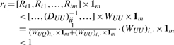 |
(13) |
Therefore, T(f) is a contractive mapping, and (7) converges to a unique fixed point.▪
Therefore, the limit of  and
and  can be substituted by fU, resulting in
| (14) |
which is equivalent to
| (15) |
where I is an m × m identity matrix. Therefore,
| (16) |
3.2 The ranking algorithm
The key to the above discussion and derivation is that we can compute the relevancy values of all unknown states according to (16) without actually performing the procedure of iterative random walks. Therefore, we propose the following ranking algorithm, which runs as follows:
Step 1: Construct graph G=〈V, E〉. For each pair of vertices xi and xj, we introduce an edge between them if they are close to each other.
- Step 2: Measure graph weights W. Here a heat kernel is adopted, i.e. if xi and xj are connected by an edge, the weight of the edge is defined as
where d(·,·) is a distance measure defined on the graph, σ is the heat kernel parameter. Usually, d(i,j) is the Euclidian distance between samples i and j.
Step 3: Compute relevancy values of the samples by solving the matrix problem in equation (16).
Step 4: Rank the samples. Sort the relevancy values of all samples, and select some top ranked samples as the final result.
For the problem of predicting new miRNAs, each sample is represented by a vector of 36 features (Section 3.3), and distance between two samples is the Euclidean distance of the feature vectors. In order to reduce the data noise and computational expense, we make the graph sparse by removing the ‘weak’ edges with low weights.
Since putative miRNAs are to be retrieved by known miRNAs according to the ranking scores of the candidates, we named our miRNA prediction method as miRank.
3.3 Extraction of global and local sequence-structure features
The most salient characteristics of miRNA precursors are their hairpinned secondary structures. In our study, we used RNAfold (Hofacker, 2003) to predict RNA secondary structures. We postulated that the entire hairpin structure of a miRNA precursor could be characterized solely by 36 global and local intrinsic attributes that capture sequence, structural and topological properties of the miRNA precursor.
Four important global features at the structural and topological levels are the normalized minimum free energy of folding (MFE), the normalized base-pairing propensities (number of nucleotides that are paired) of both arms and the normalized loop length. Here the normalization factor is the length of the precursor sequence.
Local features characterize various sequence properties in RNA sequences, which we discuss using an example. As shown in Figure 1, in the hairpin structure from RNAfold (Hofacker, 2003), each nucleotide in the sequence is either paired (indicated by a bracket, ‘(’ or ‘)’) or unpaired (denoted by a dot, ‘.’). The left bracket ‘(’ indicates that a nucleotide is located in the 5′ arm and the paired right bracket ‘)’ means the correspondingly paired nucleotide is in the 3′ arm. No evidence has shown that mature miRNAs have a preference of the 5′ or 3′ arms of their hairpinned precursors. Thus, it is not necessary to distinguish ‘(’ and ‘)’ in the local feature extraction; we use ‘(’ for both situations in the subsequent discussion. For any three adjacent nucleotides, there are eight (23) possible structure configurations: ‘(((’, ‘((.’, ‘(..’, ‘(.(’, ‘.((’, ‘.(.’, ‘..(’ and ‘·s’. We further differentiate each of these eight configurations by the nucleotide—A,C,G,U—in the middle position. Thus, there are 32 (4 × 8) possible sequence-structure configurations for each triplet in the precursors of miRNAs. Similar features have been used in some of the existing methods, e.g. that in Xue et al. (2005).
Fig. 1.

Extraction of local structure-sequence features. (a): the sequence and secondary structure of hsa-mir-20a. (b): the configurations of 32 local sequence-structure features. Frequencies of the 32 features are obtained for each miRNA precursor or putative candidate, and further normalized by the length of the corresponding sequence.
4 EXPERIMENTAL EVALUATIONS AND DISCUSSIONS
4.1 Evaluation of the ranking algorithm on toy examples
In order to show the belief propagation of our new ranking algorithm, along the manifold of the data, we generated a set of toy data, selected one data point as a query sample, and queried the rest samples to rank them.
Figure 2 shows the results on two toy examples, where data are two-dimensional points distributed on X–Y plates. In each of these examples, we chose one point as the query, which is marked by a red plus. The rest points were treated as unlabeled data. In Figure 1, the relevancy values are color coded, i.e. a red indicates a high-relevancy value and a blue indicates a low-relevancy value. It can be seen that the method successfully propagates the query belief to the unknown samples so that the samples that are closer to the query have higher relevancy values.
Fig. 2.

Two toy examples of information propagation using the Markov random walks algorithm. Each dot represents a two-dimensional point distributed on an X-Y plate. In each figure, the dot marked by a red plus is the query. (See online version for the color figure).
4.2 Datasets for miRNA prediction
All reported miRNAs precursor sequences of H.sapiens and A.gambiae (533 and 38, respectively) were downloaded from the miRBase (http://microrna.sanger.ac.uk/sequences/) (Griffiths-Jones et al., 2006) as of September 1, 2007. Genome sequences of H.sapiens and A.gambiae were retrieved from UCSC Genome Browser (http://genome.ucsc.edu/).
For the H.sapiens genome, we randomly extracted non-overlapping fragments of 90 nt from the genome so that no information of genome annotation was used. We first discarded all fragments overlapping with known miRNA precursors. For a fragment not overlapping with any known H.sapiens miRNA precursor, we further predicted its secondary structure using RNAfold (Hofacker, 2003). Nevertheless, not every such fragment would be kept for further analysis. The criteria for retaining hairpinned fragments are as follows: minimum 18 base pairings on the stem of the hairpin structure, maximum -12 kcal/mol free energy of the secondary structure and no multiple loops. The threshold 18 is the lowest number of base pairings, and the threshold -12 is the highest free energy among all genuine animal miRNA precursors. Finally, 1000 of such fragments were arbitrarily chosen and pooled together with some of the known human miRNA precursors—which were all known human miRNA precursors except the ones used as query samples in our experiments—to form the pool of candidates to be ranked by the miRank algorithm. The reason we added those known human miRNA precursors to this pool of samples is to evaluate the prediction performance of the miRank algorithm.
Every chromosome of A.gambiae was fragmented, from 5′-end to 3′-end, using a sliding window of 90 nt and a shift increment of 45 nt. These fragments were folded using RNAfold (Hofacker, 2003), and hairpinned fragments were selected by the same criteria described above. The chosen hairpin sequences formed the initial candidate pool. In the fragmentation, some putative candidates might be cut into two pieces, and have lost their hairpin structures, hence were excluded from the candidate pool. To avoid this, we further fragmented, with the same sliding window and increment, the sequences between each pair of hairpinned fragments next to each other. The secondary structures of the new set of fragments were predicted and selected by the same tool and criteria. This process was iterated until no hairpinned fragment could be found. We obtained 22 297 hairpinned sequences, which included all 38 known miRNAs precursors for A.gambiae.
4.3 Evaluation on human miRNAs
We first evaluated the performance of our miRank algorithm on H.sapiens data based on the known miRNA precursors embedded in the pool of samples to be ranked (Section 4.2). The prediction quality was assessed by the recall and the precision, which are, respectively, defined as:
| (17) |
| (18) |
where TP, FP and FN are numbers of true positive predictions, false positive predictions and false negative predictions, respectively.
The number of query samples is the most critical parameter for algorithm miRank. We tested on H. sapiens data with 1, 5, 10, 15, 20 and 50 known miRNA precursors randomly chosen as query samples. To reiterate, in each of these experiments, the rest known miRNA precursors were combined with the 1000 hairpin sequences extracted from the genome to form the pool of candidates to be ranked (Section 4.2). In each experiment, we chose n topmost ranked candidates, and determined the precision and recall of the result by comparing the chosen candidates with the known human miRNAs that were hidden in the candidate pool. By varying the number n, we obtained the receiver operating characteristic (ROC) curves (Spackman, 1989) for the performance of miRank using different number of query samples, as shown in Figure 3.
Fig. 3.

Precision-recall curves obtained by setting different number of queries. All experiments were performed on human data. The curves from right to left show the results of experiments with query number equal to 1, 5, 10, 15, 20, 50 (See online version for the color figure).
In the extreme case of querying with only one sample, we obtained a precision greater than 70% in the 20 topmost retrieved samples. When we queried with more than 20 query samples, we obtained a high precision of over 95% in the 160 top ranked samples. These results suggest that we can expect miRank to be effective in predicting miRNAs on a species with a small number of reported miRNAs and a poorly annotated genome. Note that the precisions in these experiments could be under-estimated because genuine but unvalidated miRNA precursors may actually exist in the 1000 human hairpinned sequences that were analyzed in the experiment.
Candidates with higher ranks are most likely to be true miRNAs; they are excellent candidates for further experimental validation. To obtain as many putative miRNAs with high confidence as possible, we need to set a ranking score cutoff. Figure 4 shows the prediction precisions with respect to ranking score cutoffs in each of these six experiments. Evidently, each curve in Figure 4 has an inflection point. The precise inflection points in Figure 4 can be obtained by second-order differential. Notably, in the experiments with more query samples, the ranking scores of unknown sample tend to be higher, and prediction precisions by setting the scores at the inflection points as cutoffs are also improved. For each experiment, the score at the inflection point can be a reasonable cutoff that gives the largest number of predictions with a low false positive prediction rate. The second row in Table 1 shows the recalls and precisions of these six experiments with scores at corresponding inflection points as cutoffs. In these experiments, the samples with ranking scores greater than the cutoffs at the inflection points of corresponding curves in Figure 4 are about 25% of the sizes of the candidate pool.
Fig. 4.

Precision-cutoff score curves of six experiments on human data with different number of queries.
Table 1.
Test results on human data
| Name | No. pos samplesa | 1 | 5 | 10 | 15 | 20 | 50 |
|---|---|---|---|---|---|---|---|
| miRank | Recallb | 0.358 | 0.691 | 0.69 | 0.71 | 0.707 | 0.682 |
| Precisionc | 0.64 | 0.75 | 0.805 | 0.845 | 0.86 | 0.939 | |
| SVM | Recalld | 0.68 | 0.621 | 0.709 | 0.715 | 0.719 | 0.720 |
| Precisione | 0.318 | 0.631 | 0.698 | 0.703 | 0.735 | 0.840 | |
| miRank | Recallf | 0.68 | 0.621 | 0.709 | 0.715 | 0.719 | 0.720 |
| Precisiong | 0.429 | 0.765 | 0.795 | 0.836 | 0.853 | 0.888 |
a Number of positive samples. b,c Recall and precision of miRank when the scores at the inflection points of the corresponding curves in Figure 4 were set as cutoffs. d,e Recall and precision of the SVM-based methods. f, g Precisions of miRank were obtained by retrieving enough predictions to reach the same recalls as the SVM-based models.
In order to further evaluate miRank, we compared it with some supervised classification algorithms (Hertel and Stadler, 2006; Ng and Mishra, 2007; Xue et al., 2005), which are the best existing miRNA prediction algorithms, on the human data. Since these existing methods are Support Vector Machines (SVMs)-based classification models trained with more than a hundred known miRNA precursors, it is difficult to directly compare miRank with these methods. To overcome the difficulty, we followed the strategy in (Xue et al., 2005), and trained six SVM-based models with 1, 5, 10, 15, 20 and 50 known miRNA precursors as positive training examples. We included twice as many negative samples as positive samples in the training sets as that gave the best results. All training examples and candidates used by the existing methods were represented by the same features as used by miRank. The results in Table 1 show that miRank is more accurate than the SVM-based methods. With fewer known miRNA precursors, miRank outperforms them all. Essentially, miRank possesses the advantage of Semi-supervised Learning (Zhu, 2005), which incorporates the data distribution information of the unlabeled data in the training process. Therefore, miRank has a much better performance than SVMs when the number of training samples is small.
4.4 Novel miRNA genes in A.gambiae
Anopheles gambiae is one of the most important vectors of malaria in Africa, and one of the most efficient malaria vectors in the world. Identification of miRNAs is important for the study of the development of A. gambiae, hence may broaden our perspectives on the control of the prevalence of malaria (Moffett et al., 2007). To date, only 38 miRNAs of A.gambiae have been reported and curated in miRBase (Griffiths-Jones et al., 2006), and its genome is not well annotated. As discussed in Section 1, the existing methods are not effective in predicting novel miRNAs in A.gambiae.
We took the 38 miRNAs curated in miRBase (Griffiths-Jones et al., 2006) as query samples, and applied miRank to 22 259 A.gambiae candidate sequences that have hairpinned secondary structures (Section 4.2). Candidates with higher ranks are most likely to be true miRNAs, as indicated by Figure 3 on the human data, and are thus suitable for further experimental validation. We took the top 200 candidates as our prediction. A further analysis showed that among these 200 candidates, 76 contain matured miRNAs that are conserved in at least one other animal species.
Conservation across related species has been widely exploited for predicting miRNAs in animals and plants. Three major observations have been made on known conserved miRNAs (Reinhart et al., 2002). First, the mature miRNA sequences are conserved, whereas the rest of the precursor sequences can be diverged. Second, the propensity of precursor sequences to form hairpinned secondary structures is conserved, although the actual structures may vary. Third, the conserved mature miRNA homologs are mostly located on the same arm of hairpinned secondary structures. In our research, we used hairpin structures as the most significant features to extract 22 259 candidates. We further analyzed the conservation of mature miRNAs of our top candidates. Figure 5 shows the distribution of the conserved mature miRNAs in the top 500 candidates. As shown, the highly ranked candidates are more likely to be evolutionarilly conserved. Note that all homologs of these conserved candidates are located on the same arms of the hairpins in corresponding species. Figure 6 shows two examples of novel putative miRNAs that we predicted. According to the IDs of their homologs in other species, we named these two miRNAs as aga-mir-135 and aga-mir-49.
Fig. 5.

Percentage of conserved miRNAs in different sets of putative candidates. X-axis shows the sets of putative candidates with different ranks. For instance, ‘200’ means that candidates in this set rank from 151 to 200.
Fig. 6.

Two novel predicted miRNAs in A.gambiae which are conserved in more than one other animal species. According to the IDs of their homologs in other species, we named them aga-mir-135, and aga-mir-49, respectively. The precursor sequences of homologs in different species are shown and the mature miRNAs are highlighted and underscored. mmu-mir-135b, rno-mir-135b, mdo-mir135b and hsa-mir-135b are homologs of mir-135 in mouse, rat, Monodelphis domestica and human, respectively. cel-mir-49 and cbr-mir-49 are homologs of mir-49 in C.elegans and C.briggsae.
5 CONCLUSIONS AND FINAL REMARKS
In this study, we cast the problem of miRNA prediction as a problem of information retrieval where novel miRNAs were retrieved by the known miRNAs (as query samples) from a genome-scale pool of candidate sequences that can form hairpinned structures. We modeled the novel miRNA retrieval process by a process of belief propagation on a weighted graph, which was constructed from known miRNAs and candidate RNA sequences to be analyzed. We then developed a novel ranking algorithm based on random walks to propagate information of known miRNAs to candidates. We named our final miRNA prediction method based on ranking miRank.
The miRank method has the following remarkable properties. First, it does not require information of genome annotation. This is particularly important because many sequenced genomes have not been well annotated, and their closely related species are yet to be sequenced. Thus, a large number of false positive candidates with hairpinned secondary structures cannot be filtered out with genome annotation or by phylogenetic conservation. miRank can be applied to such newly sequenced genomes with little annotation. Second, it does not rely on cross-species conservation so that it can identify species-specific miRNAs. Third, miRank is able to accommodate a small number of known miRNAs while enjoys a high-prediction accuracy. Hence, miRank is a useful tool for many species including most viruses that have a very few reported miRNAs. Identification of novel miRNAs in various viral genomes will be our future research topic.
To demonstrate these favorable features of the miRank algorithm, we tested it on human data where more than 530 miRNAs have been reported which we used to validate our result. miRank achieved a prediction accuracy of more than 95% using a small number of known miRNAs as labeled samples. We also applied miRank to A.gambiae to predict 200 novel miRNA precursors. Our result showed that 78 of the novel miRNA precursors encode mature miRNAs that are conserved in at least one other animal species.
ACKNOWLEDGEMENTS
Funding: This research was supported in part by NSF grant IIS-0535257, a grant from the Alzheimer's Association and a grant from Monsanto Corporation.
Conflict of Interest: none declared.
REFERENCES
- Bari R, et al. Pho2, microrna399, and phr1 define a phosphate-signaling pathway in plants. Plant Physiol. 2006;141:988–999. doi: 10.1104/pp.106.079707. [DOI] [PMC free article] [PubMed] [Google Scholar]
- Bartel D. MicroRNAs: genomics, biogenesis, mechanism, and function. Cell. 2004;116:281–297. doi: 10.1016/s0092-8674(04)00045-5. [DOI] [PubMed] [Google Scholar]
- Berezikov E, et al. Phylogenetic shadowing and computational identification of human microRNA genes. Cell. 2005;120:21–24. doi: 10.1016/j.cell.2004.12.031. [DOI] [PubMed] [Google Scholar]
- Berezikov E, et al. Approaches to microRNA discovery. Nat. Genet. 2006;38 (Suppl):S2–S7. doi: 10.1038/ng1794. [DOI] [PubMed] [Google Scholar]
- Blenkiron C, et al. MicroRNA expression profiling of human breast cancer identifies new markers of tumour subtype. Genome Biol. 2007;8:R214. doi: 10.1186/gb-2007-8-10-r214. [DOI] [PMC free article] [PubMed] [Google Scholar]
- Bonnet E, et al. Detection of 91 potential conserved plant microRNAs in Arabidopsis thaliana and Oryza sativa identifies important target genes. Proc. Natl Acad. Sci. USA. 2004;101:11511–11516. doi: 10.1073/pnas.0404025101. [DOI] [PMC free article] [PubMed] [Google Scholar]
- Chen X, et al. A cellular micro-RNA, let-7i, regulates Toll-like receptor 4 expression and contributes to cholangiocyte immune responses against Cryptosporidium parvum infection. J. Biol. Chem. 2007;282:28929–28938. doi: 10.1074/jbc.M702633200. [DOI] [PMC free article] [PubMed] [Google Scholar]
- Chiou T-J, et al. Regulation of phosphate homeostasis by microRNA in Arabidopsis. Plant Cell. 2006;18:412–421. doi: 10.1105/tpc.105.038943. [DOI] [PMC free article] [PubMed] [Google Scholar]
- Fahlgren N, et al. High-throughput sequencing of Arabidopsis microRNAs: evidence for frequent birth and death of MIRNA genes. PLoS ONE. 2007;2:e219. doi: 10.1371/journal.pone.0000219. [DOI] [PMC free article] [PubMed] [Google Scholar]
- Grad Y, et al. Computational and experimental identification of C. elegans microRNAs. Mol. Cell. 2003;11:1253–1263. doi: 10.1016/s1097-2765(03)00153-9. [DOI] [PubMed] [Google Scholar]
- Griffiths-Jones S, et al. miRBase: microRNA sequences, targets and gene nomenclature. Nucl. Acids Res. 2006;34((Database issue)):D140–D144. doi: 10.1093/nar/gkj112. [DOI] [PMC free article] [PubMed] [Google Scholar]
- He L, et al. microRNAs join the p53 network–another piece in the tumour-suppression puzzle. Nat. Rev. Cancer. 2007;7:819–822. doi: 10.1038/nrc2232. [DOI] [PMC free article] [PubMed] [Google Scholar]
- Hertel J, Stadler P. Hairpins in a Haystack: recognizing microRNA precursors in comparative genomics data. Bioinformatics. 2006;22:e197–e202. doi: 10.1093/bioinformatics/btl257. [DOI] [PubMed] [Google Scholar]
- Hobert O. miRNAs play a tune. Cell. 2007;131:22–24. doi: 10.1016/j.cell.2007.09.031. [DOI] [PubMed] [Google Scholar]
- Hofacker I. Vienna RNA secondary structure server. Nucl. Acids Res. 2003;31:3429–3431. doi: 10.1093/nar/gkg599. [DOI] [PMC free article] [PubMed] [Google Scholar]
- Istratescu V. Fixed Point Theory, An Introduction. D.Reidel Publisher; 1981. [Google Scholar]
- Jones-Rhoades M, Bartel D. Computational identification of plant microRNAs and their targets, including a stress-induced miRNA. Mol. Cell. 2004;14:787–799. doi: 10.1016/j.molcel.2004.05.027. [DOI] [PubMed] [Google Scholar]
- Jones-Rhoades M, et al. MicroRNAS and their regulatory roles in plants. Annu. Rev. Plant. Biol. 2006;57:19–53. doi: 10.1146/annurev.arplant.57.032905.105218. [DOI] [PubMed] [Google Scholar]
- Kasschau K, et al. Genome-wide profiling and analysis of Arabidopsis siRNAs. PLoS Biol. 2007;5:e57. doi: 10.1371/journal.pbio.0050057. [DOI] [PMC free article] [PubMed] [Google Scholar]
- Lagos-Quintana M, et al. Identification of novel genes coding for small expressed RNAs. Science. 2001;294:853–858. doi: 10.1126/science.1064921. [DOI] [PubMed] [Google Scholar]
- Lai E, et al. Computational identification of Drosophila microRNA genes. Genome Biol. 2003;4:R42. doi: 10.1186/gb-2003-4-7-r42. [DOI] [PMC free article] [PubMed] [Google Scholar]
- Lindow M, Krogh A. Computational evidence for hundreds of non-conserved plant microRNAs. BMC Genomics. 2005;6:119. doi: 10.1186/1471-2164-6-119. [DOI] [PMC free article] [PubMed] [Google Scholar]
- Lu S, et al. Novel and mechanical stress-responsive MicroRNAs in Populus trichocarpa that are absent from Arabidopsis. Plant Cell. 2005;17:2186–2203. doi: 10.1105/tpc.105.033456. [DOI] [PMC free article] [PubMed] [Google Scholar]
- Ma L, et al. Tumour invasion and metastasis initiated by microRNA-10b in breast cancer. Nature. 2007;449:682–688. doi: 10.1038/nature06174. [DOI] [PubMed] [Google Scholar]
- Moffett A, et al. Malaria in Africa: vector species' niche models and relative risk maps. PLoS ONE. 2007;2:e824. doi: 10.1371/journal.pone.0000824. [DOI] [PMC free article] [PubMed] [Google Scholar]
- Molnar A, et al. miRNAs control gene expression in the single-cell alga Chlamydomonas reinhardtii. Nature. 2007;447:1126–1129. doi: 10.1038/nature05903. [DOI] [PubMed] [Google Scholar]
- Nam J, et al. Human microRNA prediction through a probabilistic co-learning model of sequence and structure. Nucl. Acids Res. 2005;33:3570–3581. doi: 10.1093/nar/gki668. [DOI] [PMC free article] [PubMed] [Google Scholar]
- Ng K, Mishra S. De novo SVM classification of precursor microRNAs from genomic pseudo hairpins using global and intrinsic folding measures. Bioinformatics. 2007;23:1321–1330. doi: 10.1093/bioinformatics/btm026. [DOI] [PubMed] [Google Scholar]
- Ozen M, et al. Widespread deregulation of microRNA expression in human prostate cancer. Oncogene. 2008;27:1788–1793. doi: 10.1038/sj.onc.1210809. [DOI] [PubMed] [Google Scholar]
- Pedersen I, et al. Interferon modulation of cellular microRNAs as an antiviral mechanism. Nature. 2007;449:919–922. doi: 10.1038/nature06205. [DOI] [PMC free article] [PubMed] [Google Scholar]
- Rajagopalan R, et al. A diverse and evolutionarily fluid set of microRNAs in Arabidopsis thaliana. Genes Dev. 2006;20:3407–3425. doi: 10.1101/gad.1476406. [DOI] [PMC free article] [PubMed] [Google Scholar]
- Reinhart B, et al. Micrornas in plants. Genes Dev. 2002;16:1616–1626. doi: 10.1101/gad.1004402. [DOI] [PMC free article] [PubMed] [Google Scholar]
- Spackman K. Proceedings of the Sixth International Workshop on Machine Learning. 1989. Signal detection theory: Valuable tools for evaluating inductive learning; pp. 160–163. [Google Scholar]
- Stern-Ginossar N, et al. Host immune system gene targeting by a viral miRNA. Science. 2007;317:376–381. doi: 10.1126/science.1140956. [DOI] [PMC free article] [PubMed] [Google Scholar]
- Sunkar R, Zhu J. Novel and stress-regulated microRNAs and other small RNAs from Arabidopsis. Plant Cell. 2004;16:2001–2019. doi: 10.1105/tpc.104.022830. [DOI] [PMC free article] [PubMed] [Google Scholar]
- Tili E, et al. Modulation of miR-155 and miR-125b levels following lipopolysaccharide/TNF-alpha stimulation and their possible roles in regulating the response to endotoxin shock. J. Immunol. 2007;179:5082–5089. doi: 10.4049/jimmunol.179.8.5082. [DOI] [PubMed] [Google Scholar]
- Xue C, et al. Classification of real and pseudo microRNA precursors using local structure-sequence features and support vector machine. BMC Bioinformatics. 2005;6:310. doi: 10.1186/1471-2105-6-310. [DOI] [PMC free article] [PubMed] [Google Scholar]
- Zhang B, et al. Conservation and divergence of plant microRNA genes. Plant J. 2006;46:243–259. doi: 10.1111/j.1365-313X.2006.02697.x. [DOI] [PubMed] [Google Scholar]
- Zhou D, et al. Ranking on Data Manifolds. Adv. Neural Inform. Process. Syst. 2004;16:169–176. [Google Scholar]
- Zhou X, et al. UV-B responsive microRNA genes in Arabidopsis thaliana. Mol. Syst. Biol. 2007;3:103. doi: 10.1038/msb4100143. [DOI] [PMC free article] [PubMed] [Google Scholar]
- Zhu X. Technical Report 1530. Computer Sciences, University of Wisconsin-Madison; 2005. Semi-supervised learning literature survey. [Google Scholar]