Integrating high dimensional bi-directional parsing models for gene mention tagging

Abstract

Motivation: Tagging gene and gene product mentions in scientific text is an important initial step of literature mining. In this article, we describe in detail our gene mention tagger participated in BioCreative 2 challenge and analyze what contributes to its good performance. Our tagger is based on the conditional random fields model (CRF), the most prevailing method for the gene mention tagging task in BioCreative 2. Our tagger is interesting because it accomplished the highest F-scores among CRF-based methods and second over all. Moreover, we obtained our results by mostly applying open source packages, making it easy to duplicate our results.

Results: We first describe in detail how we developed our CRF-based tagger. We designed a very high dimensional feature set that includes most of information that may be relevant. We trained bi-directional CRF models with the same set of features, one applies forward parsing and the other backward, and integrated two models based on the output scores and dictionary filtering. One of the most prominent factors that contributes to the good performance of our tagger is the integration of an additional backward parsing model. However, from the definition of CRF, it appears that a CRF model is symmetric and bi-directional parsing models will produce the same results. We show that due to different feature settings, a CRF model can be asymmetric and the feature setting for our tagger in BioCreative 2 not only produces different results but also gives backward parsing models slight but constant advantage over forward parsing model. To fully explore the potential of integrating bi-directional parsing models, we applied different asymmetric feature settings to generate many bi-directional parsing models and integrate them based on the output scores. Experimental results show that this integrated model can achieve even higher F-score solely based on the training corpus for gene mention tagging.

Availability: Data sets, programs and an on-line service of our gene mention tagger can be accessed at http://aiia.iis.sinica.edu.tw/biocreative2.htm

Contact: chunnan@iis.sinica.edu.tw

1 INTRODUCTION

At present, scientific literature is still the largest and most reliable source of biomedical knowledge. A great deal of efforts have been devoted to literature mining in attempts to extract large volumes of biomedical facts, such as protein–protein interactions and disease-gene associations. Curation of biological data sources also depends on literature mining. A complete literature mining task usually takes many complex steps. Among these steps, tagging gene and gene product mentions in scientific text is an important initial step. Gene mention tagging is particularly difficult because authors rarely use standardized gene names and gene names naturally co-occur with other types that have similar morphology, and even similar context.

The second BioCreative challenge (BioCreative 2) (Hirschman et al., 2007) is a recent contest for biological literature mining systems. It took place in 2006 and followed by a workshop in April 2007. This challenge consisted of a gene mention task, a gene normalization task and protein–protein interaction tasks. The gene mention task (Wilbur et al., 2007) evaluated how accurate a computer program can automatically tag gene names in sentences extracted from MEDLINE abstracts. Participants were given an annotated training corpus to develop their taggers and a test corpus with no annotation to apply their taggers for evaluation. The training corpus contains 15 000 sentences and the test corpus 5000 sentences. Each run submitted by a participant was evaluated based on F-score,

where TP is true positives, FP is false positives, FN is false negatives, p is precision and r is recall. A total of 21 participants submitted three runs to the challenge. The highest achieved F-score was 87.21.

In BioCreative 1 held in 2004, the conditional random field (CRF) model (Lafferty et al., 2001) was applied in the gene mention tagging task and achieved high F-scores (McDonald and Pereira, 2005). Of the 21 participants in BioCreative 2, 11 chose the CRF model. Apparently, CRF has become the most prevailing method in this task. One of them is by Kuo et al. (2007), which is the best performing system based on CRF in BioCreative 2 (ranked 2nd). Its performance is not statistically significantly worse than any other system, and its performance for a test corpus re-weighted to reflect the distribution of a random sentence extracted from MEDLINE is the best among all systems (Wilbur et al., 2007). Its key features include a rich set of features, unification of bi-directional parsing models, and a dictionary-based filtering post-processing. Aside from its good performance, this gene mention tagger is interesting because we built our tagger mostly on top of open source software packages, which makes it easy to duplicate our results. This article describes our tagger in details and analyzes key factors that contribute to its good performance. According to our analysis result, we developed a new gene tagger by integrating many bi-directional parsing models in CRF. Experimental results show that this new gene mention tagger can achieve even higher F-scores solely based on the training corpus for gene mention tagging.

2 METHODS

The task is to tag sub-strings in an input sentence that correspond to a gene or gene product mention. Given an input sentence, a CRF gene mention tagger tags each token in an input sentence as one of

• B: beginning of a gene entity,

• I: inside a gene entity and

• O: outside a gene entity.

Tokens with tags other than O are regarded as gene or gene product mentions. Figure 1 shows an example.

Fig. 1.

An example of gene mention tagging and forward and backward parsing.

We used Mallet 0.4 (McCallum, 2002) to implement the CRF model. An input sentence must be tokenized before we can apply CRF for the tagging. We applied the Genia Tagger (Tsuruoka et al., 2005) as our tokenizer, which was also applied to perform stemming and part-of-speech tagging for generating features. To meet the requirement of BioCreative 2 challenge, we modified the Genia Tagger slightly so that punctuation symbols within words would be segmented into separated tokens. A post-processing step that extends tagging results to fix unpaired parentheses and square brackets (Finkel et al., 2005) was applied to all of our results to improve the tagging performance.

Let X≔(x₁,…,x_T) be a sequence of tokens from a tokenized input sentence and Y≔(y₁,…,y_T) be a sequence of tags. A CRF tagger selects Y that maximizes its conditional probability given X:

where Θ≔(θ₁,…,θ_d)^T is a vector of weights, F(X,Y)≔(f₁(X,Y),…,f_d(X,Y))^T is a vector of binary features with dimension d, and Z_Θ(X) is a normalization term:

The graphical model of CRF implies that the probability of a tag y_t depends only on its neighboring tags, given the entire sentence X. Therefore, from the clique decomposition theory of graphical models, features should take a pair of tags rather than an entire sequence Y as its variable and will be in this general form f_α(y_t−1,y_t,X) (Lafferty et al., 2001). Now, for the t-th token in X, let

Then

(1)

and Y that maximizes p_Θ(Y|X) can be computed efficiently by dynamic programming (Viterbi algorithm). Therefore, the tagging by the CRF models is mainly determined by the features f_α(y_t−1,y_t,X) and their corresponding weights θ_α. Weights can be obtained from the training data by applying a learning method for CRF while features must be created by design.

2.1 Features

Compared to other popular machine learning methods, such as support vector machines (SVM), training and tagging of CRF is relatively efficient with very high dimensional feature sets. Also, previous related works in named entity recognition by Kudo and Matsumoto (2001) and Zhou (2006) showed that including all possibly relevant information in the feature set produced good tagging performance. Therefore, we designed a very high dimensional feature vector for CRF to perform gene mention tagging. We followed Sha and Pereira (2003) to define features in the following factored representation:

where p(X,t) is a predicate (i.e. a boolean function) on X and current position t and q(y_t−1,y_t) is a predicate on pairs of tags.

An example of p(X,t) is ‘is the t-th token in X a singular common noun (NN)?’ We divided these p predicates into categories as shown in Table 1. We implemented a p predicate as a pattern matcher. At each position t, a predicate returns true if x_t matches its specified pattern and false otherwise. For most categories of predicates, such as ‘Word’ and those predicates for punctuation symbols, the pattern matching is simply comparing a given token with a pattern represented by a specific string, or a list of strings. For others, character converters and regular expression pattern matching will be required. For example, to evaluate a ‘MorphologyTypeIII’ predicate for a token ‘GnRH,’ we first convert each character to A or a depending on whether it is uppercase or lowercase, then match the converted string ‘AaAA’ to a specified pattern. To evaluate ‘2-gram’ predicate for ‘p53,’ we extract all 2-grams from the token to obtain ‘p5,’ and ‘53’ and match them to two character strings.

Table 1.

Categories of predicates on observed tokens

Predicate	Example	Predicate	Example	Predicate	Example
Word	proteins	Hyphen	-	Nucleoside	Thymine
StemmedWord	protein	BackSlash	/	Nucleotide	ATP
PartOfSpeech	NN	OpenSqure	[	Roman	I, II, XI
InitCap	Kinase	CloseSqure	]	MorphologyTypeI	p53→p*
EndCap	kappaB	Colon	:	MorphologyTypeII	p53→a1
AllCaps	SOX	SemiColon	;	MorphologyTypeIII	GnRH→AaAA
LowerCase	interlukin	Percent	%	WordLength	1, 2, 3-5, 6+
MixCase	RalGDS	OpenParen	(	N-grams(2-4)	p53→{p5, 53}
SingleCap	kDa	CloseParen	)	ATCGUsequece	ATCGU
TwoCap	IL	Comma	,	Greek	alpha
ThreeCap	CSF	FullStop	.	NucleicAcid	cDNA
MoreCap	RESULT	Apostrophe	'	AminoAcidLong	tyrosine
SingleDigit	1	QuotationMark	‘,’	AminoAcidShort	Ser
TwoDigit	22	Star	*	AminoAcid+Position	Ser150
FourDigit	1983	Equal	=
MoreDigit	513256	Plus	+

We used most of the predicates proposed previously (McDonald and Pereira, 2005) but excluded some commonly used ones, such as stop words, prefix and suffix (Mitsumori et al., (2005), because they led to poor tagging performance in our inside tests. Klinger et al. (2007), one of the participants of BioCreative 2 challenge, after performing thorough bootstrapping tests on a number of feature categories, also reported that prefix and suffix were ineffective.

We designed many domain specific predicates such as names of nucleic acids, nucleosides, nucleotides, residues of amino acids, etc., and found that they were useful for improving the tagging accuracy.

To enrich our feature set with contextual information, we extended some categories of predicates to apply to all token n-grams in the range from t−2 to t+2 (Sha and Pereira, 2003). These predicate categories include Word, StemmedWord, PartOfSpeech and morphological predicates. Let τ and τ_i be patterns for the above categories of predicates, i=1,…,5. For example, τ=NN. Then we have these contextually extended predicates:

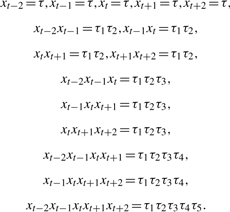As a result, we used a total of 1 686 456 p predicates for this task.

The transition predicate q(y_t−1,y_t) is true if the tags at previous and current positions are y_t−1 and y_t, respectively. Mallet 0.4 provides many options for its users to define how to combine q with p to create features. We used the default setting of Mallet 0.4, which adds an extra ‘O’ tag in the beginning when evaluating q at position t=1, and creates the following two combinations of p and q for the features:

(2)

Since we have three types of tags, there are nine q predicates. We note that HMM-style features described in Lafferty et al. (2001) are different from the above setting:

(3)

where q(·,y_t) is true if the current tag is y_t regardless of what tag y_t−1 is. Usually, we refer to g₂ type of features as observation-independent state-transition features. The difference between these two styles is in g₁ type of features, where state-transition is considered in Mallet's default setting but not in the HMM-style setting. We will show that a CRF model is symmetric with HMM-style features but not with Mallet's default setting. This is crucial because bi-directional parsing using symmetric models produces same results in theory and barely affect the performance.

The total number of all features, in theory, is on the order of 10 millions, as large as the number of p predicates multiplied by nine tag pairings for q predicates.¹ The default setting of Mallet is to generate weights only for those features that are true at least in one sentence in the training corpus. That is, the pattern defined in a feature must occur at least once in the training corpus for the weight of that feature to be generated and used in the model. Since the features are sparse in the sense that only a very small portion of them is true for each sentence, the total number of weights that we used is about 2 million.

2.2 Bi-directional parsing

In an attempt to create two high performance but mutually complementary models to boost the tagging accuracy, we trained two different CRF models using Mallet with the features described above. One model applied forward and the other applied backward parsing. In forward parsing, CRF reads and tags the input tokens in their original order, while in backward parsing, CRF reads and tags the input tokens from right to left, as illustrated in Figure 1. In backward parsing, we changed only the parsing direction but not the tags. In other words, our backward parsing is equivalent to applying ‘I,O,E’ labeling (Kudo and Matsumoto, 2001) to reversed sentences in named entity recognition. As described above, since Mallet is not symmetric, models with different parsing directions are different. We will explain why this is the case in discussion section. Table 2 shows the inside test results of forward and backward parsing models. Surprisingly, the backward parsing model outperforms the forward parsing model not only in F-score but also in both precision and recall.

Table 2.

Inside test results

Method	Precision	Recall	F-score
Forward	86.60	80.77	83.59
Backward	87.33	81.18	84.14
Union	83.49	85.78	84.62
Intersection	90.76	71.86	80.21
Top 10+HUGO	87.73	82.63	85.10

These models were trained by 10 000 example sentences selected at random and tested by the remaining 5000 examples.

2.3 Model integration

We tried different ways to combine the results of bi-directional parsing to maximize the performance. Simple set operations, intersection and union, failed to improve the performance because they lead to trade-off between recall and precision. Here, intersection contains the set of entities tagged by both models and union consisting of the set of entities tagged by either one of the models. Usually, intersection will improve precision but degrade recall while union will improve recall but degrade precision. Table 2 shows the results of intersection and union in our inside test. We also tried to apply co-training (Blum and Mitchell, 1998) but since the output scores of Mallet were not suitable for selecting test results as training examples, co-training seriously degraded the F-score to as low as 60.

Instead, we applied a model integration method based on the output scores and dictionary filtering, in which we used a dictionary-based filter to select entities from the union of the top 10 tagging results obtained by Mallet's n-best option. In fact, the union of the top 10 tagging results of bi-directional parsing achieved a nearly perfect recall at 98.10 for the final test, but with a miserable 13.87 precision, revealing that nearly all true gene entities are in this union. We distilled true gene entities from this union as follows.

1. Parse the input sentence in both directions to obtain the top 10 solutions for each direction with their output scores;

2. compute the intersection of bi-directional parsing and select the solution in the intersection that minimizes the sum of its output scores;

3. for the other 18 solutions, select the labeled terms appearing in a dictionary with its length greater than three.

Step (2) is derived from the optimal model integration (Huang and Hsu, 2002). Let m_i be a model. The optimal integration of m_i's is to select Y such that

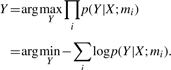The output score of Mallet is the cost for predicting Y: −logp(Y|X)+logZ(X), that is, the negative logarithm of unnormalized probability of tag sequence Y given input sequence X. Therefore, given the same X, logZ(X) will be a constant and comparing the output scores of top Y's is equivalent to comparing their −logp(Y|X). Next, we used approved gene symbols and aliases obtained from HUGO (Eyre et al., 2006) for the last step.

Figure 2 illustrates this model integration step with an example. Suppose that the input sentence is

Fig. 2.

An example illustrates the method of the final model integration step. fw_score and bw_score indicate the output scores of Mallet obtained by forward and backward parsing, respectively, and the highlighted row indicates the tag sequence pair selected by the integrated model.

The gap protein knirps mediates bothquenching and direct repression in theDrosophila embryo.

Its tokenization results are given in the first column. Our bi-directional parsing models generate 10 tagging results for each parsing directions shown as the following columns. In the bottom of the figure are intersection of these results. In this example, there are seven pairs in the intersection, such as column 0 forward, column 1 backward that contain ‘BI,’ and the pair column 1 forward and column 0 backward that contain ‘BII’. It turns out that the pair column 1 forward and column 0 backward has the minimum sum of scores, as the highlighted row in Figure 2. Therefore, our tagger will output ‘BII’ as its answer. Next, our tagger will check the dictionary and found that ‘gap’ in column 5 forward and column 6 backward is a gene name, but its length is not greater than three, so it will not be returned. We note that the gold standard solution of this example is to label ‘gap’ and ‘knirps,’ but in the alternative annotation solutions, labeling ‘gap protein,’ ‘gap protein knirps,’ or ‘protein knirps’ all count as TP in BioCreative 2. Our inside test showed that this method achieved more than 85% in F-score, two percentage points better than the best result in BioCreative 1 (Finkel et al., 2005). Its precision, recall and F-score are shown in Table 2.

3 RESULTS AND DISCUSSION

3.1 BioCreative 2 results

We used the entire training corpus as the training examples and applied the top three performing methods in our inside test to produce three runs of tagging results as our submission to BioCreative 2. The final performance of these methods for the test corpus are shown in Table 3. All of our methods performed better than in the inside test with more training examples becoming available and the best method in the inside test still outperformed the others. Compared to the performance of the rank one entry in BioCreative 2 (Ando, 2007), our best tagger achieves a higher precision and matches more gold standard solutions than alternative annotations. Wilbur et al. (2007) provide detailed comparison of the results of all participants.

Table 3.

Final BioCreative 2 result

Method	Precision	Recall	F-score	Alta (%)
Backward	89.30	83.83	86.48	−
Union	86.10	87.08	86.58	−
Top 10+HUGO	89.30	84.49	86.83	14.02
Rank 1	88.48	85.97	87.21	32.48

^aThe percentage of TP that matched alternative annotations.

3.2 Asymmetric CRF models

One of the most prominent factors that contributes to the good performance of our tagger is the integration of an additional backward parsing model. However, from the graphical model and Equation (1), it appears that a CRF model is symmetric and backward and forward parsing models will produce the same results. In this sub-section, we explain when backward and forward parsing CRF models will be different.

A CRF model with HMM-style features as given in Equation (3) is indeed symmetric in the sense that given a pair of input token sequence X and output tag sequence Y and its reversed pair X^B and Y^B, we have p(Y|X)=p(Y^B|X^B). To establish that this is the case, we need to assume further that:

1. two special tags are attached to the head and tail of Y, as described in Lafferty et al. (2001);

2. the training set of the backward parsing model is the same as the set for the forward parsing model, except that all tokens and tags are in reversed order;

3. all p predicates are either defined on a single token or symmetrically with regard to current position t. Features described in Section 2.1 satisfy this condition.

Then we can always find an isomorphism of features between forward and backward parsing models as follows:

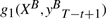• maps to g₁(X,y_t) and

• maps to g₂(y_t−1=T₁ ,y_t=T₂).

We note that position t in forward parsing locates right at position T−t+1 in backward parsing. Features mapped together in the isomorphism always have the same values. If their weights are equal, we can find an isomorphism for M_t in Equation (1), too, and have p(Y|X)=p(Y^B|X^B). Since we train a CRF model to maximize likelihood of training data, in theory, maximum likelihood weights of the two models will be isomorphic, too, and the weights of features mapped to each other will be equal.

In contrast, CRF with Mallet-style features, with general forms given in Equation (2), is no longer symmetric mainly because the input token sequence X is considered in its g₁ type features. Unlike HMM-style features, no isomorphism exists between g₁(X,y_t−1,y_t) and 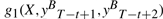because though the pairs y_t−1y_t and are mirror images to each other, current position for g₁(X,y_t−1,y_t) in a forward parsing model is t, which corresponds to position T−t+1 for the backward parsing model, but current position for in a backward parsing model is T−t+2, which is t−1 in forward order, a shift from the corresponding current position t of the forward parsing model. In other words, at the same position t, g₁ features of the forward parsing model considers y_t and y_t−1 but those of the backward parsing model considers y_t and y_t+1. The forward parsing model takes the previous tag into account, while the backward model takes the next tag into account. Therefore, their values are not always equal.

Considering the example given in Figure 1. If we use HMM-style features, then we will have g₂(y₁=O,y₂=B)= true for the tag sequence shown in the figure. Its isomorphic feature for backward parsing with a mirror image tag pair is g₂(y_T−1=B,y_T=O), which is also true for the same tag sequence. But if we use Mallet-style g₁ features and Word as the p predicate, then for the same position with the above pair of tags, we will have that g₁(x₂=gap,y₁=O,y₂=B) is true for forward but g₁(x_T−1=gap,y_T−2=B,y_T−1=O) is false because y_T−2=I not B and y_T−1=B not O when x_t is at gap in backward parsing, as shown in Figure 1. It is impossible to align the features to create an isomorphism between them.

Moreover, Mallet attaches a special tag only to the beginning of a sentence and has special parameters for the cost for selecting a state as the initial state and the cost for selecting a state as the final state. It is more expressive than the model given in Equation (1) and thus not symmetric.

We empirically tested our propositions with CRF++ (Kudo, 2005), another free package for CRF training. We selected CRF++ because it implements Equation (1) exactly and its default feature setting is HMM style. CRF++ also allows its users to select Mallet-style feature setting. Table 4 shows the experimental results, which show that the forward and backward parsing models by CRF++ with HMM-style features produced nearly identical results. In contrast, Mallet and CRF++ with Mallet-style asymmetric features produced different results, with much more different TP and FP than those of CRF++ with HMM-style features. The tiny differences in TP and FP for CRF++ with HMM-style features may simply due to numerical errors in both training and tagging. We also compared the output scores obtained by Mallet and CRF++ for models with different parsing directions and found that at each iteration, the output scores (unnormalized negative log-likelihood) are almost the same for CRF++ with HMM-style features but different for Mallet. The output scores shown in Figure 2 also reveal clear differences between forward and backward parsing models with Mallet.

Table 4.

Comparing forward and backward parsing models

	Forward			Backward			Differencea
	Precision	Recall	F-score	Precision	Recall	F-score	TP	FP	F-score
Mallet	88.88	83.57	86.14	89.34	84.05	86.61	1028	477	+0.47
CRF++:HMM-style	90.15	84.28	87.12	90.22	84.13	87.07	100	46	−0.05
CRF++:Mallet-style	89.48	82.45	85.81	89.89	83.54	86.60	646	401	+0.79

^aColumns under ‘Difference’ show the number of different TP, FP in the tagging results and the difference in F-scores of the forward and backward parsing models. These models were trained by 15 000 example sentences and tested by 5000 examples with the features described in Section 2.1. The split of training/test sets is provided by BioCreative 2. The total number of gold standard true gene entities in the test set is 6331.

3.3 Superiority of backward parsing models

In all of our experiments, we found that if Mallet-style features are used, backward parsing models constantly outperformed their forward parsing counterparts in both recall and precision, though the margin may not be always very large. We had the same finding for models trained by SVM, for which we included a previous tag as one of the features to classify a given token to one of the three tags. That creates a similar asymmetric effect as Mallet-style features for CRF. We even constructed an ensemble of three backward parsing models, consisting of two SVM models and one CRF model, to submit another entry to BioCreative 2 (Huang et al., 2007). Interestingly, it turned out that this ensemble ranked third in BioCreative 2. Even the rank one tagger is not statistically significantly better than this ensemble.

Intuitively, there might be some ‘signal’ at the end of a gene mention that gives advantage to backward parsing. We have shown that with Mallet-style features, forward parsing models take the previous tag into account, while backward models take the next tag into account. This applies to our SVM models as well. Therefore, we used the Kullback-Leibler divergence to measure the information gain from a prior distribution of y_t to its posterior distribution after either previous or next tag becomes available. Let D^B be the information gain when y_t+1 is given, as in the case of backward parsing, and D^F be defined analogously for forward parsing.

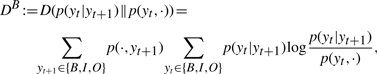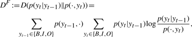where p(y,·) is the probability that the first tag of a randomly selected tag bigram is y, p(·,y) is defined analogously, p(y_t|y_t+1) is the conditional probability that the first tag of a randomly selected tag bigram is y_t given that the second tag is y_t+1, and p(y_t|y_t−1) is defined analogously. We keep the index of position, t in the original (forward) order for both directions. We used 15 000 example sentences in the training corpus from BioCreative 2 to estimate the information gains and obtained that D^B=0.1667>D^F=0.1650, suggesting that a next tag y_t+1 is slightly more informative than a previous tag y_t−1 for predicting y_t, giving backward parsing advantage over forward parsing. We performed a bootstrapping by resampling 5000 example sentences with replacement for 10 000 times from the training corpus. In all trials, we have D^B>D^F. This result is statistically significant because the means for D^B and D^F are 0.1667 and 0.1650, respectively, and the SD for D^B−D^F is 1.1926×10⁻⁴, yielding a t-statistic of 1417.6 that is much larger than t_0.05,9999=2.576. This result is obtained purely from data and is independent of models or feature settings of taggers.

We then compared the prediction accuracy of tag bigrams by forward and backward parsing models to see how information gain plays a role in actual performance. Since the distribution of tags is skewed, we were also interested to investigate if the tagging performance of different parsing directions is specific to any type of tag bigrams. We wanted to know whether it might be the case that it is particularly easy for backward parsing to detect the end of a gene mention by tagging ‘IO’ more accurately than forward parsing. Table 5 shows the confusion matrices of the forward and backward parsing models trained by Mallet with default feature settings and tested on the 5000 sentences in the test corpus of BioCreative 2. Interestingly, though the difference of final F-scores between two models is less than one percentage point, the result shows that backward parsing outperforms forward parsing in F-score for all tag bigrams, revealing that the advantage of backward parsing is not specific to certain tag bigrams.

Table 5.

Confusion matrices of tag bigrams for forward and backward parsing models

	BB	BI	BO	IB	II	IO	OB	OI	OO	r
Forward (yt−1,yt)
BB	3	19	1	0	2	0	0	0	0	12.00
BI	1	2701	58	0	168	2	112	0	458	77.17
BO	0	178	2057	0	75	105	0	0	379	73.62
IB	0	1	0	6	40	3	3	0	2	10.91
II	0	139	24	2	3845	115	136	0	994	73.17
IO	0	3	84	0	160	2682	1	0	514	77.87
OB	0	75	1	3	215	1	5004	0	941	80.19
OI	0	0	0	0	0	0	0	0	0	-
OO	0	278	161	0	651	475	514	0	119999	98.30
p	75.00	79.58	86.21	54.55	74.57	79.28	86.72	-	97.33
F	20.69	78.36	79.42	18.18	73.86	78.57	83.33	0	97.81
Backward (yt,yt+1)
BB	8	14	1	0	1	0	1	0	0	32.00
BI	0	2713	68	0	165	1	91	0	462	77.51
BO	2	150	2110	0	72	85	0	0	376	75.49
IB	0	1	0	8	38	4	3	0	1	14.55
II	0	118	23	6	3886	100	113	0	1009	73.95
IO	0	0	68	1	145	2694	0	0	537	78.20
OB	0	76	0	2	194	0	4841	0	878	80.80
OI	0	0	0	0	0	0	0	0	0	-
OO	0	294	170	0	647	465	514	0	120235	98.29
p	80.00	80.60	86.48	47.06	75.49	80.44	87.02	-	97.36
F	45.71	79.03	80.61	22.22	74.71	79.31	83.80	0	97.82

Rows give true tag bigrams and columns give predicted tag bigrams. All tag bigrams are given in their original (forward) order. The special tags ‘O’ attached to heads and tails of sentences in forward and backward parsing, respectively, were counted. Legend: r=recall, p=precision, F=F-score.

3.4 Model integration

To fully explore the potential of integrating bi-directional parsing models, we applied different feature settings to generate many bi-directional parsing models and integrated them based on their output scores.

Mallet 0.4 provides many feature setting options for users. One of the available options is the ‘Markov orders’ of the features, which concern the dependence relationship between states, that is, tags in our gene mention task, in the graphical model of a CRF model. The default Order is 1, where a state y_t depends only on its adjacent states y_t−1 and y_t+1 given an observed input sequence, and the resulting feature setting is described in Section 2.1. In addition to Order 1, we trained many bi-directional parsing models with Order 0, 2 and 3 using Mallet. Intuitively, orders define the most remote states that a state depends on given an input sequence. The higher the order, the more remote states we have in the dependence relations. We have already shown that Order 1 features have the form f(y_t−1,y_t,X) that takes y_t−1 and y_t as their variables. Features under other order settings have the forms as follows:

• Order 0: f(y_t,X);

• Order 2: f(y_t−2,y_t−1,y_t,X);

• Order 3: f(y_t−3,y_t−2,y_t−1,y_t,X).

In some sense, models with these orders are all reasonable for gene mention tagging. However, orders increase complexity of models and the chance of overfitting. Therefore, for Order 3 models, we reduced the range of contextual features from t−2,…,t+2 to t−1,…,t+1 to simplify the model. But for models with other orders, we basically used the same features described in Section 2.1.

It may appear that Order 0 models are symmetric and thus bi-directional parsing may produce the same result. But for reasons we have explained in Section 3.2, all Mallet models are asymmetric and bi-directional parsing models with Order 0 will still produce different results. Nevertheless, we discarded Order 0 models in our experiment because its performance was too far below the par of the other models.

As a result, we had a total of six models. We then generalized the model integration method described in Section 2.3 to more than two models and applied the method to integrate the six models. In a nutshell, given a tokenized sentence, each model generates top 10 tagging results with their scores. The tagging result appearing in the top 10 lists of all models with the minimum score will be the final tagging result for the given sentence. If no tagging result appears in the top 10 lists of all models, the best tagging result of Order 1 backward model will be selected simply because it is the best performing model in the inside test. We did not use dictionary filtering here.

To further improve the performance, we applied CRF++ to obtain two more divergent yet high performance models. One of the model was obtained by applying the default settings of CRF++. Since the performance of CRF++ models with asymmetric feature settings is mediocre, instead of training bi-directional parsing models using CRF++, we obtained the other model by applying a new CRF training algorithm that we developed, called CTJPGIS (Hsu et al., 2007). CTJPGIS is an accelerated version of generalized iterative scaling (GIS) method (Darroch and Ratcliff, 1972), which is known to be prohibitively slow for training large scale CRF models. CTJPGIS accelerates GIS by approximating the Jacobian matrix of GIS mapping and therefore, its convergence rate performance is comparable with L-BFGS (Nocedal and Wright, 1999), the default training algorithm of CRF++ and Mallet. Since L-BFGS is a second order method that approximate the Hessian matrix of the objective function of CRF, CTJPGIS and L-BFGS searches for the maximum likelihood weights along different paths and the resulting weight vectors may be quite different. We note that although the objective function of CRF is convex, we usually terminated the search before convergence to obtain a better F-score (Sha and Pereira, 2003; Section 4.3). Therefore, it is unlikely that the two algorithms will output the same weight vector. We implemented CTJPGIS by modifying the modules for optimization in CRF++. See Hsu et al. (2007) for details.

Therefore, we had a total of eight models now. We obtained the intersection of two CRF++ models, then produced the final tagging results by computing the union of the intersection and the model integration results of the six Mallet models. The F-score achieved by this new method for the BioCreative 2 test corpus is 88.30, much higher than ours and the rank one entry in BioCreative 2. Our bootstrap test based on random re-sampling of 5000 test sentences with replacement for 10 000 times showed that this result is statistically significant with a p-value equal to 0.0123 compared to the rank one entry and 0.0000 compared to our entry.

Table 6 showed the tagging performance of all models and their integrations. The results show that Order 1 is optimal among models with different order settings. High order models are too complex and perform worse than Order 1 models. Interestingly, all backward parsing models outperformed their forward parsing counterparts regardless of order settings, confirming our analysis results about the superiority of backward parsing. Our model integration method is proved to be effective as the integrated results outperformed any single models. We tried to modify the model voting methods to allow a candidate tagging result to be selected even if it is only in some of the top 10 lists but not all. However, since we only used the top 10 tagging results, the scores for those tagging results not in the top 10 lists were missing and it was difficult to select a correct tagging result based on incomplete sums of scores.

Table 6.

Results of bi-directional parsing models

Method	Precision	Recall	F-score
Order 0
Forward	79.98	73.18	76.43
Backward	81.01	75.00	77.89
Order 1
Forward	88.79	82.99	85.79
Backward	88.76	83.72	86.16
Order 2
Forward	87.00	82.58	84.73
Backward	88.67	83.65	86.09
Order 3
Forward	85.18	80.08	82.55
Backward	87.33	81.68	84.41
CRF++default	90.15	84.28	87.12
ctjpgis	90.60	82.96	86.61
Intersection	92.56	77.60	84.42
0+1+2+3	90.06	84.68	87.28
1+2+3	90.63	84.82	87.63
1+2+3+lc	88.95	87.65	88.30

‘0+1+2+3’ is the integration of the bi-directional models with Order 0–3. ‘1+2+3’ is the integration of models with Order 1–3. 1+2+3+lc is the union of ‘1+2+3’ and the intersection of two CRF++ models. These models were trained and tested with the corpora from BioCreative 2. The feature sets used here were the same for all models but they were slightly different from the set that we used in BioCreative 2 because we removed some minor bugs and redundancies from the original feature extraction program.

4 CONCLUSIONS AND FUTURE WORK

We have described our gene mention tagger in BioCreative 2 in this article and analyzed why integrating bi-directional parsing CRF models can achieve good performance. We showed that different types of feature construction affect whether a CRF model is symmetric, and that with an asymmetric CRF model, forward and backward parsing yield different results. We then explained why backward parsing models enjoy a slight advantage over their forward parsing counterparts with an information gain analysis, and empirically showed that the advantage is not specific to any type of tag bigrams. The new model developed based on our analysis result can achieve even higher F-scores with the same set of training examples.

Given the experimental results reported here and in the literature, we are confident that given more training examples, tagging gene and gene production mentions can be done reliably and the result can be applied to the task of tagging other biological name entities. However, it is not clear whether accurate name entity tagging can contribute directly to the following steps of biological literature mining, including gene normalization and other tasks in BioCreative 2. New models for these steps that are tightly coupled with name entity tagging with a large consistently annotated training corpus may be required to accomplish accuracies sufficiently high for practical biological knowledge discovery.

REFERENCES

- Ando RK. Proceedings of the Second BioCreative Challenge Evaluation Workshop. Madrid, Spain: Centro Nacional de Investigaciones Oncologicas (CNIO); 2007. Biocreative ii gene mention tagging system at IBM watson; pp. 101–103. [Google Scholar]
- Blum A, Mitchell T. Combining labeled and unlabeled data with co-training. COLT: Proceedings of the Workshop on Computational Learning Theory; ACM, New York, NY, USA. 1998. pp. 92–100. [Google Scholar]
- Darroch JN, Ratcliff D. Generalized iterative scaling for log-linear models. Ann. Math. Stat. 1972;43:1470–1480. [Google Scholar]
- Eyre TA, et al. The HUGO gene nomenclature database, 2006 updates. Nucleic Acids Res. 2006;34:D319–D321. doi: 10.1093/nar/gkj147. [DOI] [PMC free article] [PubMed] [Google Scholar]
- Finkel J, et al. Exploring the boundaries: gene and protein identification in biomedical text. BMC Bioinformatics. 2005;6:S5. doi: 10.1186/1471-2105-6-S1-S5. [DOI] [PMC free article] [PubMed] [Google Scholar]
- Hirschman L, et al. Proceedings of the Second BioCreative Challenge Evaluation Workshop. Madrid, Spain: Centro Nacional de Investigaciones Oncologicas (CNIO); 2007. http://biocreative.sourceforge.netlast accessed date: May 18, 2008. [Google Scholar]
- Hsu C-N, et al. Technical Report TR-IIS-07-013. Academia Sinica, Taiwan: Institute of Information Science; 2007. Global and componentwise extrapolations for accelerating training of Bayesian networks and conditional random fields. [Google Scholar]
- Huang H-J, Hsu C-N. Bayesian classification for data from the same unknonw class. IEEE Transactions on Systems, Man, and Cybernetics Part B. 2002;32:137–145. doi: 10.1109/3477.990870. [DOI] [PubMed] [Google Scholar]
- Huang H-S, et al. Proceedings of the Second BioCreative Challenge Evaluation Workshop. Madrid, Spain: Centro Nacional de Investigaciones Oncologicas (CNIO); 2007. High-recall gene mention recognition by unification of multiple backward parsing models; pp. 109–111. [Google Scholar]
- Klinger R, et al. Named entity recognition with combinations of conditional random fields. Proceedings of the Second BioCreative Challenge Evaluation Workshop; Centro Nacional de Investigaciones Oncologicas (CNIO), Madrid, Spain. 2007. pp. 105–107. [Google Scholar]
- Kudo T, Matsumoto Y . NAACL'01: Second meeting of the North American Chapter of the Association for Computational Linguistics on Language technologies 2001. Pittsburgh, Pennsylvania. Morristown, NJ, USA: Association for Computational Linguistics; 2001. . Chunking with support vector machines; pp. 1–8. http://dx.doi.org/10.3115/1073336.1073361(last accessed date May 18, 2008) [Google Scholar]
- Kudo T. Crf++: yet another crf toolkit. 2005 http://crfpp.sourceforge.net/
- Kuo C-J, et al. Rich feature set, unification of bidirectional parsing and dictionary filtering for high f-score gene mention tagging. Proceedings of the Second BioCreative Challenge Evaluation Workshop; Centro Nacional de Investigaciones Oncologicas (CNIO), Madrid, Spain. 2007. pp. 105–107. [Google Scholar]
- Lafferty J, et al. Conditional random fields: probabilistic models for segmenting and labeling sequence data. ICML'01: Proceedings of 18th International Conference on Machine Learning; San Francisco, CA, USA. Morgan Kaufmann Publishers Inc; 2001. pp. 282–289. [Google Scholar]
- McCallum AK. Mallet: a machine learning for language toolkit. 2002 http://mallet.cs.umass.edu. (last accessed date May 18, 2008)
- McDonald R, Pereira F. Identifying gene and protein mentions in text using conditional random fields. BMC Bioinformatics. 2005;6:S6. doi: 10.1186/1471-2105-6-S1-S6. [DOI] [PMC free article] [PubMed] [Google Scholar]
- Mitsumori T, et al. Gene/protein name recognition based on support vector machine using dictionary as features. BMC Bioinformatics. 2005;6:S8. doi: 10.1186/1471-2105-6-S1-S8. [DOI] [PMC free article] [PubMed] [Google Scholar]
- Nocedal J, Wright SJ. Numerical Optimization. New York, NY, USA: Springer; 1999. [Google Scholar]
- Sha F, Pereira F. Shallow parsing with conditional random fields. Proceedings of Human Language Technology, the North American Chapter of the Association for Computational Linguistics (NAACL'03) 2003:213–220. Edmonton, Canada. Association for Computational Linguistics, Morristown, NJ, USA http://dx.doi.org/10.3115/1073445.1073473.
- Tsuruoka Y, et al. Advances in Informatics, Lecture Notes in Computer Science. Vol. 3746. Springer: Berlin / Heidelberg; 2005. Developing a robust part-of-speech tagger for biomedical text; pp. 382–392. [Google Scholar]
- Wilbur J, et al. Biocreative 2. gene mention task. Proceedings of the Second BioCreative Challenge Evaluation Workshop; Centro Nacional de Investigaciones Oncologicas (CNIO), Madrid, Spain. 2007. pp. 7–16. [Google Scholar]
- Zhou GD. Recognizing names in biomedical texts using mutual information independence model and svm plus sigmoid. Int. J. Med. Inform. 2006;75:456–467. doi: 10.1016/j.ijmedinf.2005.06.012. [DOI] [PubMed] [Google Scholar]