BLASTing small molecules—statistics and extreme statistics of chemical similarity scores

Abstract

Motivation: Small organic molecules, from nucleotides and amino acids to metabolites and drugs, play a fundamental role in chemistry, biology and medicine. As databases of small molecules continue to grow and become more open, it is important to develop the tools to search them efficiently. In order to develop a BLAST-like tool for small molecules, one must first understand the statistical behavior of molecular similarity scores.

Results: We develop a new detailed theory of molecular similarity scores that can be applied to a variety of molecular representations and similarity measures. For concreteness, we focus on the most widely used measure—the Tanimoto measure applied to chem-ical fingerprints. In both the case of empirical fingerprints and fingerprints generated by several stochastic models, we derive accurate approximations for both the distribution and extreme value distribution of similarity scores. These approximation are derived using a ratio of correlated Gaussians approach. The theory enables the calculation of significance scores, such as Z-scores and P-values, and the estimation of the top hits list size. Empirical results obtained using both the random models and real data from the ChemDB database are given to corroborate the theory and show how it can be applied to mine chemical space.

Availability: Data and related resources are available through http://cdb.ics.uci.edu

Contact: pfbaldi@ics.uci.edu

1 INTRODUCTION

Small organic molecules, from nucleotides and amino acids to metabolites and drugs, play a fundamental role in chemistry, biology, and medicine. As chemical repositories of small molecules continue to grow and become more open (Chen et al., 2005, 2007; Irwin and Shoichet, 2005), it becomes increasingly important to develop the tools to search them efficiently. In one of the most typical settings, a query molecule is used to search millions of other compounds not only for exact matches, but also for approximate matches. In a drug discovery project, for instance, one may be interested in retrieving all the commercially-available compounds that are ‘similar’ to a given lead, with the aim of finding compounds with better physical, chemical, biological or pharmacological properties.

Likewise, in a reverse synthesis project, one may be interested in identifying small molecules that can explain a mass spectrometry signature, or can be used used as building blocks for the artificial synthesis of a metabolite or a natural product. The idea of searching for molecular ‘cousins’ is of course not new, and constitutes one of the pillars of bioinformatics where one routinely searches for homologs of nucleotide or amino acid sequences. Search tools such as BLAST (Altschul et al., 1997) and its significance ‘e-scores’ have become de facto standards of modern biology, and have driven the exponential expansion of bioinformatics.

While molecular similarity is different from molecular homology in that it is not predicated on an underlying evolutionary process, there is no reason to believe that a BLAST-like tool for small molecules cannot be developed. Indeed, many different representations and similarity measures have been developed in chemoinformatics over the years (Leach and Gillet, 2005). Yet no consensus tool such as BLAST has emerged. One of the reasons behind the lack of consensus is that there has been no systematic, large-scale, open study of molecular similarity scores, and their statistical distributions and significance levels. As a result, the majority of existing chemical search engines do not return a score with the molecules they retrieve, let alone any measure of significance. Examples of fundamental questions one would like to address include: What threshold should one use to assess significance in a typical search? Is a Tanimoto score of 0.4 significant or not? How many molecules should be expected to have a score above 0.4 and under which assumptions? How does the answer depend on the size of the database being queried? How does the answer depend on the type of query used? A clear answer to these questions is critical for unifying existing chemical databases and search methods, for assessing the significance of a similarity score, and ultimately for helping to better understand the nature of chemical space.

Here we address these questions by conducting a systematic statistical study of chemical similarity scores and their extreme values as a function of, for instance, database size. To do so, in Section 2, we first define the molecular representations and similarity scores to be used in the study. Then, in Section 3, we introduce the probabilistic models required to both approximate empirical distributions of similarity scores and to create random models of the background similarity scores against which significance can be assessed. In Section 4, we develop the theory for the distribution of the similarity scores, and in Section 5 the theory for the distribution of the extreme values of these similarity scores. Experimental results to illustrate and corroborate the theory are described in Section 6 followed by a discussion and conclusions in Section 7.

2 MOLECULAR REPRESENTATIONS AND SIMILARITY SCORES

Many different representations and similarity scores have been developed in chemoinformatics (Leach and Gillet, 2005). The methods to be described are very broadly applicable but, for brevity, we illustrate the theory using one of the most commonly used frameworks across chemoinformatics platforms, namely binary fingerprint representations with Tanimoto similarity scores.

2.1 Molecular representations: fingerprints

To search large databases of compounds by similarity, most modern chemoinformatics systems use a fingerprint vector representation (Baldi et al., 2007; Fligner et al., 2002; Flower, 1998; James et al., 2004; Leach and Gillet, 2005; Xue et al., 2003, 2004) whereby a molecule is represented by a vector whose components index the presence/absence, or the number of occurrences, of a particular functional group, feature or substructure in the molecular bond graph. Because binary fingerprints are used in the great majority of cases, here we present the theory for these fingerprints, but it should be clear that the theory can readily be adapted to fingerprint based on counts. We use 𝒜 to denote a molecule and to denote the corresponding fingerprint vector. We let A denote the number of bits set to 1 (1-bits) in the fingerprint ().

In early chemoinformatics systems, fingerprint vectors were relatively short, containing typically a few dozen components selected from a small set of features, hand-picked by chemists. In most modern systems, however, the major trend is towards the combinatorial construction of extremely long feature vectors with a number of components N that can vary in the 10³–10⁶ range, depending on the set of features. Examples of typical features include all possible labeled paths or labeled trees, up to a certain depth. The advantage of these much longer, combinatorially-based representations is 2-fold. First, they do not require expert chemical knowledge, which may be incomplete or unavailable. Second, they can support extremely large numbers of compounds, such as those that are starting to become available in public repositories and commercial catalogs, as well as the recursively enumerable space of virtual molecules (Bohacek et al., 1996). The particular nature of the fingerprint components is not essential for the theory. To illustrate the principles, in the simulations we use both fingerprints based on labeled paths and fingerprints based on labeled shallow trees with qualitatively similar results. For brevity and consistency, the examples reported in the Results are derived primarily using fingerprints based on paths.

2.2 Fingerprint compression

In many chemoinformatics systems, the long sparse fingerprint vectors are often compressed to much shorter and denser binary fingerprint vectors. The most widely used method of compression is a lossy compression method based on the application of the logical OR operator to the binary fingerprint vector after modulo wrapping to 1024 bits (James et al., 2004). Thus component i of the compressed fingerprint is set to 0 if and only if all the positions i modulo 1024 are set to 0 in the uncompressed fingerprint. Other more efficient lossless methods of compression have recently been developed (Baldi et al., 2007). With the proper and obvious adjustments, our results are applicable to both lossy compressed and uncompressed fingerprints. Because lossy compressed representations are the most widely used, we report the majority of our results using modulo-OR compressed binary fingerprints of length N=1024. Due to their smaller size, these also have the advantage of speeding up Monte Carlo sampling simulations.

2.3 Similarity scores

Several similarity measures have been developed for molecular fingerprints (Holliday et al., 2002; Leach and Gillet, 2005; Swamidass and Baldi, 2007). Given two molecules 𝒜 and ℬ, the Tanimoto similarity measure is given by

(1)

Here (A∩B) denotes the size of the intersection, i.e. the number of 1-bits common to and , and A∪B denotes the size of the union, i.e. the number of 1-bits in or . Because the Tanimoto similarity is by far the most widely used, the theory and experimental results reported here are based on Tanimoto similarity. However, the same theory can readily be applied to all the other measures. To see this, it suffices to note that the other measures consist of algebraic expressions built from A∪B and A∩B, as well as other obvious terms such as A, B, and sometimes N. For instance, the Tversky measure (Rouvray, 1992; Tversky, 1977) is defined as , where the parameters α and β can be used to tune the search towards the sub-structures or super-structures in the query molecule. The theory to be presented begins precisely by studying the statistical distribution and properties of the intersection and the union, in particular their mean, variance and covariance. Thus, the distribution and statistical properties of all the other similarity measures can readily be derived from the distributions analyzed in this article. For this reason, we focus on the Tanimoto score, which can be viewed as the chemoinformatics analog of the alignment score in bioinformatics.

2.4 Data

In the simulations and results, we illustrate the methods using fingerprints of molecules randomly sampled from the ∼5 M molecules available in the ChemDB database (Chen et al., 2005, 2007), or randomly generated using the stochastic generative models described in Section 3. The empirical fingerprints are generated by indexing all the labeled paths of length up to eight, or all the labeled trees of depths up to two present in the molecular bond graph. The labels on the vertices correspond to the atom type (e.g. C, N, O) while the labels on the edges correspond to the bond type (e.g. single, double, triple). The exact details of the fingerprints, which are not important for this study, can be found in (Baldi et al., 2007) and references therein. Except where noted, both the empirical and model fingerprints are generated using 1024-bit modulo compression. In the simulations, the reported distributions are typically determined using random samples of n=100 query fingerprints against background databases that range in size from 5000 to 1 million fingerprints.

3 STATISTICAL MODELS OF FINGERPRINTS

Statistical models of fingerprints are essential for a variety of tasks. For instance, in fingerprint compression, fingerprints can be viewed as ‘messages’ produced by a stochastic source and understanding the statistical regularities of the source is essential for deriving efficient compression algorithms that use short codewords for the most frequent events. Here, statistical models are essential in at least two different ways: (1) to model and approximate the distribution of similarity scores; and (2) to assess significance against ‘chance’, where chance can be defined in various ways. Similar observations, of course, can be made in sequence analysis to, for instance, assess what is the probability of observing a particular alignment score against a random generative background model of nucleotide or amino acid sequences. It is worth noting that as a default, we assume that the distribution over the queries is the same as the distribution over the molecules in the database. However, these statistical models can also be used to model particular distributions over the space of queries that may differ from the overall distribution.

3.1 One-parameter Bernoulli trials and binomial model

The simplest statistical model for binary fingerprints is a sequence of independent identically distributed Bernoulli trials (coin flips) with probability p of producing a 1-bit, and q=1−p of producing a 0-bit. This model can be applied to both long fingerprints with a very low p, or to the modulo-OR compressed fingerprints of length 1024 with a higher value of p. The coin flip model is consistent with fingerprint features that are randomly ordered and statistically exchangeable, in fact even independent, and leads to a binomial model ℬ(N, p), with only two parameters N and p, for the total number of 1-bits in the corresponding fingerprints. The Bernoulli/binomial model can be used, either to approximate the distribution of fingerprints in an entire database such as ChemDB, or the distribution of fingerprints given a value for A by using p=A/N. In the former case, as we will show (Fig. 1), the binomial model does not reproduce the variance of A across the database very well since in a binomial model, the variance Npq is always at most equal to the expectation Np, whereas in large databases of compounds we tend to observe a larger variance. A better model is a normal distribution 𝒩(μ,σ²) where the mean μ=Np and variance σ²≠Npq are fitted to the empirical distribution across the database. In the latter case, by generating fingerprints with probability p=A/N, the number of 1-bits is not constant and varies around the mean value A, introducing some additional variability with respect to the case where A is held fixed (Section 3.3).

Fig. 1.

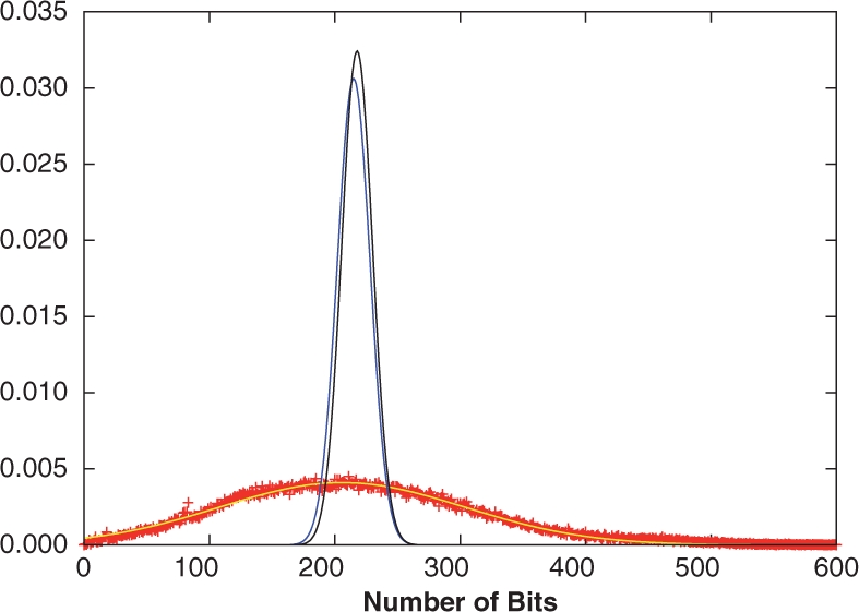
Distributions of 1-bits from the ChemDB fingerprints (red ‘+’), and the Binomial (blue) and multiple Bernoulli (black) fingerprint models. The empirical distribution was also fit to a Gaussian (yellow), which approximates the data well. While the model distribution means are close to the empirical mean, the distribution widths are significantly smaller.

3.2 Multiple-parameter Bernoulli model

While the coin flip model is useful to derive a number of approximations, it is clear that chemical fingerprints have a more complex structure and their components are not exactly exchangeable since the individual feature probabilities p₁,…,p_N are not identical and equal to p but vary and, when reordered in decreasing order, follow roughly a power-law distribution (Baldi et al., 2007), especially in the uncompressed case. The probability of the j-ranked component is given approximately by p_j=Cj^−α resulting in a line with slope −α in a log-log plot. Thus, the statistical model at the next level of approximation is that of a sequence of non-stationary coin flips where the probability p_j of each coin flip varies. The multiple-parameter Bernoulli model has N parameters: p₁, p₂, …, and p_N. In this case, the expectation of the total number A of 1-bits is given by ∑_ip_i and its variance by . This model is useful in simulations and compression (Baldi et al., 2007), but cannot be treated analytically due to its large number of parameters, unless the approximation p_j=Cj^−α is used. A distribution over queries different from the overall distribution could be modeled using a multiple-parameter Bernoulli model with different parameters r₁, …, r_N.

3.3 Conditional distribution model

Both the binomial and multiple-parameter Bernoulli models consider the fingerprint components as independent random variables. The conditional distribution model is an exchangeable model where the components are weakly coupled. To generate a fingerprint vector under this model, we first sample A, the total number of 1-bits, using a given distribution, typically a Gaussian. Then we sample uniformly over fingerprint vectors containing A 1-bits (which can be realized by randomly permuting the components of real fingerprints). The conditional Gaussian model has only three parameters: the mean μ, the variance σ² and N. Compared to the binomial model, the additional parameter in the conditional Gaussian model allows for a better fit of the variance of A in the data.

3.4 Spin model

More complex, second order, models are possible but will not be considered here. These models are essentially spin models from statistical physics, and are also known as Markov random fields or Boltzmann machines (Ackley et al., 1985; Frey, 1998). In these models, one would have to also take into account the correlations between pairs of features which can be superimposed over the multiple Bernoulli model. In real data, these correlations are not exchangeable, and thus behave differently from those introduced in the conditional distribution model. In real data, however, and especially in the case of uncompressed fingerprints, these correlations are close to 0 both on average and in the typical case, and will not be considered here any further. In general, these models cannot be treated exactly.

4 THEORY: SIMILARITY SCORE DISTRIBUTION

As we have seen, most similarity measures between two fingerprints are built by first computing the intersection and the union. Thus, the basic strategy, is to first study the distribution of the intersection and the union under some of the statistical models given above. Note that the intersection and union, in general, are not two independent random variables, but have a non-zero correlation that must be estimated. Knowledge of the distributions of the intersection and unions can then be used to study the Tanimoto measure and derive its approximate distribution under various assumptions.

4.1 Single-parameter Bernoulli/binomial model

Under the exchangeable independent model, molecules B in the database can be modeled by a binomial ℬ(N,p) which can be approximated by a normal distribution 𝒩(Np, Npq) for large N. Consider a query A with distribution ℬ(N,r) which can be approximated by 𝒩(Nr, Nrs) (s=1−r) for large N. Then the intersection I=A∩B=∑_iI_i=∑_i(A_i∩B_i) is a random variable with binomial distribution ℬ(N, pr), which can be approximated by a normal distribution 𝒩(Npr, Npr(1−pr)) for large N, as well as a Poisson distribution 𝒫(Npr) when N is large and pr is very small. Then the union U=A∪B=∑_iU_i=∑_i (A_i∪B_i) is a random variable with binomial distribution ℬ(N,1−qs)=ℬ(N,p+r−pr), which can be approximated by a normal distribution 𝒩(N(1−qs), N(1−qs)qs) for large N, and a Poisson distribution 𝒫(N(p+r−pr)) when N is large and p+r−pr is small.

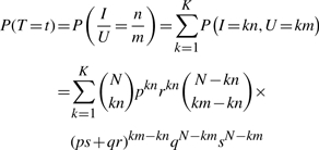
Under the binomial model, we can get an exact expression for the distribution of the Tanimoto scores. Note that the Tanimoto score T=I/U can only take rational values t between 0 and 1. Assuming that n and m are irreducible, with 0≤n≤m and t=n/m, the probability P(T=t) is given exactly by

(2)

where K is the largest integer such that Km≤N, i.e. . Clearly if t is not rational, this probability is 0. Thus, in principle, from this distribution we can derive all the properties of the score distribution, including its mean and variance, under the assumptions of the binomial model.

In practice, it is easier to approximate the numerator I and denominator U by Gaussian distributions and view the Tanimoto score as the ratio of two correlated Gaussians. Thus, we next need to compute the covariance between I and U under the binomial model. Noticing that I_i and U_j are independent for i≠j, we have

(3)

A direct calculation gives Cov(I_i,U_i)=E(I_iU_i)−E(I_i)E(U_i)=pr(1−p−r+pr) so that

(4)

4.2 Multiple-parameter Bernoulli model

The analysis above for the binomial model can easily be extended to the multiple-parameter Bernoulli model by using similar expressions for the mean, variance and covariance of the individual variables I_i and U_i, and combining them using the linearity of the expectation and the independence of components associated with different indices. In this case, we let p₁,p₂,… ,p_N be the vector of probabilities for the database and r₁,r₂,…,r_N the vector of probabilities for the queries. The mean and variance of I are given by ∑_ip_ir_i and ∑_ip_ir_i(1−p_ir_i), respectively. Thus, I can be approximated by a normal distribution 𝒩(∑_ip_ir_i,∑_ip_ir_i(1−p_ir_i)). Likewise, the mean and variance of U are given by ∑_i (1−q_is_i) and ∑_i (1−q_is_i)q_is_i, respectively. Thus, U can be approximated by a normal distribution 𝒩(∑_i (1−q_is_i),∑_i (1−q_is_i)q_is_i). Finally, for the individual covariance terms we have Cov(I_i,U_i)=p_ir_i(1−p_i−r_i+p_ir_i) and Cov(I_i,U_j)=0 for i≠j. Therefore, the full covariance is given by the sum Cov(I,U)=∑_ip_ir_i(1−p_i−r_i+p_ir_i).

4.3 Conditional Gaussian model and hypergeometric distribution

In some cases, it is useful to condition the Tanimoto scores on a fixed value of A. For example, when A is very small or very large, the Tanimoto distribution may differ from that for an average query, and a better approximation may be obtained by conditioning the distribution on A. The binomial model ℬ(N, r=A/N) is not an ideal model since it introduces additional fluctuations on the value A. To address this issue, under the exchangeable hypothesis (no need for independence), it is easy to see that for fixed A and B the intersection I=A∩B has a hypergeometric distribution with probabilities given by

(5)

for A+B−N≤k≤inf(A, B), and 0 otherwise. The mean and variance of the hypergeometric distribution are given by AB/N and AB(N−A)(N−B)/N²(N−1). The union can be studied from the intersection by writing U=A+B−I, so that P(U=k|A,B)=P(I=A+B−k|A,B). Thus, when A and B are fixed, we have E(U)=A+B−E(I), Var(U)=Var(I), and Cov(I,U)=−Var(I).

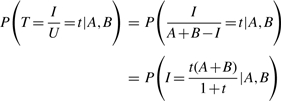
To study the Tanimoto scores directly, we have the conditional density

(6)

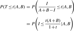
and conditional cumulative distribution

(7)

Therefore, the probability distribution for the similarity T can be derived from the hypergeometric distribution of I, given A, B and N. In particular, we have the conditional distribution

(8)

where the sum is over the distribution P(B). To model this distribution, we can use the binomial model . But it is often preferable, as previously discussed, to use a more flexible Gaussian model with

(9)

where the mean and standard deviation are fitted to the empirical values. The unconditional distribution of Tanimoto scores is given by a second integration over the distribution P(A) of queries

(10)

Again, for convenience, we will assume that P(A)=P(B) as a default, i.e. we will use the same distribution for the queries and the molecules in the database, but in specific applications this does not have to be so. Below, we refer to this unconditional model with P(A)=P(B) represented as Gaussians as the hypergeometric/Gaussian model.

4.4 Ratio-of-Gaussians approximation

Whether one uses the binomial, multiple Bernoulli or hyper-geometric models, or the empirical data, in the end, the Tanimoto score distribution can be approximated by the distribution of the ratio-of-correlated Gaussians approximating the numerator and the denominator, respectively. The different models will yield different estimates of the mean, variance and covariance of the Gaussians. Note that the same approach can be used to approximate directly the empirical distribution of the Tanimoto scores in a database such as ChemDB. The only difference is that instead of fitting the correlated Gaussian parameters to the intersection and union distributions under a probabilistic model, we fit the parameters to the empirical intersection and union distributions in ChemDB.

The density of the ratio of correlated Gaussian distributions can be obtained analytically, although its expression is somewhat involved (Cedilnik et al., 2004; Hinkley, 1969; Marsaglia, 1965; Pham-Gia et al., 2006). The probability density for T=X/Y, where , , and ρ=Corr(X,Y)≠±1 is given by the product of two terms

(11)

or

(12)

where

(13)

(14)

and

(15)

Thus, anytime we can approximate the distribution of the intersection and the union by two correlated Normal distributions, the distribution of the Tanimoto scores can be approximated using Equations (11)–(15) with X=I and Y=U. This approach can be used, for instance, to derive the mean and standard deviation of the Tanimoto scores under various assumptions including: (1) the binomial and multiple-parameter Bernoulli models with p=r (or p_i=r_i) for the average Tanimoto scores across all queries; (2) the binomial and multiple-parameter Bernoulli models with p≠r (or p_i≠r_i) for queries modeled by a different Bernoulli model than the one used for the database being searched; (3) the hypergeometric model with A fixed, or A integrated over the database distribution, or a distribution over queries; and (4) the empirically-derived Gaussian models for the union and intersection averaged over the entire database, or focused on a particular class of molecules. Finally, from the ratio of Gaussians approximation of the score distribution, it is possible to estimate the number of molecules that have a score greater than or equal to t.

5 THEORY: SIGNIFICANCE, Z-SCORES, EXTREME VALUE DISTRIBUTIONS, AND P-VALUES

There are at least two basic approaches for detecting when a similarity score is significant: Z-scores, and P-values associated with the extreme value distributions.

5.1 Z-scores

In the Z-score approach, one simply looks at the distance of a score from the mean of the scores, in numbers of standard deviations. Therefore, the Z-score is given by

(16)

The parameters μ and σ can be determined either empirically from a database of fingerprints, or using the statistical models described above. While Z-scores can be useful, their focus is on the mean and standard deviation of the distribution of the scores, not on the tail of extreme values.

5.2 Extreme value distributions and P-values

The second approach is to compute P-values. For a given score t, its P-value is the probability of finding a score equal or greater to t under a random model. Thus in this case, one is interested in modeling the tail of the distribution of the scores, and more precisely the distribution of the maximum score (Coles, 2001; Galambos 1978; Leadbetter et al., 1983). This distribution depends on the size of the database being searched since for a given query, and everything else being equal, we can expect the maximum similarity value to increase with the database size.

Consider a query molecule 𝒜 and a database containing D molecules, yielding D similarity scores t₁,…,t_D. The cumulative distribution of the maximum F_max(t)=P(max≤t) is given by

(17)

under the usual assumption that the scores are independent and identically distributed. Here F_T(t) is the cumulative distribution of a single score. A P-value is obtained by computing the probability p=1−F_max(t) that the maximum score is larger than t under a chance model.

The density of the maximum is obtained by differentiation

(18)

where f_T(t) is the density of a single score. In the case of Tanimoto similarity scores, f_T(t) can be approximated by the ratio-of-Gaussians approach described above, and F_T(t) is obtained from f_T(t) by integration. F_T(t) can also be approximated by (Hinkley, 1969)

(19)

where is the cumulative distribution of the normalized Gaussian distribution. This approximation is good when the denominator of the ratio-of-Gaussians is positive, with its standard deviation much larger than its average. By combining Equations (11), (18) and (19), we get:

(20)

Finally, because the Tanimoto scores are bounded by one, the theory of extreme value distributions shows that the cumulative distribution of the normalized maximum score n_D, normalized linearly in the form n_D=a_Dmax+b_D using appropriate sequences a_D and b_D of normalizing constants, converges to a type-III extreme value distribution, or Weibull distribution function, of the form

(21)

6 EXPERIMENTAL RESULTS

6.1 Distributions of A, A∩B and A∪B

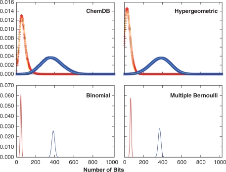
In this section we investigate the distributions of the number of fingerprint bits set to 1 per molecule (1-bits), as well as the intersection and union distributions, using empirical fingerprints extracted from ChemDB and the fingerprint models described in Section 3. Figure 1 compares the empirical 1-bit distribution to the distributions arising from the binomial and multiple parameter Bernoulli models. The two model distributions are similar, and match the empirical distribution mean, but not the variance, which is larger for the empirical fingerprints due to the diversity of molecule sizes in the database. Similar results are also observed for the intersection and union distributions (Fig. 2), where the binomial and multiple Bernoulli models provide a good approximation of the distribution means, but have much smaller standard deviations. To better model the width of the empirical distributions, the hypergeometric model is used in conjunction with a Gaussian distribution to describe the underlying fingerprints. As discussed in Section 4.3 and apparent from Figure 1, a more flexible Gaussian model accurately describes the empirical fingerprint distribution. Under the hypergeometric model, the intersection and union distributions are determined by integrating Equation (5), and its union analog, over P(A) and P(B) modeled by the same Gaussian distribution fit to the empirical 1-bit distribution. Compared to the binomial and multiple Bernoulli distributions, the hypergeometric/Gaussian distributions are much wider, and are very similar to those observed empirically (Fig. 2). In all cases, the distributions are well approximated by Gaussians, with χ² values in the 10⁻⁴–10⁻⁶ range (see Table 1 for parameters), though deviations are seen in the tails of the distributions for the empirical results.

Fig. 2.

Intersection (red) and union (blue) distributions calculated empirically from the ChemDB fingerprints, and from the various fingerprint models described above. For the ChemDB results, the distributions were empirically sampled (‘+’), and fit to Gaussians (solid lines). The calculated hypergeometric/Gaussian distributions are shown with ‘+’ symbols, and the Gaussian fits in solid lines, which are good approximations of the empirical distributions. In the case of the binomial and multiple Bernoulli models, the Gaussian approximations are shown (solid lines), which can be calculated directly from the model parameters. In all cases, the distributions are well approximated by Gaussian distributions.

Table 1.

Distribution parameters of Gaussian approximations for the 1-bit, intersection, and union distributions

Distribution	μ	σ
1-Bits (ChemDB)	205.8	97.9
1-Bits (Binomial)	215.0	13.0
1-Bits (Multiple Bernoulli)	217.7	12.3
Intersection (ChemDB)	58.2	31.3
Intersection (Binomial)	45.1	6.6
Intersection (Multiple Bernoulli)	66.4	6.9
Intersection (Hypergeometric/Gaussian)	31.2	31.8
Union (ChemDB)	364.7	109.0
Union (Binomial)	385.7	15.8
Union (Multiple Bernoulli)	369.1	14.3
Union (Hypergeometric/Gaussian)	380.5	107.2

The ChemDB parameters were obtained from Gaussian fits of the sampled distributions. The binomial and multiple Bernoulli parameters were calculated directly from the models, and the hypergeometric/Gaussian parameters were obtained from Gaussian fits to the distribution calculated directly from the equations in Section 4.3.

6.2 Ratio-of-Gaussians

From the Gaussian approximations of the intersection and union distributions, determined either empirically or from the fingerprint models, it is possible to model the Tanimoto score distribution as a ratio-of-correlated Gaussians. To test how well this model works in practice, the Tanimoto distributions are first sampled using empirical ChemDB fingerprints, and randomly generated fingerprints under the binomial and multiple Bernoulli models. The Tanimoto distribution for the hypergeometric/Gaussian model is calculated directly from Equation (10). Next, the corresponding ratio-of-Gaussians approximations, f_T(t), are calculated according to Equation (12) using the intersection and union parameters given in Table 1, along with the intersection and union correlations, calculated empirically for the ChemDB and hypergeometric/Gaussian results, and analytically for the binomial and multiple Bernoulli models (Table 2). In each case, the ratio-of-Gaussians model provides a good approximation of the observed Tanimoto distributions (Fig. 3). Therefore, as these results show, it is possible to accurately predict the distribution of Tanimoto scores from the intersection and union distributions, and their correlation with one another, either determined empirically, or under a stochastic generative model of fingerprints.

Table 2.

Empirical and model Tanimoto score distribution parameters

Distribution	μ	σ	ρ
Tanimoto (ChemDB)	0.17	0.052	0.82
Tanimoto (fT(t)ChemDB)	0.16	0.055	0.82
Tanimoto (Binomial)	0.12	0.017	0.28
Tanimoto (Multiple Bernoulli)	0.18	0.018	0.25
Tanimoto (Hypergeometric/Gaussian)	0.10	0.050	0.90

The parameters were determined from Gaussian fits to the distributions, except for the ratio-of-Gaussians parameters (f_T(t)_ChemDB), which were determined directly from the analytical formula for f_T(t). The intersection and union correlations are also given. The ratio-of-Gaussians approximation gives accurate estimates of the empirical distribution parameters. With the empirical bit probabilities, the multiple Bernoulli model gives a good approximation of the empirical mean, but the distribution width is too small. Conversely, the use of a Gaussian to model the query and database fingerprints allows to the hypergeometric/Gaussian model to reproduce the empirical distribution width, though the distribution mean is smaller than the empirical value.

Fig. 3.

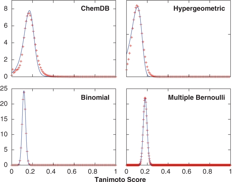
Distribution of Tanimoto scores (red ‘+’) and their ratio-of-Gaussians approximations (blue lines). The Tanimoto distributions were sampled using empirical fingerprints for the ChemDB results, and randomly generated fingerprints for the binomial and multiple Bernoulli models. The hypergeometric/Gaussian distribution was calculated directly from Equation (10). The ratio-of-Gaussians model provides excellent approximations of the Tanimoto distributions.

6.3 Extreme value distributions

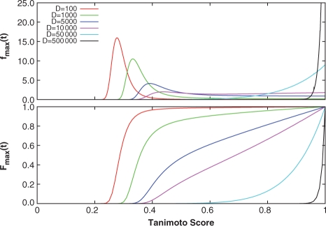
Once the distribution of Tanimoto scores is determined, either empirically from a database of molecules, or based upon a mathematical model, it is possible to assess the significance of a particular similarity score in relation to this distribution. One way to assess a score's significance is through its P-value, which can be calculated from the cumulative distribution of the maximum scores as p=1−F_max(t). From the ratio-of-Gaussians approximation calculated from the fitted ChemDB parameters, the distributions of the maximum scores f_max(t) and their cumulative distributions F_max(t) were calculated for various database sizes D (Fig. 4). For small database sizes (D<5000), the maximum scores lie in the 0.2–0.4 interval. Upon further increase in D, the maximum score distribution widens, and becomes nearly uniform above t=0.4. Finally, for D>50000, f_max(t) gets pushed closer to t=1.0, and begins to concentrate around this upper score limit. The resulting cumulative distributions indicate that database size plays an important role in determining the P-value of a similarity score. For small databases, a large similarity score may result in a very small P-value, while for a large database, the same score may produce a much larger P-value.

Fig. 4.

Maximum and cumulative maximum Tanimoto score distributions derived from Equations (17) and (18) using the empirical ratio-of-Gaussian parameters for different database sizes D (red: D=100, green: D=1000, blue: D=5000, magenta: D=10000, cyan: D=50000, black: D=500000). As D increases for f_max(t), the distribution shifts from being concentrated around relatively low scores, to scores concentrated around 1.0. For small database sizes, the cumulative distributions F_max(t) quickly increase and saturate toward lower scores, while at larger databases sizes, the distributions remain small over most of the score range and rapidly increase as they approach 1.0.

When investigating the distribution of maximum scores, another important question to consider is how many hits, above a given similarity threshold, one should expect on average. In Table 3, the percentage of molecules with similarity scores above a lower limit t_min are given, estimated using the score distribution predicted by the ratio-of-Gaussians model with the fitted ChemDB parameters. As the threshold increases, the number of expected hits rapidly falls off. The values in Table 3 represent a first order approximation of the number of expected hits in the tails of the Tanimoto score distribution for an average query. However, potentially large deviations in these values are possible depending upon the size of the query A. More accurate estimates of the number of hits in the distribution tails may be obtained using the theory outlined in Section 4.3 for the distributions conditioned on A (results not shown).

Table 3.

Percentages of molecules with similarity scores above t_min from the ratio-of-Gaussians approximation with the fitted ChemDB parameters

tmin	Gaussian ratio (%)	No. Hits (D=1 M)
0.4	0.033	330
0.5	0.015	150
0.6	0.010	100
0.7	0.007	70
0.8	0.004	40
0.9	0.002	20

The number of expected molecule hits is also shown for a database of size D=1M. These values provide a qualitative estimate of the number of hits expected for a typical query above the given Tanimoto thresholds.

7 DISCUSSION AND CONCLUSIONS

We have presented a general mathematical framework, along with several stochastic models for chemical fingerprint, from which the distribution of similarity scores, and the extreme value distributions can be accurately predicted. As shown in Figure 2, the intersection and union distributions are well described by Gaussians, both in the empirical case and for the fingerprint models. Using the Gaussian parameters and the correlation between the intersection and union distributions, the ratio-of-Gaussians model can be used to accurately predict the expected Tanimoto score distribution, illustrated by the good agreement between the Tanimoto and ratio-of-Gaussian distributions in Figure 3. Once the Tanimoto distribution has been determined, an assessment of similarity score significance can be made using, for example, Z-scores or P-values.

It is important to note that several factors, including the choice of fingerprint features, compression method, and the size of the query and database fingerprints can influence the statistical properties of a particular similarity score distribution. For this reason, it is not possible to give concrete values characterizing these properties for general use, as they will depend upon the details of the chemical database system used. However, using ChemDB with path-based, lossy modulo-OR compressed fingerprints, we have observed several important trends in the resulting Tanimoto score distribution. First, scores are very small on average, approximately t=0.17, and the bulk of the distribution is located below t=0.4, which is more than four standard deviations away from the mean. As a result, Tanimoto scores as low as t=0.4 are much higher than average, and may be of potential interest. Second, for scores above t=0.4, one can expect on the order of 10² hits for a database of size 1 million. However, it should be noted that this estimate was obtained using query and database molecules both taken from ChemDB, and the estimate may vary widely for query molecules outside the region of chemical space covered by the database, or queries that are much smaller or larger than an average sized query. Finally, the size of the database has an important effect on the distributions of the maximum scores (Fig. 4). As D increases, the maximum score distribution concentrates closer and closer to t=1.0, and for large databases containing several million compounds, it is highly likely to find a similarity score very close or equal to 1.0. It is also important to note that a Tanimoto score of 1.0 does not necessarily imply that the scored pair of molecules are the same. Aside from fingerprint compression, which can map two different uncompressed fingerprints onto the same compressed representation by chance, chirality and other types of atomic arrangements can also lead to two different molecules having the same fingerprint. This is a limitation of the path and tree features used, which can be insensitive to certain kinds of molecular symmetries.

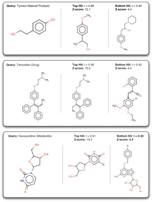
To test the similarity score statistical framework in practice, several example molecules, including natural products (Tyrosol), drug compounds (Tamoxifen), and metabolites (deoxyuridine) were queried against a random subset of ChemDB containing 1M compounds (Fig. 5). While the top scoring hits show a large degree of visual similarity to the queries as expected, the bottom hits also retain a certain degree of visual similarity and contain several common substructures. Also in line with the theoretical framework, the top hits have scores close to t=1.0, particularly for Tamoxifen and deoxyuridine, as predicted by the distribution of maximum scores f_max(t).

Fig. 5.

Example molecules queried against ChemDB. For each query, the given number of hits refers to the number of molecules with similarity scores above t=0.4. The top scoring hits are also shown along with the lowest scoring hits above t=0.4, and their corresponding Z-scores.

While a detailed understanding of the similarity score distribution underlying a chemical database can be useful, even for individual queries performed by hand, such understanding becomes essential for large-scale, high-throughput, computational studies, where manual inspection of all the hits is not feasible. Such studies are becoming routine in the areas of metabolomics, chemical genomics, systems biology and drug screening/discovery. In these areas, understanding the statistical properties of chemical similarity scores should be vitally important for identifying new molecules of interest, building effective computational screening pipelines, and furthering our understanding chemical space.

REFERENCES

- Ackley DH, et al. A learning algorithm for Boltzmann machines. Cogn. Sci. 1985;9:147–169. [Google Scholar]
- Altschul SF, et al. Gapped blast and psiblast: a new generation of protein database search programs. Nucleic Acids Res. 1997;25:3389–3402. doi: 10.1093/nar/25.17.3389. [DOI] [PMC free article] [PubMed] [Google Scholar]
- Baldi P, et al. Lossless compression of chemical fingerprints using integer entropy codes improves storage and retrieval. J. Chem. Inform. Model. 2007;47:2098–2109. doi: 10.1021/ci700200n. [DOI] [PMC free article] [PubMed] [Google Scholar]
- Bender A, et al. Similarity searching of chemical databases using atom environment descriptors (molprint 2d): Evaluation of performance. J. Chem. Inform. Model. 2004;44:1708–1718. doi: 10.1021/ci0498719. [DOI] [PubMed] [Google Scholar]
- Bohacek RS, et al. The art and practice of tructure-based drug design: a molecular modelling perspective. Med. Res. Rev. 1996;16:3–50. doi: 10.1002/(SICI)1098-1128(199601)16:1<3::AID-MED1>3.0.CO;2-6. [DOI] [PubMed] [Google Scholar]
- Cedilnik A, et al. The distribution of the ratio of jointly normal variables. Metodoloski Zveki. 2004;1:99–108. [Google Scholar]
- Chen J, et al. ChemDB: a public database of small molecules and related chemoinformatics resources. Bioinformatics. 2005;21:4133–4139. doi: 10.1093/bioinformatics/bti683. [DOI] [PubMed] [Google Scholar]
- Chen J, et al. ChemDB update-full text search and virtual chemical space. Bioinformatics. 2007;23:2348–2351. doi: 10.1093/bioinformatics/btm341. [DOI] [PubMed] [Google Scholar]
- Coles S. An Introduction to Statistical Modeling of Extreme Values. London: Springer-Verlag; 2001. [Google Scholar]
- Fligner MA, et al. A modification of the Jaccard/Tanimoto similarity index for diverse selection of chemical compounds using binary strings. Technometrics. 2002;44:110–119. [Google Scholar]
- Flower DR. On the properties of bit string-based measures of chemical similarity. J. Chem. Inform. Comput. Sci. 1998;38:379–386. [Google Scholar]
- Frey B. Graphical Models for Machine Learning and Digital Communicaiton. Cambridge, MA: MIT Press; 1998. [Google Scholar]
- Galambos J. The Asymptotic Theory of Extreme Order Statistics. New York: John Wiley; 1978. [Google Scholar]
- Hassan M, et al. Cheminformatics analysis and learning in a data pipelining environment. Mol. Divers. 2006;10:283–299. doi: 10.1007/s11030-006-9041-5. [DOI] [PubMed] [Google Scholar]
- Hert J, et al. Comparison of topological descriptors for similarity-based virtual screening using multiple bioactive reference structures. Org. Biomol. Chem. 2004;2:3256–3266. doi: 10.1039/B409865J. [DOI] [PubMed] [Google Scholar]
- Hinkley DV. On the ratio of two correlated normal random variables. Biometrika. 1969;56:635–639. [Google Scholar]
- Holliday JD, et al. Grouping of coefficients for the calculation of inter-molecular similarity and dissimilarity using 2d fragment bit-strings. Comb. Chem. High Throughput Screen. 2002;5:155–166. doi: 10.2174/1386207024607338. [DOI] [PubMed] [Google Scholar]
- Irwin JJ, Shoichet BK. ZINC–a free database of commercially available compounds for virtual screening. J. Chem. Inform. Comput. Sci. 2005;45:177–182. doi: 10.1021/ci049714. [DOI] [PMC free article] [PubMed] [Google Scholar]
- James CA, et al. Daylight Theory Manual. 2004 Available at http://www.daylight.com/dayhtml/doc/theory/theory.toc.html.
- Leach AR, Gillet VJ. An Introduction to Chemoinformatics. Dordrecht, The Netherlands: Springer; 2005. [Google Scholar]
- Leadbetter MR, et al. Extremems and Related Properties of Random Sequences and Series. New York: Springer-Verlag; 1983. [Google Scholar]
- Marsaglia G. Ratios of normal variables and rations of sums of uniform variables. J. Ameri. Stat. Assoc. 1965;60:193–204. [Google Scholar]
- Pham-Gia T, et al. Density of the ratio of two normal random variables and applications. Commun. Stat.-Theory Methods. 2006;35:1569–1591. [Google Scholar]
- Rouvray D. Definition and role of similarity concepts in the chemical and physical sciences. J. Chem. Inform. Comput. Sci. 1992;32:580–586. [Google Scholar]
- Swamidass S, Baldi P. Bounds and algorithms for exact searches of chemical fingerprints in linear and sub-linear time. J. Chem. Inform. Model. 2007;47:302–317. doi: 10.1021/ci600358f. [DOI] [PMC free article] [PubMed] [Google Scholar]
- Tversky A. Features of similarity. Psychol. Rev. 1977;84:327–352. [Google Scholar]
- Xue L, et al. Profile scaling increases the similarity search performance of molecular fingerprints containing numerical descriptors and structural keys. J. Chem. Inform. Comput. Sci. 2003;43:1218–1225. doi: 10.1021/ci030287u. [DOI] [PubMed] [Google Scholar]
- Xue L, et al. Similarity search profiling reveals effects of fingerprint scaling in virtual screening. J. Chem. Inform. Comput. Sci. 2004;44:2032–2039. doi: 10.1021/ci0400819. [DOI] [PubMed] [Google Scholar]