A coarse-grained potential for fold recognition and molecular dynamics simulations of proteins

Abstract

A coarse grained potential for protein simulations and fold ranking is presented. The potential is based on a two-point model of individual amino acids and a specific implementation of hydrogen bonding. Parameters are determined for distance dependent pair interactions, pseudo bonds, angles, and torsions. A scaling factor for a hydrogen bonding term is also determined. Iterative sampling for 4867 proteins reproduces distributions of internal coordinates and distances observed in the Protein Data Bank. The adjustment of the potential and re-sampling are in the spirit of the generalized ensemble approach. No native structure information (e.g. secondary structure) is used in the calculation of the potential, or in the simulation of a particular protein. The potential is subject to two tests: (i) simulations of 956 globular proteins in the neighborhood of their native folds (these proteins were not used in the training set), and (ii) discrimination between native and decoy structures for 2470 proteins with 305,000 decoys, and the “Decoys ‘R’ Us” dataset. In the first test, 58% of tested proteins stay within 5 Å from the native fold in Molecular Dynamics simulations of more than twenty nanoseconds using the new potential. The potential is also useful in differentiating between correct and approximate folds providing significant signal for structure prediction algorithms. Sampling with the potential consistently regenerates the distribution of distances and internal coordinates it learned. Nevertheless, during Molecular Dynamics simulations structures are found that reproduce the learned distributions but are far from the native fold.

Introduction

Hierarchical description of complex systems motivates the creation of coarse grained or reduced models with two goals in mind: (i) capture essential features of the system with simplified models that can be solved exactly (or almost exactly), and (ii) describe quantitatively properties of complex systems with a reduced representation computed from detailed experiment or theory. Examples for coarse grained models of type (i) are the HP model on a square lattice [1], or the Elastic Network Model for protein flexibility [2, 3]. Examples for type (ii) models are detailed folding simulations on lattices [4], or coarse description of membranes [5]. Approaches of type (ii) attempt to significantly reduce the computational cost and at the same time maintain a high level of accuracy that approaches the results of more detailed models.

The potential we describe in the present paper belongs to class (ii). Our aim was to develop an empirical force field with a reduced set of variables for physical simulations of proteins in the neighborhood of the native states. Simulations at the coarse level can be done more efficiently than atomically detailed calculations. Indeed, we illustrate in the present manuscript test simulations with accumulated time length of tens of microseconds that require only 12 hours on 500 computer cores. A nanosecond simulation of a medium size solvated protein (200 amino acids) can take a few days. The computational saving for simulations is about 3 orders of magnitude. We expect that equilibrium distributions generated by simulations with the designed potential will show characteristics of atomically detailed simulations. In parallel we require that the potential will recognize native folds of proteins as the lowest energy minimum when compared with an extensive set of “decoy” structures.

Our potential is purely empirical and the experimental observables which we use to fit the potential parameters are native structures of proteins determined by experimental techniques and deposited in the Protein Data Bank (PDB) [6]. These observables are clearly incomplete and a correct energy function should reproduce also the thermodynamics and kinetics of the system.

In the last twenty years many energy functions were estimated from empirical structures of proteins using the methodologies initiated by the following studies: inverse Boltzmann formula (statistical potentials) [7], memory associated Hamiltonians [8], Z score optimization [9], and Mathematical Programming [10]. Learning potentials from empirical structures should be contrasted with physically based energy functions. The usual design of a physical energy relies on experiments (and/or ab-initio calculations) on small model systems [11-13]. From a learning view-point, an advantage of physical potentials is the separation of types of input (the data to learn)) from types of output (the data to predict). On the other hand, potentials that are learned from empirical structures recognize correct folds with significantly less computational resources compared to physical energies, allowing for more extensive exploration of conformation space. The number of degrees of freedom is smaller by a factor between five and ten even without explicit solvent.

The approach described in this paper is an extension of the usual implementation of statistical potentials. We therefore start with a brief discussion of statistical potentials. After the introduction of statistical potentials by Miyazawa and Jernigan [7], a number of groups, including for example, Sippl [14], Skolnick et al. [15], Betancourt and Thirumalai [16], Bryant and Lawrence [17], Hinds and Levitt [18] and others more recently [19-22] continue to develop this concept and to examine the basic algorithm, functional form, and the data sets.

The basic concept of statistical potentials is similar in spirit to that of the potential of mean force [23] but important differences remain. Let the complete coordinate vector in continuous space representing the system be X, and the subset of coordinates that we use to describe the protein be, y_i=1,…,n, for example the set of backbone torsions or distances between amino acids. The number of reduced degrees of freedom is n, while the number of total number of degrees of freedom in the system is N. If the probability of a conformation, p(X), is known we can determine the probability of a variable of interest, y_i, by direct integration p(y_i)= ∫ P(X)δ(y_i− ȳ_i(X))dX. The delta function matches the value y_i with the function of the canonical coordinates ȳ_i(X). If the probability P(X) obeys Boltzmann statistics (P(X)∝ exp[−βU(X)], U(X) is the potential energy, and β is the inverse temperature) then the probability p(y_i) is related to a potential of mean force (PMF), $V_i\left(y_i\right)=-\frac{1}{\beta }\text{log}\left(p\left(y_i\right)\right)$.

The first assumption made in the derivation of Statistical Potentials (SP) is that the Protein Data Bank (PDB) provides a Boltzmann sample of conformations, therefore a PMF can be estimated from the observed frequencies of certain degrees of freedom $V_i\left(y_i\right)=-\frac{1}{\beta }\text{log}\left(f\left(y_i\right)\right)$ [7].

The second assumption made in the calculations of SP is the representation of the total potential as a sum of PMF terms. An “energy” of the system is written as U(y₁, y₂,…, y_n)= V₁(y₁)+ V₂(y₂)+ …+V_n(y_n).

The problem with this assumption is easy to illustrate using the definition of the PMF. The “energy” in the subspace of y_i=1,…,n is used to sample conformations in the full coordinate space of the protein X. The sampling is in the canonical ensemble with β for inverse temperature and for all degrees of freedom X:

$$p\left(y_i\right)=\int exp\left[-\beta \left(V_1\left(y_1\right)+\dots +V_i\left(y_i\right)+\dots +V_n\left(y_n\right)\right)\right]\cdot \delta \left(y_i-{\overline{y}}_i\left(X\right)\right)J\left(Y,X\right)d\Gamma \prod _{j}d{y}_j,$$

where we plugged in the integral the usual form of the statistical potential, dΓ is a volume element of the remaining coordinates not in .y_i.'s, and J(Y, X) is the Jacobian of the transformation from X to Y. Note that X and Y are not of the same dimension and Γ denotes the remaining degrees of freedom.

Instead of the statistical potential we can write a new effective energy that is used in the sampling $V_{\mathrm{eff}}\left(y_1,\dots ,y_n\right)=\text{∑}_i{V}_i\left(y_i\right)-\left(1/\beta \right)\text{log}\left[J\left(X,Y\right)\right]$. If the Jacobian was a constant then we would trivially recover the probability p(y_i) ∝ exp(−βV(y_i)) that we started with. However, for most degrees of freedom used in statistical potentials (e.g. distances) this is not the case. We can still seek an effective potential V* (y_i) that will make the desired definition of the mean force potential to hold, i.e. $\overline{p}\left(y_i\right)\propto \int \text{exp}\left(-\beta \text{∑}_i{V}_i^{\ast }\left(y_i\right)+\text{log}\left(J\left(X,Y\right)\right)\right)\delta \left(y_i-{\overline{y}}_i\left(X\right)\right)d\Gamma \text{∏}_{j}d{y}_j$ and at the same time p̄(y_i) is equal to the PDB distribution p(y_i). A statistical potential used “as is” will not reproduce the PDB distribution if it is implemented in an algorithm that generates the canonical distribution. Note that the potential V* (y_i) and the distribution p(y_i) are no longer related by the inverse Boltzmann relation. The algorithm proposed in the present paper attempts to generate such a V* (y_i).

Besides the basic difference between PMF and SP pointed above, writing the overall potential as a sum of PMFs introduces additional approximations. The first is the factorization of the overall probability to a product of probabilities. It suggests lack of correlations between the y_i's. The use of multiple internal coordinate probabilities [24-26] p(y_iy_j) addresses some of the concerns. However the choice of correlations to focus on is not trivial and acquiring appropriate statistics for these higher order interaction terms is another challenge. The second approximation is the use of types. It is not obvious that probability distribution of type α (e.g. a contact between phenylalanine and valine) will be the same in a different environment (e.g. hydrophobic or polar medium).

SP most frequently aim at the fold recognition problem; i.e., given a set of plausible structures that are all protein-like, how to choose a configuration that is the closest to the native fold. It typically does not address the problem of direct and extensive sampling of configuration space with a potential according to a pre-determined weight (e.g. canonical). In the present manuscript we generate a potential that is consistent with both (MD simulations and fold recognition). Not surprisingly new problems emerge. One practical problem is that the sampling of coordinate space in the PDB is incomplete. As a result MD simulations with straightforward statistical potentials do not produce protein-like conformations.

The problem of generating a single potential, which is optimal for the task of fold recognition and of MD simulations, can be solved by additional potential terms that take care of interactions poorly sampled in the PDB. The combination of the statistical potential and the new terms is not obvious. Once these terms are added to “traditional” statistical potentials the simulations with the adjusted energy function no longer (necessarily) reproduce the distributions of the y_i's extracted from the PDB. The present manuscript is addressing this particular problem by adopting an algorithm from condensed phase simulations which is a variant of the generalized ensemble approach [27]. It generates iteratively a potential consistent with the PDB distributions of internal coordinates and the supplements discussed above.

The resulting potential is significantly more complex than the usual form of statistical potentials. It is also continuous and differentiable. We emphasize that even with these advances the paper does not address the two basic approximations of statistical potentials (factorization of the probability and transferability of parameters). It is therefore not surprising that significant deviations from native folds are still observed in simulations for a significant number of proteins, even if the design requirements are satisfied. Despite the drawbacks, the performance we obtain with the final form of the potential is adequate for the usual fold recognition (and it was used in CASP8 http://predictioncenter.org/casp8/index.cgi), and also for Molecular Dynamics simulations. Another continuous and differentiable potential that learns its parameters from the PDB with a different technique and can be used for energy minimization and simulations was introduced recently [28]. Bridging potential parameters from small molecule data to macromolecular modeling was also pursued recently by Z score optimization [29]. These potentials are however designed for all atom models.

Potential functional form

In this section we present the functional form and the parameterization of a new coarse grained potential which we call FREADY (a potential for Fold REcognition And DYnamics). The starting functional form and parameterization of the potential were motivated by the simple physical model of the group of Thirumalai [30] and its enhancements by the group of Head-Gordon [31, 32]. However, as we look in more detail into the conformation data available in the Protein Data Bank and examine structures generated by Molecular Dynamics (MD) simulations (using coarse grained potentials), a significantly more complex form becomes necessary.

The number of degrees of freedom in the complex form remains relatively small, only two points per amino acid are used - the position of the Cα atom and the side chain center of mass (CM). It was also decided to keep the functional form independent of any information about the native structure (e.g. secondary structure or native contacts); thus enabling unbiased dynamical studies of biophysical processes where the information about the native conformation is not available or well defined (e.g. large conformational transitions).

The potential employs the functional form (1.1) that includes bond, angular, and torsional terms as well as non-bonded interaction and explicit hydrogen bonding. Solvent is treated implicitly since the parameters of the potential are learnt from statistics of solvated protein. By insisting that solvent induced structures (most structures in the PDB are reasonably well solvated) are reproduced in the simulations we incorporate some solvent effects.

$$\begin{array}{l}\begin{array}{c}U(X)=\text{∑}_{i\in \mathrm{bonds}}{U}_B(r_i,{\tau }_{Bi})+\text{∑}_{i\in \mathrm{angles}}{U}_A({\theta }_i,{\tau }_{Ai})+\text{∑}_{i\in \mathrm{torsions}}{U}_T({\varphi }_i,{\tau }_{\varphi i})\\ +\text{∑}_{i,j>i}{U}_{NB}(r_{ij},{\tau }_i,{\tau }_j)+\text{∑}_{i\in \mathrm{dipole\; centers}}{U}_{HB}(i)\end{array}\end{array}$$ (1.1)

We denote by τ the type of interactions (for example atom type, or the type of a bond between two atoms). Typically, bond and angle interactions in other force fields (atomic or coarse grained) are modeled by quadratic terms with a single minimum; however these functions do not give acceptable fits to the statistics of bond lengths and angles we extract from the PDB structures (Figure 1) and later from MD. The reason is that the internal degrees of freedom of side chains and backbone that are removed in the coarse representation have internal structure with multiple stable states that is reflected in multiple minima of the coarse variables. This observation is especially true for covalent terms that include a side chain atom but is also correct for angles of three sequential backbone atoms (Cα). Therefore, the bond energy as well as the angle energy terms of FREADY, are described with a single, a double, or a triple well potential (see Eq. (1.2) and (1.3)). The multiple well potentials we consider in this work are

Figure 1.

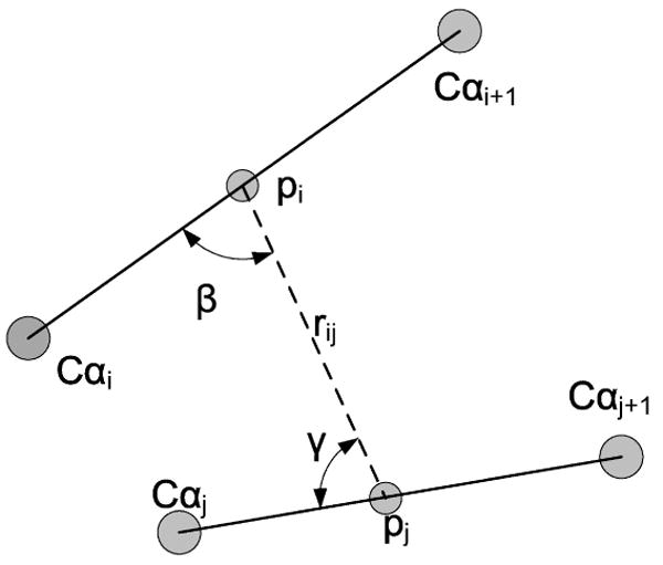
Description of terms entering the calculation of the backbone hydrogen bonding term U_HB(i, j). The angle α_ij is defined as an angle between the bonds C_αi − _αi+1 and C_αj − _αj+1.

$$U_{B/A}(x,\tau )=\{\begin{array}{ll}{k}_{\tau }{(x-x_{\tau })}^2& \text{if}\tau \in \text{terms with a single well}\\ C\left(k_{\tau 1}{(x-x_{\tau 1})}^2,k_{\tau 2}{(x-x_{\tau 2})}^2+{\alpha }_{\tau },{\beta }_{\tau }\right)& \text{if}\tau \in \text{terms with a double well}\\ C\left\{C\left(k_{\tau 1}{(x-x_{\tau 1})}^2,k_{\tau 2}{(x-x_{\tau 2})}^2+{\alpha }_{\tau },{\beta }_{\tau }\right),k_{\tau 3}{(x-x_{\tau 3})}^2+{{\alpha }^{\prime }}_{\tau },{{\beta }^{\prime }}_{\tau }\right\}& \text{if}\tau \in \text{terms with a single well}\end{array}$$ (1.2)

$$C(U_1,U_2,\beta )=\frac{1}{2}\left(U_1+U_2-\sqrt{{\left(U_1-U_2\right)}^2+{\beta }^2}\right),$$ (1.3)

where x denotes a bond length or an angle size and all variables with τ in the subscript are potential parameters to be determined. The parameters x_τ are equilibrium positions, k_τ are force constants, α_τ are relative energy differences between the different minima, and β_τ are determining the barrier height between two wells. The coupling function C(U₁,U₂,β) joins the two energy functions U₁ and U₂ as in empirical valence bond theory [33], a form that was used in another coarse grained model [34, 35]. Triple well terms require multiple parameters α and β.

The current model has 22 different types of bonds and 58 different types of angles. There are 19 different bonds between Cα and CM particles for each of the different amino acid (GLY does not have a CM particle), one bond type for the typical Cα-Cα backbone bond, one for a bond between Cα of a proline in a cis-isomer and a preceding Cα atom. The last bond type is for modeling the disulfide bridges between cysteine residues.

The 58 angle types are built from the following three templates Cα_i-1-Cα_i-Cα_i+1, CM_i-Cα_i-Cα_i-1, and CM_i-Cα_i-Cα_i+1 for each different type of a central (Cα_i) atom with the exception of GLY. The 20 types of angle templates Cα_i-1-Cα_i-Cα_i+1 are all very similar and could be reduced to a single backbone angle type. Since subtle differences may have remained we did not merge all these terms in the first version of the potential.

The torsional terms U_T(φ,τ_φ) take as input an angle φ and a type of the torsional angle τ_φ. The torsional term is modeled as the following sum of cosine and sine terms:

$$U_T\left(\varphi ,{\tau }_{\varphi }\right)=\text{∑}_{n=1}^5{C}_{\tau ,n}cos(n\varphi )+S_{\tau ,n}sin(n\varphi )$$ (1.4)

We have used five expansion terms for the periodic function. This number of terms is probably unnecessary, however, in the present version of the potential they do not harm. It is still possible that subtle effects are captured by the high order terms and therefore we left these terms “as are” and did not attempt to simplify them further. There are almost 4 · 20² different types of torsional/dihedral angles: A torsion (the angle between two planes) is defined by four points. All torsions in our model are along Cα_i-Cα_i+1 backbone bonds (we do not consider torsions related to CYS-CYS bonds). The type of a torsional interaction, τ_φ, is determined by the residue types of the central Cα pairs and by the particle types (Cα or CM) of the two remaining points. For a given Cα pair there can be up to four different dihedral angles present (Cα_i-1-Cα_i-Cα_i+1-Cα_i+2, CM_i-Cα_i-Cα_i+1-Cα_i+2, Cα_i-1-Cα_i-Cα_i+1-CM_i+1, and CM_i-Cα_i-Cα_i+1-CM_i+1). The number of different torsional types is not exactly 4 · 20² since glycine does not have a side chain.

The function U_NB(r,τ₁,τ₂), describes non-bonded interactions where τ₁, τ₂ are the types of the interacting particles and r is the distance between them. There are 39 different particles considered for non-bonded interactions (20 Cα atoms and 19 CM particles). Thus we have $\frac{39\cdot 40}{2}$ types of non-bonded interactions in the system. The function U_NB(r,τ₁,τ₂) is continuous and differentiable to the first order and is defined below.

$$U_{NB}(r,{\tau }_1,{\tau }_2)=\{\begin{array}{ll}{U}_{NB}^0(r)+A_{{\tau }_1{\tau }_2}{r}^{-6}+B_{{\tau }_1{\tau }_2}{r}^{-2}+C_{{\tau }_1{\tau }_2}& \text{if}r<4.2\mathring{\text{A}}\\ U_{NB}^0(r)+\text{∑}_{i=0}^9{a}_{{\tau }_1{\tau }_{2}i}{r}^i& \text{if}r\in \langle 4.2\mathring{\text{A}},13.5\mathring{\text{A}}\rangle \\ 0& \text{if}r>13.5\mathring{\text{A}}\end{array}$$ (1.5)

$$U_{NB}^0(r)=\{\begin{array}{ll}0.6\cdot {10}^7{r}^{-12}-3\cdot {10}^3{r}^{-6}& \text{between CM}‐\text{CM particles}\\ 0.6\cdot {10}^6{r}^{-12}& \text{otherwise}\end{array}$$ (1.6)

We do not consider a pair of particles for non-bonded interactions if they are separated by one or two bonds; if they are separated by three bonds (1-4 interaction) we scale the non-bonded interaction down by a factor f₁₄. S-S bonds between CYS residues are not considered for these exceptions. If a scaling factor f₁₄ = 1 is used the non-bonded energy distorts the local geometry when CM_i and CM_i+1 are a strongly repulsive pair. At the other limit, if f₁₄ = 0, some pairs of neighboring sidechains may overlap. The value of f₁₄ was set to 0.3 after some experimentation and was found to reproduce well the local structure.

Backbone hydrogen bonding potential between residues i and j,U_HB(i, j), is based on the model developed by Liwo and coworkers [36, 37]. These hydrogen bonds are modeled by dipole interactions between the peptide centers which are implicitly assumed to be located in the centers of Cα-Cα bonds. The explicit functional form of U_HB(i, j) is given below

$$\begin{array}{l}{U}_{HB}(i,j)=\frac{A_{{\tau }_i{\tau }_j}}{r_{ij}^3}{f}_{ij}-\frac{B_{{\tau }_i{\tau }_j}}{r_{ij}^6}\left[4+f_{ij}^2-g_{ij}\right]+{\epsilon }_{{\tau }_i{\tau }_j}\left[q_{ij}^{12}-2q_{ij}^6\right]\\ q_{ij}=\frac{r_{{\tau }_i{\tau }_j}^0}{r_{ij}}{f}_{ij}=cos{\alpha }_{ij}-3cos{\beta }_{ij}cos{\gamma }_{ij}{g}_{ij}=3({cos}^2{\beta }_{ij}+{cos}^2{\gamma }_{ij})\end{array},$$ (1.7)

where r_ij, α_ij, β_ij, and γ_ij are the coordinates that determine the geometry of a hydrogen bond (Figure 1). There are two types of peptide centers (τ_i ∈ {1,2}) defined in this work similarly to reference [37]: a usual peptide bond and a proline-type peptide bond. The interaction parameters to be determined are $r_{{\tau }_i{\tau }_j}^0$, A_τiτj, B_τiτj, and ε_τiτj. Eq. (1.7) is derived in [37] by Boltzmann averaging over torsional degrees of freedom of the two interacting dipoles. Our initial attempt to model backbone hydrogen bonding by $\text{∑}_{i,j}{U}_{HB}(i,j)$ follows UNRES [36, 37]. However, with other terms at hand, simulations with the UNRES potential generate conformations that are often too compact and contain unnatural hydrogen bonding patterns. Another observation was that typically each residue contributed to the sum $\text{∑}_{i,j}{U}_{HB}(i,j)$ by 1 to 5 partners, five hydrogen bonds per residue are too many compared to the typical saturation number of about two that we observed in the PDB. To reduce over bonding of the hydrogen bonds within the context of FREADY potential, we retain at most the two strongest interactions described by Eq. (1.7) per amino acid. The hydrogen bond energy of a site i is determined as follows. The energies of all the candidates j for a hydrogen bond with i, U_HB(i, j), are sorted and the lowest energy, $H{b}_{ij}^{(\text{min})}$ is kept. We then examine the possibility of having two (lowest energy) hydrogen bonds to the site i. The energy of the two hydrogen bonds depends on their relative orientation φ_jik, $H{b}_{\mathrm{ijk}}^{\left(\text{min}\right)}=\text{min}\left(U_{HB}\left(i,j\right)+U_{HB}\left(i,k\right)\right)\cdot F\left(-cos\left({\varphi }_{\mathrm{jik}}\right)\right)$, where φ_jik is the angle between the dipole centers j, i, and k.

$$F(x)=\{\begin{array}{cc}\hfill 1\hfill & \text{if}x>0.9\hfill \\ \hfill \left(x-0.3\right)/0.6\hfill & \text{if}x\in \left[0.3,0.9\right]\hfill \\ \hfill 0\hfill & \text{if}x<0.3\hfill \end{array}$$

The optimal single bond energy is then compared to the optimal two-hydrogen-bond energy and the option with the lowest energy is used

$$U_{HB}(i)=\text{min}\left[H{b}_{ij}^{\left(\text{min}\right)},H{b}_{\mathrm{ijk}}^{\left(\text{min}\right)}\right].$$ (1.8)

Learning the potential parameters

As discussed in the introduction the most common approach to derive parameters of a statistical potential is based on the assumption of mutual independence of different interactions in the protein. Based on statistics collected from experimental structures the potential function along a degree of freedom q is obtained by Boltzmann inversion formula

$$U(q)=-k_{B}Tln\left(\frac{P_{\mathrm{native}}(q)}{P_{\mathrm{reference}}(q)}\right),$$ (1.9)

where k_B is the Boltzmann constant, T is the temperature (300 K), and P_native (q), P_reference(q) are probability distributions of a variable q in the experimentally solved dataset and an expected probability distribution of q (also known as the reference state). Examples for reference states are (i) a state of no interactions between amino acids (unfolded protein), and (ii) a state of random interaction between the amino acids. A proper choice of the reference state was a topic of much discussion in the literature [16, 38]. The complete potential for a particular protein is given by a sum of U(q) terms: ${\overline{U}}_{\mathrm{total}}\left(q_1,\dots ,q_l\right)=\text{∑}_{i=1}^{l}U\left(q_i\right)$. This functional form assumes that the total probability of finding these variables factors into a product of probabilities of individual terms.

We bridge the learning of potentials for fold recognition and potentials for Molecular Dynamics simulations by iterative procedure to recover the native distributions of relevant degrees of freedom P_native(q_j), where j is an index that goes through types considered in Eq. (1.1) (e.g. distance between Cα particles of ALA and THR residues). Before the first iteration, the training set of native structures is used to calculate P_native(q_j) and a zero-order potential Ū₀(q₁, …,q₁) is chosen. The particular choice of Ū₀(q) is not important and any reasonable initial guess is corrected in the following learning iterations. The potential Ū_i(q) is then used to initiate long Molecular Dynamics trajectories in the CG model producing canonical distribution of structures at room temperature (300 K) consistent with Ū_i(q). These simulations are run for 600 picoseconds (with a time step of 3 fs) and for all proteins (4867) in the training set. Probability distributions P_i(q_j) of bond lengths, angles, torsions, pairwise particle distances and hydrogen bond lengths are collected from the final structures of simulated trajectories. However, as discussed in the introduction, canonical sampling with statistical potentials does not reproduce the PDB distributions because of the Jacobian coupling. An attempt to fix this problem is to consider the ratio of the sampled and of the native distributions. The logarithm of the ratio of these probabilities will be added to the potential to initiate a new iteration (new Molecular Dynamics trajectories with the fixed potential). The formula for the adjustment (following Reith and co-workers [39] and [40]) is

$$U_{i+1}(q)=U_i(q)+k_{B}Tln\left(\frac{P_i(q)}{P_{\mathrm{native}}(q)}\right).$$ (1.10)

We reiterated the calculations of the potential and Molecular Dynamics simulations a number of times until the correction to the potential parameters was negligible, in practice this happens in about 20 iterations. It is similar in spirit to a generalized ensemble approach that was used extensively by others (see for instance [41]). Reith and co-workers proposed this procedure to derive coarse grained potentials for polymers. Atomically detailed simulations were used in their work to define P_native(q_j). Instead of running expensive all-atom MD simulations on the whole training set we infer P_native(q_j) from the structures deposited in PDB.

It is important to emphasize the difference of equation (1.10) from the usual statistical potential approach [7] which is a one step calculation from probability to potential. The iterative form of equation (1.10) allows us to add external terms (external to the probabilities determined from the PDB) and use the iterations to merge the different terms such that the original probabilities will be recovered in the canonical sampling. Such a potential refinement scheme is new and is not part of the “traditional” statistical potential approach. The final distributions P(q_j) that we obtain are not identically equal to the native PDB distributions. However, the deviations are within the usual statistical errors of this type of calculation (Figures 2 and 4) and are due to the discrete representation of the distributions and the finite size of the training set.

Figure 2.

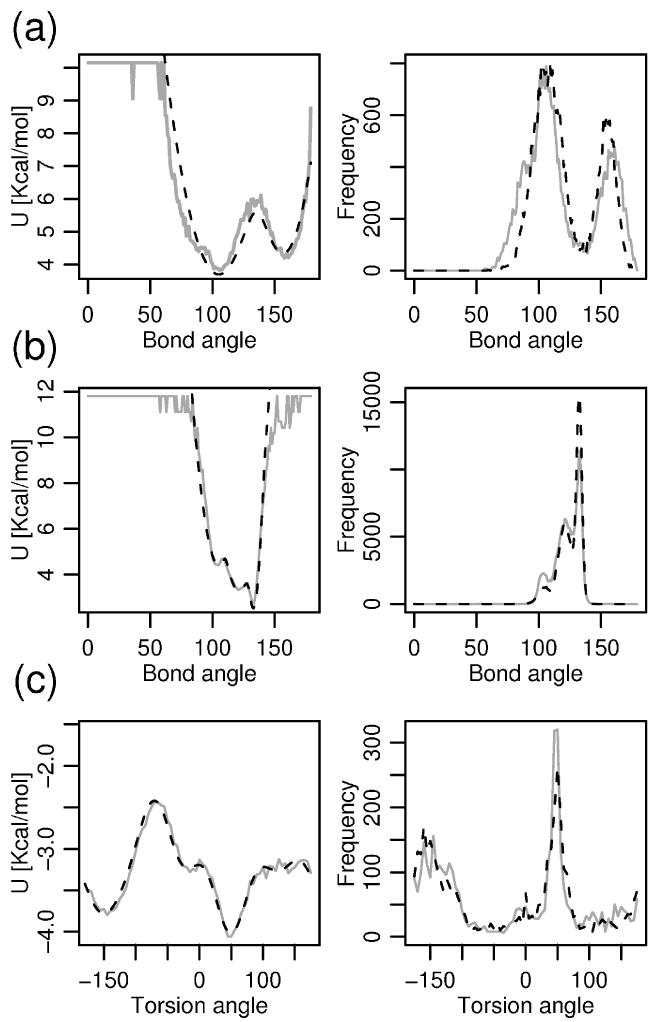
(a) left: Fit of the angle interaction term defined by Cα _i-1, Cα _i,CM_i for i-th residue being a TRP obtained by Boltzmann's inversion of the native distribution (gray) and the analytical fit to a double-well function (black, dashed). right: Comparison of distributions for this type of angles seen in the native structures (gray) and in the MD simulations driven by FREADY (black, dashed). (b) same as in (a), only for the central residue being VAL. The angle is of triple-well character in this case. (c) left: Fit by Discrete Fourier Transform (black, dashed) to the final version of the torsion potential (gray) defined by four consecutive Cα particles (for central two residues being TYR, ASN) right: Comparison of this torsion angle distribution in the native structures (gray) and in the MD simulations (black, dashed) for this dihedral angle type.

Figure 4.

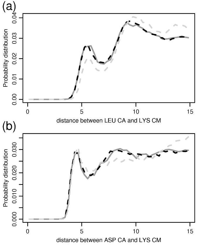
Radial distribution functions between pair of particles (a) LEU-Cα and LYS-CM (b) ASP-Cα and LYS-CM. The solid line corresponds to the distribution in the native structures, gray-dashed line depicts the distribution obtained after the first iteration of the training, and the black-dashed one stands for the distribution seen in the structures simulated by the final version of FREADY.

Nevertheless, one must keep in mind that even with the iterations the potential is approximate. First (as discussed above) the factorization is an approximate procedure and only a general P(q₁,…q_l) is exact. Second, it is assumed that the potential is transferable, i.e. that we can have one coarse grained potential to describe many proteins. Third, we assume that the iterative process of running Molecular Dynamics trajectories and adjusting the potential as described above converges to a stable solution (there is no proof of convergence). With the above mentioned approximations, it is perhaps no surprise that the procedure we finally adopt to compute all the potential parameters involved considerable heuristic, and that the resulting potential is not perfect: (i) it does not recognize native folds as the lowest energy in all cases, and (ii) MD simulations sampled with significant probability (for some proteins) structures that are far from the native fold.

As a training set, we used a set of PDB protein structures that forms the prediction database for our modeling program LOOPP (http://www.loopp.org, for a recent publication see [42]). It includes 9513 native structures that have at most 70% sequence identity between any two proteins in the set. This is higher sequence similarity than similarity used in other studies of statistical potential (about 20%). Our data provides reasonably dense sampling in sequence space. At least for fold recognition (after all, we wish to predict protein structure from a sequence) we argue that folds with larger sequence capacity (the number of sequences that are compatible with a given fold [43]) should have a higher weight than folds that capture only a few sequences. This weight might be lost if the selection emphasizes structural diversity instead of sequence variations. Another (pragmatic) reason that led us to broaden the set of structures and sequences is that of statistics. We need more proteins in order to obtain reliable statistics to fit our complex differentiable interaction terms (e.g. we need to sample at least 100 times every pair of neighboring residues along the backbone to fit reliably each torsional interaction).

The training set is further refined by removing membrane proteins [44, 45] and proteins complexed with polynucleotides [46]. All occurrences of selenomethionines (MSE) were replaced by regular MET residues and pyroglutamic acids (PCAs) were removed from the C-terminals. Proteins that contain other non-standard amino acids were removed from the training set. We used structures that correspond to the biological molecules (remarks BIOMT 350 in the PDB files) rather than the units determined by crystallography. In the training process we limited ourselves to globular proteins, therefore proteins with radius of gyration 15% larger than expected were not considered. The formula for expected radius of gyration of globular proteins $Rg=0.395N^{\stackrel{3}{}/\underset{5}{}}+7.257$ was taken from [47, 48]. Lastly, since MD simulations for larger proteins take longer time only proteins with at most 750 residues are used in the training process. The final training set contains 4867 proteins. All MD simulations were performed in the MOIL molecular modeling package [49] (http://clsb.ices.utexas.edu/prebuilt/) and the final version of FREADY is fully integrated with other functionalities of the package such as energy minimization or visualization. MD calculations conducted with FREADY potential are about 10³ faster than an all-atom simulation in explicit solvation. The converged set of FREADY potential parameters can be found in the file moil.mop/CG.PROP of the MOIL distribution package or is also available in an extended form in the tar file http://clsb.ices.utexas.edu/research/group/fready.tgz.

In practice, distributions P_i(q) and P_native(q) are represented as discrete sets of bins. Bin sizes used in this work are 0.1 Å, 1°, 3°, 0.3 Å, and 0.1 Å for bond, angle, torsion, non-bonded, and hydrogen-bonding terms respectively. The discrete descriptions of U_i+1(q) are then fitted by continuous functions described in Eq. (1.2) - (1.8). Fitting of bond and angle parameters has been performed manually, since the convergence is reached after one or two iterations. Torsional terms are fitted in a straightforward manner by the Discrete Fourier Transform algorithm.

The parameters A_τiτj, B_τiτj, and ε_τiτj of the backbone hydrogen bonding term U_HB(i, j) are not optimized independently in this work, but their ratios are taken from [50] where they were optimized by fitting restricted free energy surfaces of UNRES model to those obtained from all atom simulations. Only the overall multiplicative factor of these energy constants and the parameters $r_{{\tau }_i{\tau }_j}^0$ are optimized so that the distribution of hydrogen bond lengths seen in MD simulation in the FREADY model matches those seen in the experimental native structures. The resulting distributions of angles describing the geometry of hydrogen bonds (α, β, γ) agree with corresponding native distributions (even the parameters A_τiτj, B_τiτj were optimized only relatively based on the hydrogen bonds length distribution).

We can use the hydrogen bonding functional form developed for UNRES since the coarsening in FREADY is similar to that in UNRES model. UNRES, same as FREADY, represents each residue by two beads. A difference is that in UNRES positions of the peptide centers are considered explicitly and positions of Cα atoms are implicitly reconstructed. In FREADY, we explicitly model the Cα particles and the centers of the hydrogen bonding groups are assumed to be in the center of the Cα-Cα bonds. Conceptually UNRES relies on chemical physics principles, while the main drive of the FREADY model is the requirement that hydrogen bond distribution of MD simulations will mimic the hydrogen bond distribution observed in statistics of experimentally determined protein structures. The use of a hydrogen bond term is also a nice illustration of mixing different potential terms (from different sources) with the iterative sampling.

Fitting of U_NB(r, τ₁, τ₂) is more complex and has been fully automated. In order to speed up convergence of our iterative algorithm it is a good idea to obtain a reasonable zero order guess for non bonded interactions. The zero order guess we have used is a Lennard Jones like potential between all pairs of CM particles and a repulsion r⁻¹² term between all other particles which are described by $U_{NB}^0(r)$ in Eq. (1.6). For sake of simplicity, $U_{NB}^0(r)$ does not depend on interacting residues' types and residue dependent features of the non-bonded term are recruited throughout the iterative learning process. The three adjustable parameters of $U_{NB}^0(r)$ were selected such that the average radius of gyration is conserved after 600 ps long MD simulation for the structures in the training set.

For numerical reasons the functions U_NB(r,τ₁,τ₂) are not fitted along the whole range of distances at once. The non bonded interactions are constructed as piecewise continuous and differentiable (to the first order) terms. The distances in range r∈〈4.2Å,13.5Å〉 are fitted by least squares (LS) algorithm to nine degree polynomials. The optimization is constrained such that the function U_NB(r,τ₁,τ₂) and its first derivative vanish at r = 13.5Å. The parameters A_τiτj, B_τiτj, and C_τiτj (from Eq. (1.5)) of the target functions are fitted against the distributions at distances smaller than 4.2 Å with the constraints that U_NB(r,τ₁,τ₂) has continuous first derivative at r = 4.2Å. The function splitting at 4.2 Å was motivated by steep characteristics of U_NB(r,τ₁,τ₂) at shorter distances and by rather smooth behavior of the non-bonded potential at larger separation.

Results

The iterative algorithm described in the previous section converged to a fixed set of parameters for the FREADY potential after about 20 iterations. Covalent local interaction terms such as bond lengths converge more rapidly and stabilize after a few (up to three) iterations. Figure 2 shows typical converged angular and torsional interactions. Comparisons of the native distributions to those obtained from the final training iteration are also shown. In Figure 3 we illustrate how a non-bonded interaction term evolves during the training process and Figure 4 illustrates how the radial distribution functions between these pairs of residues evolved from the initial to the final iteration. Overall individual distributions of the variables extracted from the PDB are accurately represented by the converged distributions of the final iteration. The small deviations from the PDB distribution that are observed in Figure 4 are typical.

Figure 3.

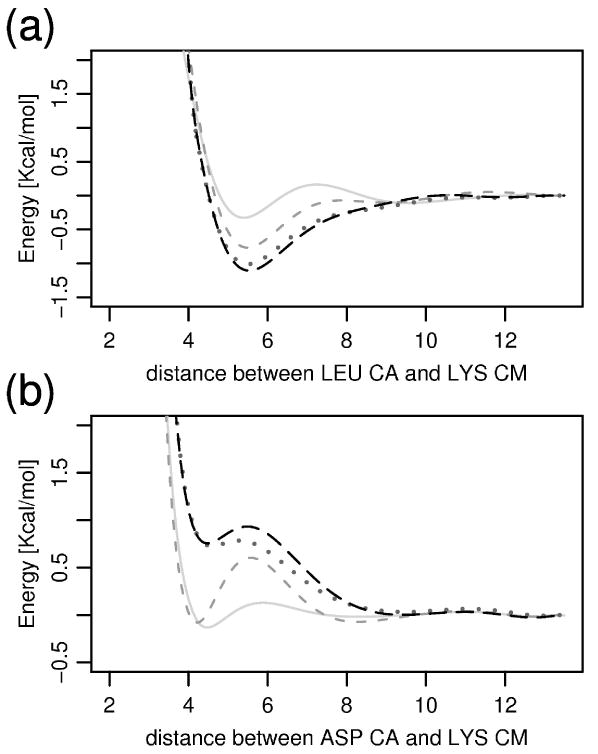
Iterative adjustments to the non-bonded interaction term between (a) LEU particle Cα and LYS particle CM; (b) ASP particle Cα and LYS particle CM. The interactions are evolving during the training in the order gray-solid (1. iteration), gray-dashed (3.iteration), dotted (11. iteration), and black-dashed (the final, 20^th, iteration).

The quality of the final set of FREADY parameters was verified by two different tests: a) a stability test of the native protein conformations during MD simulations and b) a decoy recognition task. The stability of native conformations in FREADY potential was tested on native structures of proteins independent of the training set. The set used for the iterative training was based on the non-redundant set of protein structures covering the shapes available in PDB as of 6/28/2005. The test set for FREADY potential includes non-redundant representation of the protein structures deposited to the PDB between 6/28/2005 and 6/13/2006 [42].

The test set was filtered, as was done for the training set. We remove membrane proteins, RNA/DNA complexes, and PCAs (pyroglutamic acids). Group type MSEs (selenomethionines) are replaced by MET. Proteins with other non-standard amino acids were removed. Only proteins with typical radius of gyration were kept). Further on, we reduced the test set to single chain proteins without any breaks in the backbone and limited the size of each protein to up to 500 residues. After all these constraints are met the test set consists of 956 native structures. A 21 ns MD simulation of each structure from the test set (driven by FREADY potential function) was performed. Every simulation begins from the native conformation by a short (200 steps) conjugate gradient minimization. The simulations are initiated with 300 ps linear heating from 1 K to 300 K followed by 20.7 ns constant temperature simulation (controlled by velocity scaling).

Figure 5 shows a distribution of the RMSD of the final structure of each MD simulation and the corresponding native conformation. Similarly Figure 6 shows distribution of the TM-score [51], which is measure of structural similarity that scales between 0 and 1. It is calculated as

Figure 5.

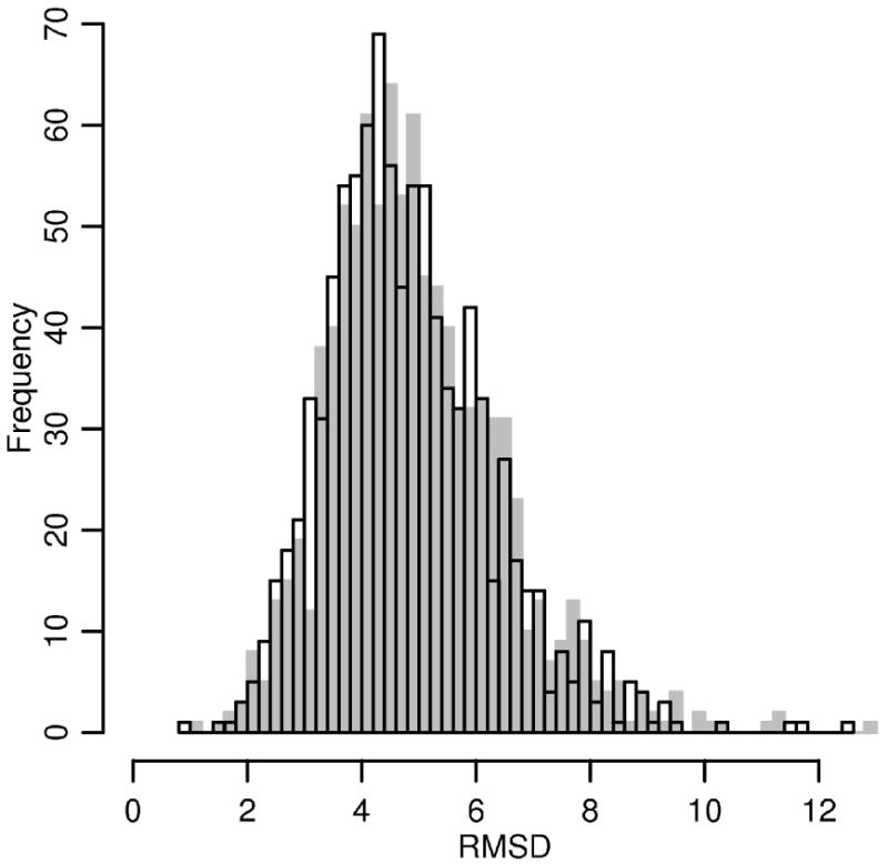
The distribution of RMSD from the native fold after 10 ns (gray) or 21 ns (black, transparent) long MD simulation initiated from the native conformation.

Figure 6.

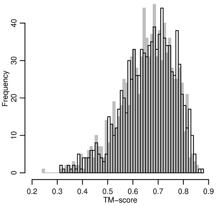
The distribution of TM-score between the native fold and structures obtained by 10 ns (gray) or 21 ns long (black, transparent) long MD simulation starting from the native conformation.

$$\text{TM}-\text{score}=\text{max}\left[\frac{1}{L}\text{∑}_{i=1}^L\frac{1}{1+{\left(\frac{d_i}{d_0}\right)}^2}\right],$$ (1.11)

where L is the protein length, d_i is the distance between i-th pair of residues, $d_0=1.24\sqrt[3]{L-15}-1.8$ is a distance scale, and maximum is taken over all structural superpositions. In contrast to RMSD the TM score can capture local similarities while the RMSD is sensitive to overall changes and to outliers. TM-score is calculated by an algorithm described in [51] and available from http://zhang.bioinformatics.ku.edu/TM-score/. The mean RMSD and TM-score against the native structures after 21 ns MD simulation are 4.95Å or 0.65, respectively. Figures 5 and 6 also show the distributions after 10 ns of MD. Only minor differences between the final distributions are observed. This observation suggests that most of the structures in the test set reach equilibrium after 10 ns.

The equilibrated distributions of internal degrees of freedom after 21 ns of MD are in good agreement with the distributions obtained from the native folds. Nevertheless, as shown on Figure 5 and 6, even when the target distributions of internal coordinates are preserved there are structures that diverge significantly from the native fold (RMSD larger than 10 Å or TM-score less than 0.4). This implies that the functional form of the potential chosen in the present manuscript (i.e. sum of local, pairwise terms and backbone HB) is not sufficient to fix the average structure in the neighborhood of the native fold during room temperature simulations.

In Figure 7 we show results for three representative medium sized structures. Two of these proteins (1ido, 1a3k) remain relatively close to the native structure (RMSD of 2.33 Å and 3.42 Å). The third protein shown (1ge6) is an example in which the MD simulation drives the structure away from the native structure (9.87 Å). Figure 8 shows a comparison of mean square displacements of Cα particles during the last 10 ns of the test simulation with experimental crystallographic B-factors. The mean square displacements are in weak agreement with the experimental values. The location of the large fluctuations along the sequence seems to agree with experiment, but not the amplitudes. There are several residues in loop regions and close to either N or C terminals that have significantly higher displacements than those implied by B-factors. The same figure also shows that many of these overly-flexible parts of the structures are predicted as flexible also by Anisotropic Network Model [52]. Crystal packing might influence the reduced flexibility in some of these regions. Hence, the B factor may not represent the properties of an isolated protein molecule in solution.

Figure 7.

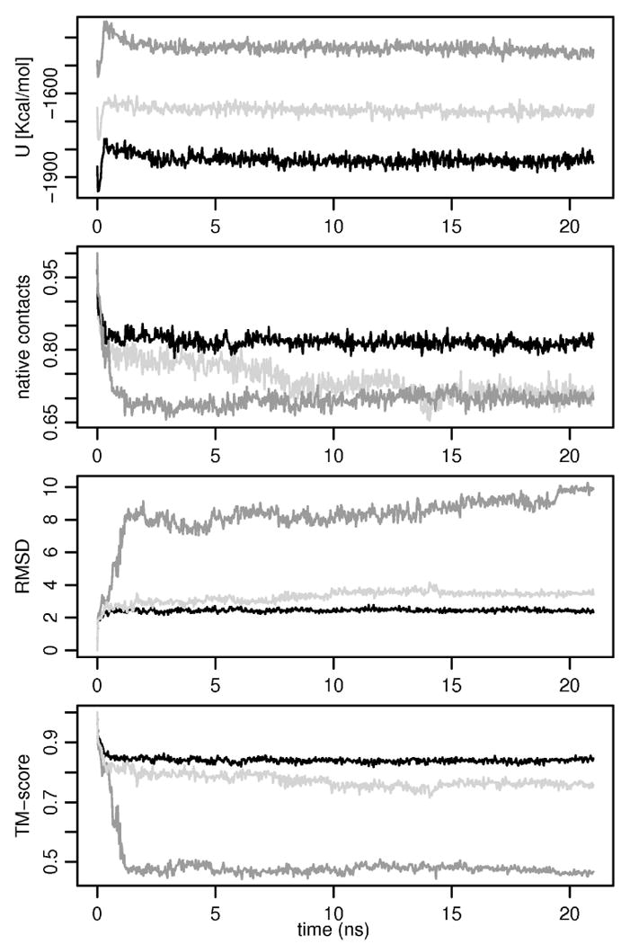
Behavior of three proteins 1a3k (an α/β protein, light gray), 1ido (an β protein, black), and 1ge6 (an α protein, dark gray) during the testing MD simulation driven by FREADY (21 ns). The figure shows from the top to the bottom the potential energy, the percentage of native contacts, the RMSD, and the TM-score.

Figure 8.

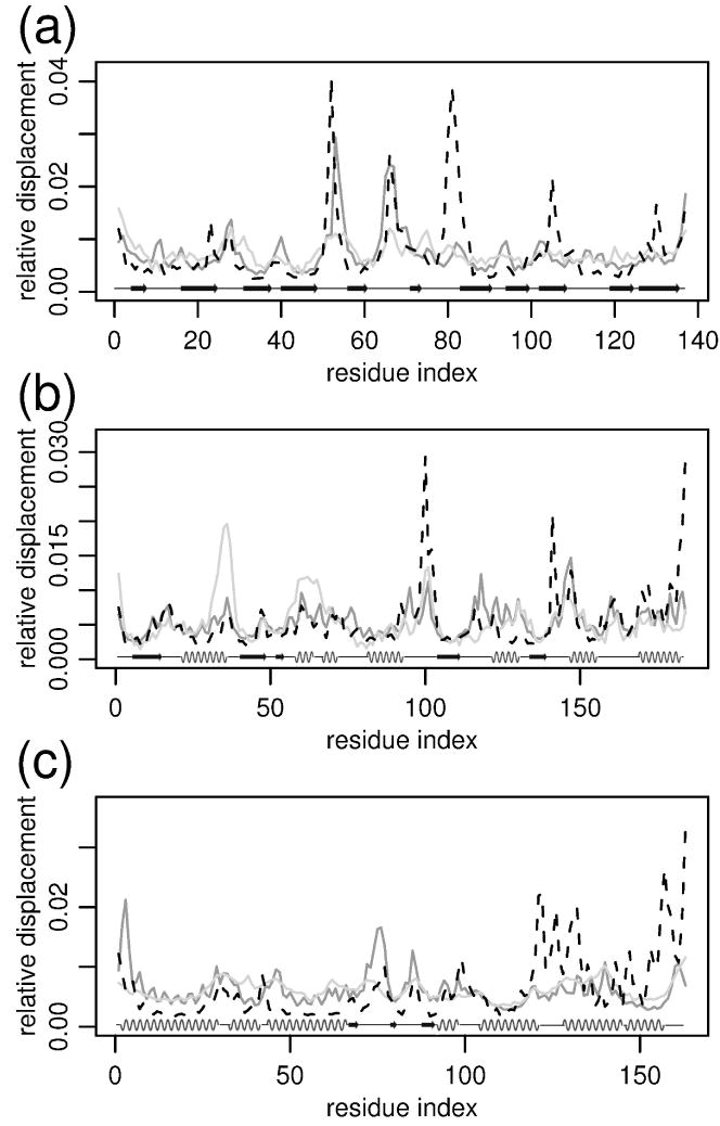
Comparison of experimental B-factors (light gray) of Cα atoms with mean square displacement in FREADY 21 ns MD simulations (black-dashed) and mean square displacements as predicted by ANM [52] from the native conformation (dark gray). The values of all methods were scaled to have equal average displacements, so only relative displacements are meaningful. The graphs correspond from top to bottom to proteins 1a3k, 1ido and 1ge6. The correlation coefficients between experimental B-factors and simulation displacements are 0.4, 0.33, and 0.3 respectively. Secondary structure elements are shown at the lower part of the figure.

Structural alignments of the final MD structures with the native conformations for these three proteins are given in Figure 9 - Figure 11. We have not found any correlation between stability of the native conformations in FREADY potential and the secondary structure content or composition (data not shown). We initially attempted to train FREADY without an explicit hydrogen bonding term. However, MD simulations of the training set driven by a potential trained without hydrogen bonding term resulted in the average deviation of 6.37 Å RMSD from the native structures compared to 4.95 Å obtained with a potential trained with explicit backbone hydrogen bonding term. The reduced accuracy in our initial attempt was caused mainly by weak stability of native β sheets elements.

Figure 9.

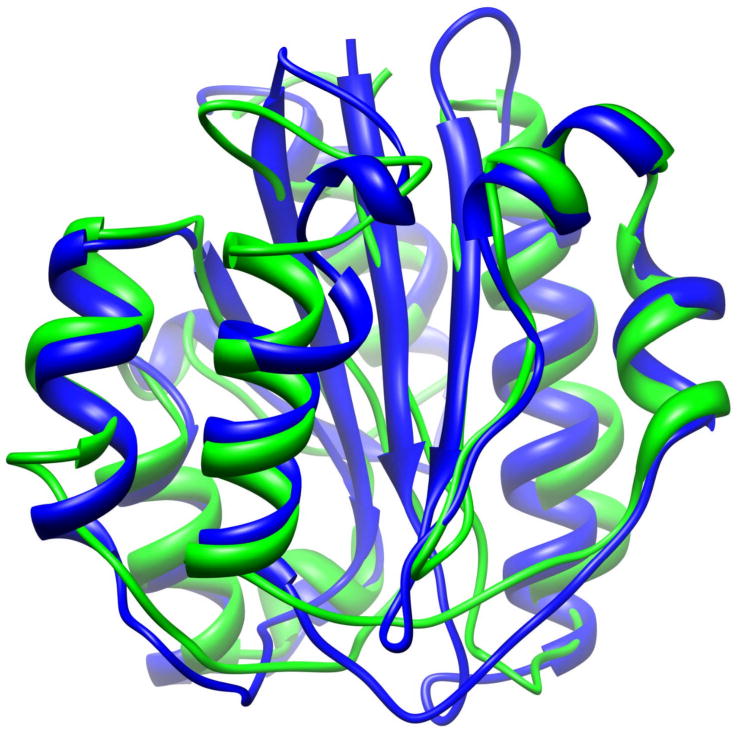
Alignment of native structure (blue) of 1ido (an α/β protein) and the conformation obtained after 21 ns of MD simulation (green). The RMSD is 2.33Å. Protein structures were aligned and visualized with UCSF Chimera tool [72].

Figure 11.

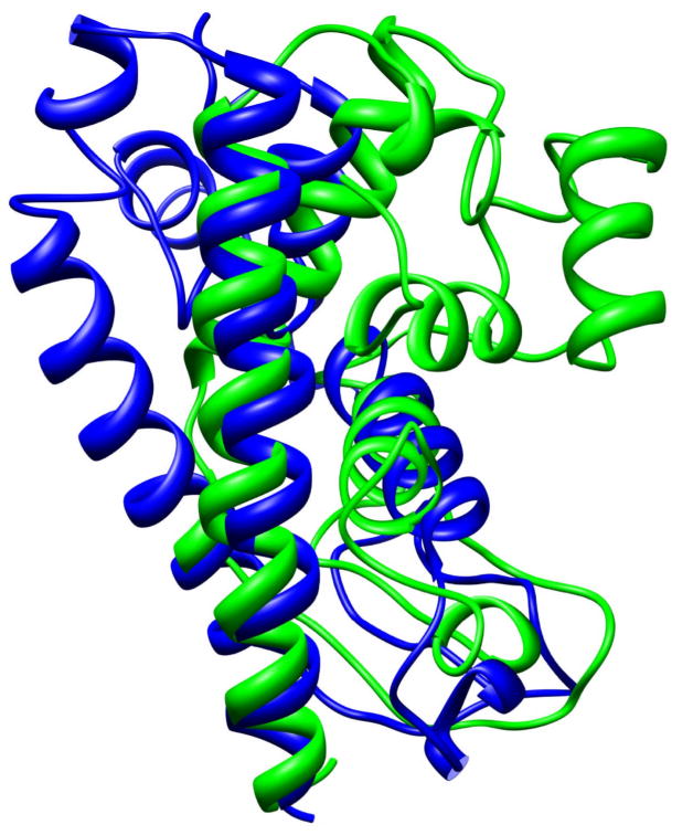
Alignment of native structure (blue) of 1ge6 (an α protein) and the conformation obtained after 21 ns of MD simulation (green). The RMSD is 9.87Å.

Better stability of native folds (3.92 Å from native in average) was reported recently by Minary and Levitt [53]. They used a 3-bead model based on an all-atomistic statistical potential [54]. There are two major differences in their approach and results presented here. More extensive conformational search with a combination of parallel tempering and equi-energy Monte Carlo was performed in their work, whereas we only ran long MD simulations. Another important difference is in the number of degrees of freedom. In the work of Minary and Levitt secondary structure elements are fixed and the loop torsional angles are considered as the only degrees of freedom. Fixing the secondary structures in the simulations that uses the FREADY potential reduces the distance (RMSD) between the simulated structures and the native conformations in the 21 ns MD simulations to 3.04 Å in RMSD. The similarity increases to 0.78 measured with the TM-score.

The FREADY potential was also tested on native and near-native recognition from a set of decoy structures. Two datasets of decoys used in this study are “Decoys ‘R’ Us” dataset [55] and the set of decoys used for the training of LOOPP [42]. Both sets consist of a collection of different models generated as possible conformations for protein sequences with known structures (targets). “Decoys ‘R’ Us” dataset includes 34 targets, each target having from 500 to 2414 different models including the native structure. In the LOOPP dataset, there are 2470 protein targets, each having from 30 to 200 models. There is no overlap between the FREADY training set and the set of targets used in the LOOPP testing dataset.

In the decoy recognition task a set of different structures with an identical sequence (i.e. the sequence of the target) is provided. The task is to score the structure closest to the native (or the native itself, if present in the input set) as the model with the lowest energy. To use FREADY for this purpose only the sum of the non-bonded interactions and the torsional energies was used. By construction, the structures of the decoys have reasonable covalent geometries. Moreover, the local interaction terms of the bond and angular stretching are quite sensitive to local modifications in the structure and do not provide significant information about the overall quality of the three-dimensional shape. Therefore bond and angle terms of FREADY are not helpful in differentiating between native and decoy shapes.

Another type of interaction with a limited contribution is the short-range repulsion. The non-bonded interaction term as learned from MD simulations has steep repulsion for short distances (see Figure 3) which is not desirable for a structure recognition task (a single close contact can significantly increase the energy of an overall good model), thus the non-bonded interaction term U_NB for short distances was reduced through a logarithmic transformation to yield an adjusted value $U_{NB}^{\prime }$

$$U_{NB}^{\prime }=0.6+\frac{log(U_{NB}+0.4)}{10}\text{if}{U}_{NB}>0.6.$$ (1.12)

The last remaining term, the backbone hydrogen bonding, was not useful in recognition, probably because decoys in the datasets were generated with methods that optimize backbone hydrogen bonds.

FREADY performs similarly (see Table 1) to other statistical potentials on “Decoys ‘R’ Us” dataset. Only OPUS-PSP potential [21], which uses more elaborate representation of side chain packing, performs significantly better than FREADY. The detailed performance of FREADY on “Decoys ‘R’ Us” dataset is provided in Table 2 and the contribution of different energy terms to the recognition in threading experiments is shown in Table 3. Seven targets from this dataset (1ctf, 1r69, 2cro, 1nkl, 1trl, 1dtk, 1shf) were present in the FREADY training set.

Table 1.

The comparison of several statistical potentials on “Decoys ‘R’ Us” dataset. Results for all potentials (except FREADY) are taken from the reference [21]. The second column lists number of targets which a given force field ranks as the lowest energy structure versus the total number of targets evaluated by that force field. The third column shows the average Z-score, $\left(\langle U\rangle -U_{\mathrm{native}}\right)/\sqrt{\langle U^2\rangle -{\langle U\rangle }^2}$, of native structures.

	Top 1/Total Number	Mean Z-sore
OPUS-PSP [21]	31/34	5.37
HPMF [56]	29/32	4.18
FREADY	28/34	4.62
DOPE [57]	28/32	-
MSE [58]	21/23	5.78
DFIRE [38]	27/32	4.52
MJ_2005 [59]	27/34	5.93
DFIRE-SCM [60]	23/32	4.36
MM-PBSA [61]	23/24	1.95
DGR [62]	21/25	5.25
DWL [63]	21/32	3.66
TE13 [64]	14/25	3.53
CALSP [65]	15/25	-
Rosetta [66]	14/32	-

Table 2.

Performance of FREADY potential on “Decoys ‘R’ Us” dataset. The table lists for each target its PDB code, size of the decoy set, rank of the native structure in the set of decoys based on FREADY energy evaluation and Z-score of the native energy.

	PDB code	Decoy set size	Rank	Z-score
4state_reduced
1	1cft	631	1	3.91
2	1r69	676	1	3.84
3	1sn3	661	1	3.83
4	2cro	675	1	3.29
5	3icb	654	1	2.57
6	4pti	688	1	4.34
7	4rxn	678	1	3.14
fisa
8	1fc2	501	336	-0.27
9	1hhd-C	501	1	3.55
10	2cro	501	1	4.55
11	4icb	501	1	5.37
fisa_casp3
12	1bg8-A	1201	1	3.91
13	1bl0	972	2	2.83
14	1eh2	2414	3	2.71
15	1jwe	1408	1	4.60
16	smd3	1201	1	6.72
lattice_ssfit
17	1beo	2001	1	7.13
18	1cft	2001	1	8.37
19	1dkt-A	2001	1	7.71
20	1fca	2001	1	6.29
21	1nkl	2001	1	7.22
22	1pgb	2001	1	9.19
23	1trl-A	2001	1	4.98
34	4icb	2001	1	8.74
lmsd
25	1b0n-B	498	16	1.62
26	1bba	501	493	-2.10
27	1cft	498	1	4.99
28	1dtk	216	1	3.12
29	1fc2	501	4	2.74
30	1igd	501	1	7.02
31	1shf-A	438	1	6.18
32	2cro	501	1	6.89
33	2ovo	348	1	3.57
34	4pti	344	1	4.48

Table 3.

Contributions of different energy terms to the recognition of native structures in Decoys R us dataset. For each energy term the number of native structures recognize as the lowest energy structure by that term is given in the first column and the average Z-score of the native structures is given in the second column. Based on this data the sum of non-bonded and torsional energy terms was used for final prediction (the last row in the table).

	Top 1(from 34)	Mean Z-score
Bonds	9	0.55
Angles	2	0.65
Torsions	14	2.45
Nonbonded term	27	4.17
Hydrogen bonding	2	1.19

On the LOOPP dataset we tested the recognition of “native like targets,” since statistical potentials tend to perform well in distinguishing the native structure from non-native ones but often fail in recognition of “close to native” conformations. Thus, in the case of LOOPP dataset, we ask how well does FREADY recognize native-like models (RMSD-wise) from other structures. FREADY ranks the model with the lowest RMSD as the lowest energy structure (within the top 5 lowest energy structures) in 50% (73%) of all 2470 targets. While clearly not perfect, FREADY provides a useful signal for model selection that when combined with other signals leads to more accurate prediction. FREADY signals were used in the LOOPP server during CASP8 exercise [67].

It turns out that FREADY performs better in recognition of structures obtained by X-ray crystallography than those obtained by NMR. The rate of best model recognition for targets solved by NMR drops to 31% (compared to 64% for structures solved by X-ray). The performance of FREADY on a subset of LOOPP dataset is shown in Figure 12. This set contains 338 targets that are single chain proteins, solved by X-ray crystallography, not forming biological complexes with other proteins or RNA/DNA, and are not membrane proteins. The correlation coefficient for this set between E/L−(E/L)_native and the RMSD from the native conformation is 0.68. As seen in the figure, only several models have lower scores than the native (negative values on the figure) and most of the native-like models (low RMSD values) do not have high scores.

Figure 12.

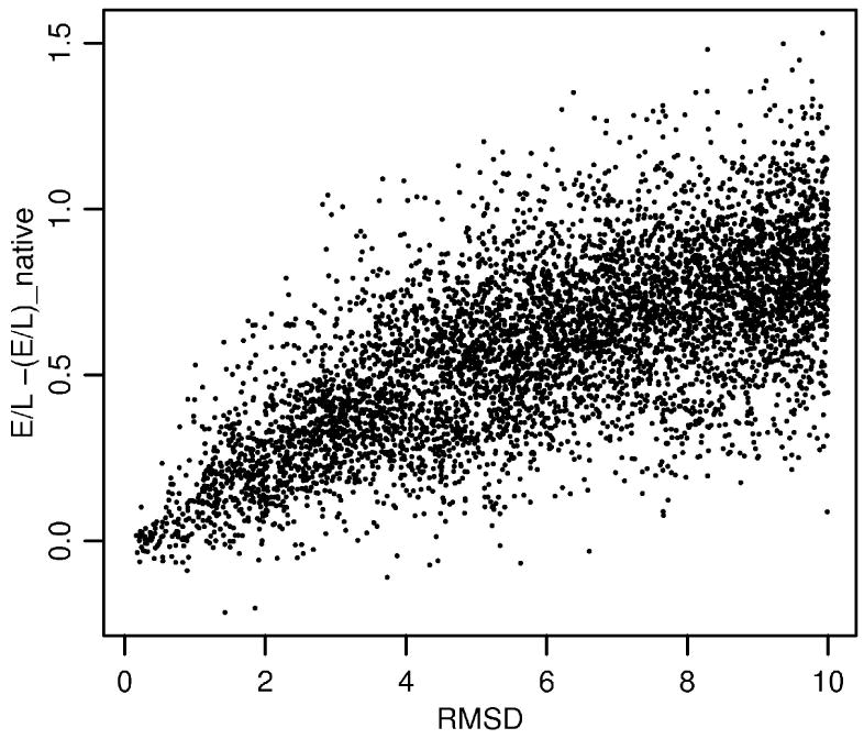
The difference of FREADY energy normalized by protein length from that of the native as a function of the RMSD from the native conformation. Each point in the figure corresponds to a model for a structure of a protein. There are 6034 models (for 338 targets) shown in the figure and only several structures score below the native conformations (negative values). On the average the energy seems a linear function of the RMS from the native suggesting a broad radius of influence for the FREADY potential.

Final remarks

In the present manuscript we discussed a coarse grained potential that was learned using a mix of machine learning arguments and computational statistical mechanics. The potential was tested and illustrated to perform adequately at the two extreme limits of structural biology: (i) maintaining the structure in the neighborhood of the native fold in Molecular Dynamics simulations, and (ii) effectiveness in threading experiments. The significantly reduced number of degrees of freedom enables more comprehensive sampling for longer times. The simpler model (compared to all atom representation) is also effective in screening efficiently a large number of candidates to the correct fold. On the other hand, we do not expect the potential to work in domains it was not tuned for (e.g. protein folding).

We have addressed algorithmically two significant limitations of statistical potentials, that is, (i) how to learn a statistical potential that recovers experimental statistics in canonical simulations and (ii) how to effectively combine statistical potentials with other energy terms that are necessary when comprehensive sampling is desired. Specifically in the present study we illustrate that the addition of hard cores and hydrogen bonding potentials is straightforward once generalized ensemble approach is applied. While hard cores could be added by statistical means [68], the iterative procedure allows for easy combination of different energy terms, potentially from different sources calibrated against the PDB distribution.

Perhaps the most intriguing observations made in the present study are the limitations of the internal coordinate representation and of the assumption of potential transferability. We typically assume that a potential can be represented by pair interactions between amino acids (keeping the covalent geometry intact). The pair interaction is assumed to be transferable from a protein to a protein. Mathematical programming studies illustrated however that the parameters of such a potential do not have a feasible solution on typical protein-like decoy sets [64, 69, 70]. It is intriguing that a related conclusion is reached in the present manuscript from a different perspective and for more general functional form.

Further studies of plausible functional forms of potentials, building on innovative work on modeling many-body potentials [24, 26, 71], with comprehensive sampling and iterative refinement of potential parameters are of considerable interest.

Figure 10.

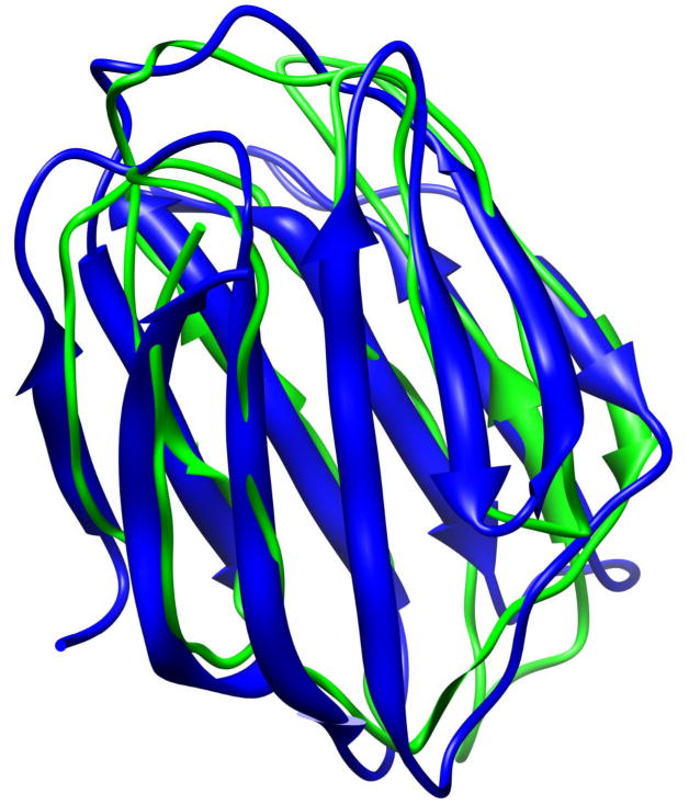
Alignment of native structure (blue) of 1a3k (a β protein) and the conformation obtained after 21 ns of MD simulation (green). The RMSD is 3.42Å.

References

- 1.Dill KA. Theory for the folding and stability of globular proteins. Biochemistry. 1985;24(6):1501–1509. doi: 10.1021/bi00327a032. [DOI] [PubMed] [Google Scholar]
- 2.Tirion MM. Large Amplitude Elastic Motions in Proteins from a Single-Parameter, Atomic Analysis. Physical Review Letters. 1996;771905(9) doi: 10.1103/PhysRevLett.77.1905. [DOI] [PubMed] [Google Scholar]
- 3.Haliloglu T, Bahar I, Erman B. Gaussian Dynamics of Folded Proteins. Physical Review Letters. 1997;79(16):3090. [Google Scholar]
- 4.Kolinski A, Skolnick J. Lattice models of protein folding, dynamics and thermodynamics. Austin, Texas: Landes Company and Chapman Hill; 1996. [Google Scholar]
- 5.Marrink SJ, et al. The MARTINI Force Field: Coarse Grained Model for Biomolecular Simulations. J Phys Chem B. 2007;111(27):7812–7824. doi: 10.1021/jp071097f. [DOI] [PubMed] [Google Scholar]
- 6.Berman HM, et al. The Protein Data Bank. Nucl Acids Res. 2000;28(1):235–242. doi: 10.1093/nar/28.1.235. [DOI] [PMC free article] [PubMed] [Google Scholar]
- 7.Miyazawa S, Jernigan RL. Estimation of effective interresidue contact energies from protein crystal structures: quasi-chemical approximation. Macromolecules. 1985;18(3):534–552. [Google Scholar]
- 8.Goldstein RA, Lutheyschulten ZA, Wolynes PG. Protein tertiary structure recognition using optimized hamiltonians with local interactions. Proceedings of the National Academy of Sciences of the United States of America. 1992;89(19):9029–9033. doi: 10.1073/pnas.89.19.9029. [DOI] [PMC free article] [PubMed] [Google Scholar]
- 9.Luthy R, Bowie JU, Eisenberg D. Assesments of protein models with 3-dimensional profiles. Nature. 1992;356(6364):83–85. doi: 10.1038/356083a0. [DOI] [PubMed] [Google Scholar]
- 10.Maiorov VN, Crippen GM. Contact potential that recognizes the correct folding of globular-proteins. Journal of Molecular Biology. 1992;227(3):876–888. doi: 10.1016/0022-2836(92)90228-c. [DOI] [PubMed] [Google Scholar]
- 11.Rizzo RC, Jorgensen WL. OPLS all-atom model for amines: Resolution of the amine hydration problem. Journal of the American Chemical Society. 1999;121(20):4827–4836. [Google Scholar]
- 12.Lagant P, et al. Increasing normal modes analysis accuracy: The SPASIBA spectroscopic force field introduced into the CHARMM program. Journal of Physical Chemistry A. 2004;108(18):4019–4029. [Google Scholar]
- 13.Wang JM, Kollman PA. Automatic parameterization of force field by systematic search and genetic algorithms. Journal of Computational Chemistry. 2001;22(12):1219–1228. [Google Scholar]
- 14.Sippl MJ. Calculation of conformational ensembles from potentials of mena force: An approach to the knowledge-based prediction of local structures in globular proteins. Journal of Molecular Biology. 1990;213(4):859–883. doi: 10.1016/s0022-2836(05)80269-4. [DOI] [PubMed] [Google Scholar]
- 15.Skolnick J, et al. Derivation and testing of pair potentials for protein folding. When is the quasichemical approximation correct? Protein Science. 1997;6(3):676–688. doi: 10.1002/pro.5560060317. [DOI] [PMC free article] [PubMed] [Google Scholar]
- 16.Betancourt MR, Thirumalai D. Pair potentials for protein folding: choice of reference states and sensitivity of predicted native states to variations in the interaction schemes. Protein Sci. 1999;8(2):361–369. doi: 10.1110/ps.8.2.361. [DOI] [PMC free article] [PubMed] [Google Scholar]
- 17.Bryant SH, Lawrence CE. An empirical energy function for threading protein-sequence through the folding motif. Proteins-Structure Function and Genetics. 1993;16(1):92–112. doi: 10.1002/prot.340160110. [DOI] [PubMed] [Google Scholar]
- 18.Hinds DA, Levitt M. Exploring conformational space with a simple lattice model for protein-structure. Journal of Molecular Biology. 1994;243(4):668–682. doi: 10.1016/0022-2836(94)90040-x. [DOI] [PubMed] [Google Scholar]
- 19.Xia Y, et al. Ab initio construction of protein tertiary structures using a hierarchical approach. Journal of Molecular Biology. 2000;300(1):171–185. doi: 10.1006/jmbi.2000.3835. [DOI] [PubMed] [Google Scholar]
- 20.Buchete NV, Straub JE, Thirumalai D. Anisotropic coarse-grained statistical potentials improve the ability to identify nativelike protein structures. The Journal of Chemical Physics. 2003;118(16):7658–7671. [Google Scholar]
- 21.Lu M, Dousis AD, Ma J. OPUS-PSP: An Orientation-dependent Statistical All-atom Potential Derived from Side-chain Packing. Journal of Molecular Biology. 2008;376(1):288–301. doi: 10.1016/j.jmb.2007.11.033. [DOI] [PMC free article] [PubMed] [Google Scholar]
- 22.Lu H, Skolnick J. A distance-dependent atomic knowledge-based potential for improved protein structure selection. Proteins-Structure Function and Genetics. 2001;44(3):223–232. doi: 10.1002/prot.1087. [DOI] [PubMed] [Google Scholar]
- 23.Hill TL. Statistical Mechanics: Principles and selected applications. New York: Dover; 1956. [Google Scholar]
- 24.Feng YP, Kloczkowski A, Jernigan RL. Four-body contact potentials derived from two protein datasets to discriminate native structures from decoys. Proteins-Structure Function and Bioinformatics. 2007;68(1):57–66. doi: 10.1002/prot.21362. [DOI] [PubMed] [Google Scholar]
- 25.Buchete NV, Straub JE, Thirumalai D. Orientational potentials extracted from protein structures improve native fold recognition. Protein Science. 2004;13(4):862–874. doi: 10.1110/ps.03488704. [DOI] [PMC free article] [PubMed] [Google Scholar]
- 26.Ngan SC, Inouye MT, Samudrala R. A knowledge-based scoring function based on residue triplets for protein structure prediction. Protein Engineering Design & Selection. 2006;19(5):187–193. doi: 10.1093/protein/gzj018. [DOI] [PMC free article] [PubMed] [Google Scholar]
- 27.Kinnear BS, Jarrold MF, Hansmann UHE. All-atom generalized-ensemble simulations of small proteins. Elsevier Science Inc; 2004. [DOI] [PubMed] [Google Scholar]
- 28.Amir EAD, Kalisman N, Keasar C. Differentiable, multi-dimensional, knowledge-based energy terms for torsion angle probabilities and propensities. Proteins-Structure Function and Bioinformatics. 2008;72(1):62–73. doi: 10.1002/prot.21896. [DOI] [PubMed] [Google Scholar]
- 29.Jagielska A, Wroblewska L, Skolnick J. Protein model refinement using an optimized physics-based all-atom force field. Proceedings of the National Academy of Sciences of the United States of America. 2008;105(24):8268–8273. doi: 10.1073/pnas.0800054105. [DOI] [PMC free article] [PubMed] [Google Scholar]
- 30.Honeycutt JD, Thirumalai D. The nature of folded states of globular proteins. Biopolymers. 1992;32(6):695–709. doi: 10.1002/bip.360320610. [DOI] [PubMed] [Google Scholar]
- 31.Brown S, Head-Gordon T. Intermediates and the folding of proteins L and G. Protein Sci. 2004;13(4):958–970. doi: 10.1110/ps.03316004. [DOI] [PMC free article] [PubMed] [Google Scholar]
- 32.Yap EH, Fawzi NL, Head-Gordon T. A coarse-grained alpha-carbon protein model with anisotropic hydrogen-bonding. Proteins: Structure, Function, and Bioinformatics. 2008;70(3):626–638. doi: 10.1002/prot.21515. [DOI] [PMC free article] [PubMed] [Google Scholar]
- 33.Aaqvist J, Warshel A. Simulation of enzyme reactions using valence bond force fields and other hybrid quantum/classical approaches. Chem Rev. 1993;93(7):2523–2544. [Google Scholar]
- 34.Maragakis P, Karplus M. Large Amplitude Conformational Change in Proteins Explored with a Plastic Network Model: Adenylate Kinase. Journal of Molecular Biology. 2005;352(4):807–822. doi: 10.1016/j.jmb.2005.07.031. [DOI] [PubMed] [Google Scholar]
- 35.Okazaki Ki, et al. Multiple-basin energy landscapes for large-amplitude conformational motions of proteins: Structure-based molecular dynamics simulations. Proceedings of the National Academy of Sciences. 2006;103(32):11844–11849. doi: 10.1073/pnas.0604375103. [DOI] [PMC free article] [PubMed] [Google Scholar]
- 36.Liwo A, et al. Parametrization of Backbone-Electrostatic and Multibody Contributions to the UNRES Force Field for Protein-Structure Prediction from Ab Initio Energy Surfaces of Model Systems. J Phys Chem B. 2004;108(27):9421–9438. [Google Scholar]
- 37.Liwo A, et al. Calculation of protein backbone geometry from {alpha}-carbon coordinates based on peptide-group dipole alignment. Protein Sci. 1993;2(10):1697–1714. doi: 10.1002/pro.5560021015. [DOI] [PMC free article] [PubMed] [Google Scholar]
- 38.Zhou H, Zhou Y. Distance-scaled, finite ideal-gas reference state improves structure-derived potentials of mean force for structure selection and stability prediction. Protein Sci. 2002;11(11):2714–2726. doi: 10.1110/ps.0217002. [DOI] [PMC free article] [PubMed] [Google Scholar]
- 39.Reith D, Pütz M, Müller-Plathe F. Deriving effective mesoscale potentials from atomistic simulations. Journal of Computational Chemistry. 2003;24(13):1624–1636. doi: 10.1002/jcc.10307. [DOI] [PubMed] [Google Scholar]
- 40.Sun Q, Ghosh J, Faller R. In: Coarse-Graining of Condensed Phase and Biomolecular Systems. Voth G, editor. Boca Raton FL: CRC press; 2008. [Google Scholar]
- 41.Hansmann UHE, Okamoto Y, Eisenmenger F. Molecular dynamics, Langevin and hydrid Monte Carlo simulations in a multicanonical ensemble. Chemical Physics Letters. 1996;259(34):321–330. [Google Scholar]
- 42.Vallat BK, Pillardy J, Elber R. A template-finding algorithm and a comprehensive benchmark for homology modeling of proteins. Proteins: Structure, Function, and Bioinformatics. 2008;72(3):910–928. doi: 10.1002/prot.21976. [DOI] [PMC free article] [PubMed] [Google Scholar]
- 43.Meyerguz L, et al. Computational analysis of sequence selection mechanisms. Structure. 2004;12(4):547–557. doi: 10.1016/j.str.2004.02.018. [DOI] [PubMed] [Google Scholar]
- 44.Tusnady GE, Dosztanyi Z, Simon I. Transmembrane proteins in the Protein Data Bank: identification and classification. Bioinformatics. 2004;20(17):2964–2972. doi: 10.1093/bioinformatics/bth340. [DOI] [PubMed] [Google Scholar]
- 45.Jayasinghe S, Hristova K, White SH. MPtopo: A database of membrane protein topology. Protein Sci. 2001;10(2):455–458. doi: 10.1110/ps.43501. [DOI] [PMC free article] [PubMed] [Google Scholar]
- 46.Spirin S, et al. NPIDB: a Database of Nucleic Acids Protein Interactions. Bioinformatics. 2007;23(23):3247–3248. doi: 10.1093/bioinformatics/btm519. [DOI] [PubMed] [Google Scholar]
- 47.Narang P, et al. A computational pathway for bracketing native-like structures for small alpha helical globular proteins. Physical Chemistry Chemical Physics. 2005;7:2364–2375. doi: 10.1039/b502226f. [DOI] [PubMed] [Google Scholar]
- 48.Jayaram B, et al. Bhageerath: an energy based web enabled computer software suite for limiting the search space of tertiary structures of small globular proteins. Nucl Acids Res. 2006;34(21):6195–6204. doi: 10.1093/nar/gkl789. [DOI] [PMC free article] [PubMed] [Google Scholar]
- 49.Elber R, et al. MOIL: A program for simulations of macromolecules. Computer Physics Communications. 1995;91(13):159–189. [Google Scholar]
- 50.Liwo A, et al. Prediction of protein conformation on the basis of a search for compact structures: Test on avian pancreatic polypeptide. Protein Sci. 1993;2(10):1715–1731. doi: 10.1002/pro.5560021016. [DOI] [PMC free article] [PubMed] [Google Scholar]
- 51.Zhang Y, Skolnick J. Scoring function for automated assessment of protein structure template quality. Proteins: Structure, Function, and Bioinformatics. 2004;57(4):702–710. doi: 10.1002/prot.20264. [DOI] [PubMed] [Google Scholar]
- 52.Eyal E, Yang LW, Bahar I. Anisotropic network model: systematic evaluation and a new web interface. Bioinformatics. 2006;22(21):2619–2627. doi: 10.1093/bioinformatics/btl448. [DOI] [PubMed] [Google Scholar]
- 53.Minary P, Levitt M. Probing Protein Fold Space with a Simplified Model. Journal of Molecular Biology. 2008;375(4):920–933. doi: 10.1016/j.jmb.2007.10.087. [DOI] [PMC free article] [PubMed] [Google Scholar]
- 54.Summa CM, Levitt M. Near-native structure refinement using in vacuo energy minimization. Proceedings of the National Academy of Sciences. 2007;104(9):3177–3182. doi: 10.1073/pnas.0611593104. [DOI] [PMC free article] [PubMed] [Google Scholar]
- 55.Samudrala R, Levitt M. Decoys ‘R’ Us: a database of incorrect conformations to improve protein structure prediction [In Process Citation] Protein Sci. 2000;9(7):1399–1401. doi: 10.1110/ps.9.7.1399. [DOI] [PMC free article] [PubMed] [Google Scholar]
- 56.Lin MS, Fawzi NL, Head-Gordon T. Hydrophobic Potential of Mean Force as a Solvation Function for Protein Structure Prediction. Structure. 2007;15(6):727–740. doi: 10.1016/j.str.2007.05.004. [DOI] [PubMed] [Google Scholar]
- 57.Shen My, Sali A. Statistical potential for assessment and prediction of protein structures. Protein Sci. 2006;15(11):2507–2524. doi: 10.1110/ps.062416606. [DOI] [PMC free article] [PubMed] [Google Scholar]
- 58.McConkey BJ, Sobolev V, Edelman M. Discrimination of native protein structures using atom-atom contact scoring. Proceedings of the National Academy of Sciences of the United States of America. 2003;100(6):3215–3220. doi: 10.1073/pnas.0535768100. [DOI] [PMC free article] [PubMed] [Google Scholar]
- 59.Miyazawa S, Jernigan RL. How effective for fold recognition is a potential of mean force that includes relative orientations between contacting residues in proteins? The Journal of Chemical Physics. 2005;122(2):024901. doi: 10.1063/1.1824012. [DOI] [PubMed] [Google Scholar]
- 60.Zhang C, et al. An accurate, residue-level, pair potential of mean force for folding and binding based on the distance-scaled, ideal-gas reference state. Protein Sci. 2004;13(2):400–411. doi: 10.1110/ps.03348304. [DOI] [PMC free article] [PubMed] [Google Scholar]
- 61.Lee M, Yang R, Duan Y. Comparison between Generalized-Born and Poisson–Boltzmann methods in physics-based scoring functions for protein structure prediction. Journal of Molecular Modeling. 2005;12(1):101–110. doi: 10.1007/s00894-005-0013-y. [DOI] [PubMed] [Google Scholar]
- 62.Dehouck Y, Gilis D, Rooman M. A New Generation of Statistical Potentials for Proteins. Biophys J. 2006;90(11):4010–4017. doi: 10.1529/biophysj.105.079434. [DOI] [PMC free article] [PubMed] [Google Scholar]
- 63.Dong Q, Wang X, Lin L. Novel knowledge-based mean force potential at the profile level. BMC Bioinformatics. 2006;7:324. doi: 10.1186/1471-2105-7-324. [DOI] [PMC free article] [PubMed] [Google Scholar]
- 64.Tobi D, Elber R. Distance-dependent, pair potential for protein folding: Results from linear optimization. Proteins: Structure, Function, and Genetics. 2000;41(1):40–46. [PubMed] [Google Scholar]
- 65.Zhang J, Chen R, Liang J. Empirical potential function for simplified protein models: Combining contact and local sequence-structure descriptors. Proteins: Structure, Function, and Bioinformatics. 2006;63(4):949–960. doi: 10.1002/prot.20809. [DOI] [PubMed] [Google Scholar]
- 66.Simons KT, et al. Improved recognition of native-like protein structures using a combination of sequence-dependent and sequence-independent features of proteins. Proteins: Structure, Function, and Genetics. 1999;34(1):82–95. doi: 10.1002/(sici)1097-0134(19990101)34:1<82::aid-prot7>3.0.co;2-a. [DOI] [PubMed] [Google Scholar]
- 67.Vallat BK, et al. Building and assessing atomic models of proteins from structural templates. doi: 10.1002/prot.22401. to be submitted. [DOI] [PMC free article] [PubMed] [Google Scholar]
- 68.Miyazawa S, Jernigan RL. Residue - Residue Potentials with a Favorable Contact Pair Term and an Unfavorable High Packing Density Term, for Simulation and Threading. Journal of Molecular Biology. 1996;256(3):623–644. doi: 10.1006/jmbi.1996.0114. [DOI] [PubMed] [Google Scholar]
- 69.Tobi D, et al. On the design and analysis of protein folding potentials. Proteins: Structure, Function, and Genetics. 2000;40(1):71–85. doi: 10.1002/(sici)1097-0134(20000701)40:1<71::aid-prot90>3.0.co;2-3. [DOI] [PubMed] [Google Scholar]
- 70.Michele V, Eytan D. Pairwise contact potentials are unsuitable for protein folding. The Journal of Chemical Physics. 1998;109(24):11101–11108. [Google Scholar]
- 71.Buchete NV, Straub JE, Thirumalai D. Development of novel statistical potentials for protein fold recognition. Current Opinion in Structural Biology. 2004;14(2):225–232. doi: 10.1016/j.sbi.2004.03.002. [DOI] [PubMed] [Google Scholar]
- 72.Pettersen EF, et al. UCSF Chimera - A visualization system for exploratory research and analysis. Journal of Computational Chemistry. 2004;25(13):1605–1612. doi: 10.1002/jcc.20084. [DOI] [PubMed] [Google Scholar]