An image-processing toolset for diffusion tensor tractography

Abstract

Diffusion tensor imaging (DTI)-based fiber tractography holds great promise in delineating neuronal fiber tracts and, hence, providing connectivity maps of the neural networks in the human brain. An array of image-processing techniques has to be developed to turn DTI tractography into a practically useful tool. To this end, we have developed a suite of image-processing tools for fiber tractography with improved reliability. This article summarizes the main technical developments we have made to date, which include anisotropic smoothing, anisotropic interpolation, Bayesian fiber tracking and automatic fiber bundling. A primary focus of these techniques is the robustness to noise and partial volume averaging, the two major hurdles to reliable fiber tractography. Performance of these techniques has been comprehensively examined with simulated and in vivo DTI data, demonstrating improvements in the robustness and reliability of DTI tractography.

1. Introduction

Diffusion tensor imaging (DTI) as a novel magnetic resonance imaging modality is rapidly becoming a primary technique for noninvasive studies of the structure of living tissue such as human brain [1]. In DTI, measurements acquired at each image voxel allow the estimation of a symmetric, second-order, positive definite matrix whose components describe the local random motion of water molecules. As the random motion of water molecules is mediated by the diffusion properties of the media in which they reside, measurements from DTI can be used to infer structural features of the tissue being imaged [2]. Since its introduction a decade ago, DTI has been used in a wide array of clinical and basic medical investigations that include cerebral ischemia [3], white matter disease [4], brain tumors [5], neuropsychic disorders [6,7] and developmental studies [8].

Originally proposed to characterize local tissue properties such as diffusion anisotropy, DTI has recently become an important utility to map neuronal fiber tracts in vivo, a technique known as diffusion tensor tractography (DTT). DTT draws upon the principle that the dominant direction of water diffusion coincides with the local tangent direction of fibrous tissue, the integration of which promises the delineation of entire fiber tracts [9]. This unique potential of DTI to map neuronal fiber tracts in vivo or, more generally, to depict the structural connectivity of the neural networks in the human brain has triggered considerable interest in the medical imaging, image analysis, computer science and medical research communities. A range of image-processing techniques such as noise reduction [10,11], interpolation [12], registration [13,14], fiber tracking [15–17], tract visualization [18,19], fiber clustering [20] and quantification [21] have to be developed to fully explore the potential. In our group, we have addressed several of the above technical issues and provided a rich set of image-processing tools for reliable fiber tractography with DTI. The intent of this article is therefore to summarize the major technical developments we have made during the past 5 years, with the hope of benefiting investigators who are interested in using DTT in their research.

The remainder of this article is organized as follows. Section 2 describes the anisotropic smoothing, an essential preprocessing procedure for DTI data. Section 3 focuses on an anisotropic interpolation technique, which has established its potential over conventional interpolation methods in fiber tracking. A novel Bayesian tracking algorithm for fiber tractography is discussed in Section 4. Finally, we present an automatic bundling algorithm for classifying neural fiber pathways in Section 5. Section 6 summarizes the main contributions of these methods, followed by some concluding remarks.

2. Anisotropic smoothing

Noninvasive characterization of living tissue is performed by analyzing the eigen parameters of the diffusion tensors in DTI data. Inhomogeneity of eigenvalues due to the anisotropic motion of water molecules is the key feature used to classify tissue architecture as well as structural integrity. The eigen parameters are susceptible to noise, which induces systematically biased assessment of structural features, such as overestimation of diffusion anisotropy and accumulation of directional errors while tracing neuronal fiber pathways [22]. Suppression of noise in diffusion tensor images is essential to improve the accuracy of the tissue’s structural and architectural characterization.

An important consideration in noise reduction is the preservation of structural boundaries. Structural boundaries define the spatial range of individual structures and offer a natural means of confining fiber-tracking process to the specific structure of interest. It is necessary to use nonlinear filtering techniques to preserve structural boundaries that are particularly rich in DTI data. To date, a number of nonlinear smoothing or regularization methods have been proposed to denoise DTI data, including nonlinear diffusion filtering [23], tensor eigen direction regularization based on a Markovian model [10], stochastic relaxation labeling [24], variational principles [25,26] and constraint preserving flow [27]. However, these sophisticated methods were not rigorously validated with in vivo human DTI data to establish their practical utility, and therefore, the DTI community still resorts to more basic methods such as Gaussian smoothing [28]. The anisotropic smoothing technique discussed here is developed with a similar concept of anisotropic diffusion filtering, originally proposed by Weickert [29] to enhance flow-like structures in scalar images. We will describe briefly in the following our novel formulation of an elegant smoothing kernel that can restore the tensor directional information while preserving the structural boundaries in DTI data. Experiments with simulated and in vivo DTI data demonstrate that this operationally simple method can effectively reduce the impact of noise on the tensor principal eigen direction [30], which offers the potential of using it as a routine utility.

2.1. Smoothing kernel construction

As with conventional implementations, our anisotropic image smoothing employs a partial differential equation:

$$\frac{\partial \mathbf{I}}{\partial t}=\text{div}(\mathbf{T}·\nabla \mathbf{I}),$$ (1)

where I is the image intensity, ∇I is the intensity gradient and t is the iteration “time” parameter. T is a structure tensor that determines the behavior of smoothing. For anisotropic smoothing, T can be constructed from the intensity gradient tensor G, which is obtained by convolving the outer product of ∇I with a Gaussian kernel K_ρ (ρ is the standard deviation of the Gaussian kernel):

$$\mathbf{G}={{\mathbf{K}}_{\rho }}^{*}(\nabla \mathbf{I}\otimes \nabla \mathbf{I})\text{.}$$ (2)

The eigen system of the gradient tensor G characterizes the local image structure, with the major eigenvector (corresponding to the largest eigenvalue) perpendicular to the local contrast boundary and the minor eigenvector (corresponding to the smallest eigenvalue) parallel to it. In our design, T is defined as a normalized inverse of G [30]. As a result, at structural boundaries, the eigenvalue of the structure tensor is small across the structural boundary but large along it. This allows anisotropic smoothing, that is, greater smoothing along the tangential direction of contrast boundaries than perpendicular to it. However, in homogeneous regions, the three eigenvalues of T have similar magnitude, resulting in an isotropic smoothing as desired.

Our anisotropic smoothing is performed on diffusion-weighted images (DWIs) from which diffusion tensors are derived. As there are multiple weighting directions, we use a common gradient tensor for all weighting directions in order to capture the boundary information that is not present in all directions. This can be simply done by summing ∇I⊗∇I over all directions, followed by a component-wise convolution with a Gaussian kernel K_ρ.

2.2 Smoothing experiments

2.2.1. Simulated DTI data

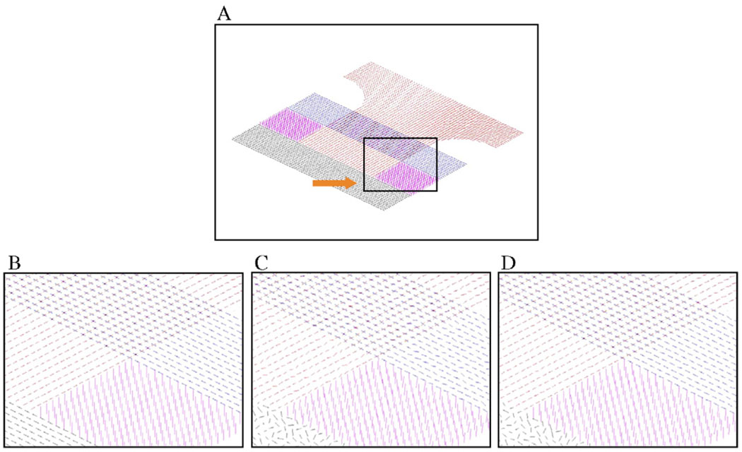
The anisotropic smoothing algorithm was tested with simulated DTI data synthesized with in vivo diffusion parameters of the human brain. Fig. 1A shows two slices of synthetic “fibers” with different colors denoting different orientations. The fibers were axially symmetric with a mean diffusivity (D) of 0.7 × 10⁻⁵ cm²/s and a fractional anisotropy (FA) of 0.9. There was a region of isotropic diffusion, denoted as black in Fig. 1, that had D = 0.7 × 10⁻⁵ cm²/s and FA = 0. The DWIs from which diffusion tensors are calculated were noise free, but zero mean Gaussian noise was added with a standard deviation equal to 0.10 times the image intensity, generating noisy simulated data. The noisy data were subsequently subjected to 50 iterations of anisotropic smoothing.

Fig. 1.

Effect of anisotropic smoothing on simulated data. (A) Middle portion of the noiseless simulated data. The line segments represent the PDD, and different colors denote different orientations of “fiber” bundles. (B) Enlarged view of the black boxed region in Panel A. (C) PDDs after adding zero mean Gaussian noise to simulated data (S.D. = 0.10). (D) PDDs after 60 iterations of anisotropic smoothing.

2.2.2. In vivo human data

A set of DWIs was acquired from a healthy human subject with the use of a 3-T GE Signa magnetic resonance scanner (General Electric, Milwaukee, WI) to study the performance of the algorithm on in vivo DTI data. A volume of 250 × 250 × 120 mm³ was scanned using six noncollinear weighting directions and a single-shot, echo-planar, pulsed gradient spin-echo imaging sequence with a b value of 1000 s/mm². The data matrix acquired had a size of 128 × 128 × 34 and was latter interpolated to be 256 × 256 × 34. Eight repeated scans were obtained and averaged to yield a volume data set with high signal-to-noise ratio (SNR ~70). This data set was corrupted with zero mean Gaussian noise at a standard deviation equal to 0.10 times the DWI intensity and smoothed for 50 iterations of anisotropic smoothing.

2.2.3. In vivo monkey data

Performance of the algorithm was also tested on a set of ex vivo monkey (owl) brain images acquired on a 9.4-T magnet using a T₂-weighted multishot spin-echo pulse sequence (TE = 31.15 ms, TR = 17.1 ms). The image array dimension was 128 × 128 × 132 voxels, and the spatial resolution was 0.3 × 0.3 × 0.3 mm³. The original data had a low SNR of 5.5, and hence, the algorithm was tested directly on the data without adding noise to it.

2.3. Experimental results

2.3.1. Simulated data

The effect of anisotropic smoothing on simulated DTI data is demonstrated in Fig. 1B–D. Fig. 1B is an enlarged view of the boxed region in Fig. 1A. Fig. 1 shows the effect of adding zero mean Gaussian noise (S.D. = 0.10) to the simulated data (Panel C) and the result after 60 iterations of anisotropic smoothing (Panel D). The variations in the principal diffusion direction (PDD) due to noise are significantly reduced after smoothing, and no blurring of the PDD near boundaries is observed. The PDDs in the isotropic region (marked by an arrow in Fig. 1A) are not consistently reoriented after smoothing, which is quite obvious since this region has no fibers and, presumably, has no directional preference.

2.3.2. In vivo human data

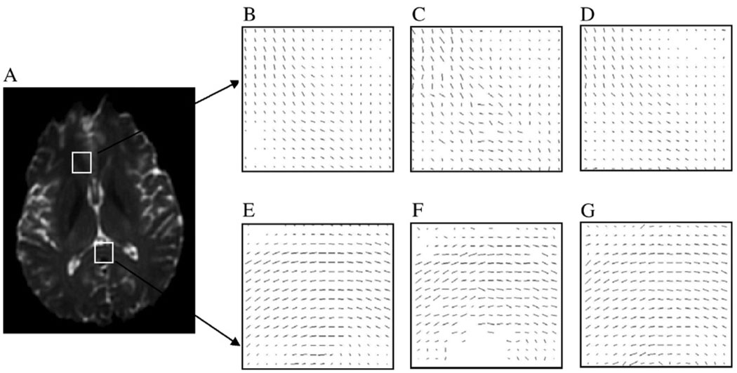
The effect of anisotropic smoothing on two representative regions in the human brain is demonstrated in Fig. 2. The upper row (Panels B, C and D) contains white matter in the frontal area where fiber tracts with distinct orientations exist. The lower row (Panels E, F and G) contains a portion of the corpus callosum with largely parallel neuronal fibers. Fig. 2B and E shows the in-plane component of the PDD (weighted with FA) of the “gold standard” data; Fig. 2C and F shows the effect of adding zero mean Gaussian noise (S.D. = 0.10) to Fig. 2B and E; Fig. 2D and G shows the results after applying 60 iterations of anisotropic smoothing to Fig. 2C and F. It can be seen that the anisotropic smoothing significantly reduces the impact of noise on the PDD in both regions.

Fig. 2.

Demonstration of the effect of anisotropic smoothing on two selected regions in the human DTI data. (A) A T₂-weighted image of a slice of the human brain. (B and E) In-plane component of PDDs in the boxed regions in Panel A. (C and F) PDDs after adding zero mean Gaussian noise (S.D. = 0.10) to the image data for the region in Panels B and E. (D and G) PDDs after 60 iterations of anisotropic smoothing.

2.3.3. In vivo monkey data

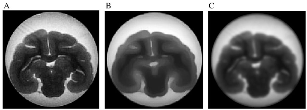
Fig. 3 shows a T₂-weighted anatomic image of the monkey brain (Panel A), the image after 25 iterations of anisotropic filtering (Panel B) and the image after 3 iterations of Gaussian (isotropic) filtering (Panel C). The result in Panel B seems to be more favorable as the boundaries are well preserved but the homogenous regions are smoothed. Compared with anisotropic smoothing, Gaussian smoothing is insensitive to image gradient; hence, structural boundaries are blurred.

Fig. 3.

Anatomic map of a T₂-weighted monkey brain image (A). Effect of anisotropic smoothing after 25 iterations (B) and Gaussian smoothing after 3 iterations (C).

3. Anisotropic interpolation

Fiber tracking with DTI is typically a reconstruction procedure to trace continuous curves from a direction field. The discrete nature of DTI data necessitates interpolation. In conjunction with smoothing, interpolation of the direction field allows fiber pathways to be tracked more reliably and in a continuous manner. Similar to smoothing, preservation of structural boundaries is also desirable in DTI data interpolation.

Interpolation is a classical image-processing problem for which a plethora of methods exists [31]. However, only a few conventional interpolation techniques have been chosen for DTI data, such as linear [32], low-order polynomial [33,34], cubic B-spline [11] and nearest-neighbor interpolations [35]. These interpolation methods differ from each other in their frequency response, extent of support, computational complexity and degree of continuity. A common feature of these methods is the use of an isotropic, space-invariant interpolation kernel that has the drawback of disregarding local image features (structural boundaries). In fact, except for the nearest-neighbor interpolation, which necessarily incurs discontinuity artifacts, all the other methods used suffer from boundary blurring.

Motivated by the need for a smooth, continuous and boundary-preserving interpolation method so that fiber pathways can be reconstructed reliably and confined within the boundary of targeted structures, we have developed a space-variant, anisotropic interpolation technique that ensures the continuity of the direction field and that, meanwhile, preserves structural boundaries [36]. Similar to the anisotropic smoothing in the preceding section, the anisotropic interpolation kernel we designed is adaptable to the local image intensity gradient profile, which is a function of the strength and orientation of contrast boundaries.

3.1. Space-variant and anisotropic data interpolation

The core part of our interpolation technique is a sigmoid function whose shape can be regulated by control parameters. Eq. (3) is the sigmoid kernel function that governs the interpolation process for the 1-D case with a range of x = [0, 1):

$$f(x)={(1+\text{exp}(a\times (x-\eta )))}^{-1}.$$ (3)

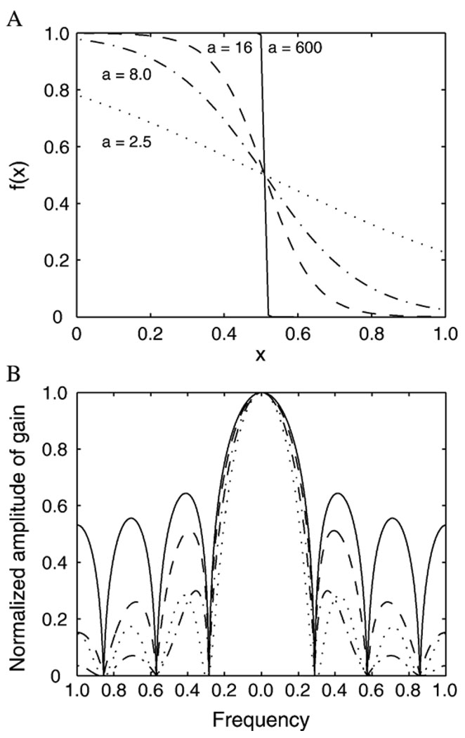
The profile of the function f(x) depends on the values of a and η, with a regulating the sharpness of the function and η controlling the position of maximum transition. Fig. 4A shows the profiles of f(x) for η = 0.5 with different values of a; their corresponding frequency responses are shown in Fig. 4B. It can be observed that large values of a produce a sharp transition in f(x), showing large gain for high-frequency components. In particular, when a approaches infinity, f(x) becomes a step function, which corresponds to nearest-neighbor interpolation. Conversely, when a = 0, f becomes a constant (equal to 0.5), which corresponds to linear interpolation (smoothing) with averaged neighborhood information. Between the two extremes, the kernel function may have various degrees of sharpness depending on the magnitude of a.

Fig. 4.

(A) Profiles of 1-D sigmoid function with different values of shape control parameter a and (B) their corresponding frequency responses. Line styles denote different values of a (and are the same in both panels).

For space-variant, anisotropic interpolation of 2-D or 3-D scalar images, we may adapt the sharpness of the sigmoid function to the local image intensity gradient. A simple form is to relate parameter a linearly to the magnitude of the intensity gradient along each spatial direction:

$$a_i=a_{\text{max}}\times \left|\frac{\nabla I_i}{\nabla I_{\text{max}}}\right|,i\in \{1,2\}\text{or}i\in \{1,2,3\},$$ (4)

where a_max sets the maximum allowable sharpness of the sigmoid function and ∇I_max is the maximum intensity gradient of the image. For interpolation of DTI data, we simply apply the anisotropic interpolation as described above to each of the six independent tensor components with a single interpolation kernel, using the mean intensity gradient of the six tensor components. This yields better data consistency, such as tensor orientational coherence and positive definiteness, than using a separate interpolation kernel for each tensor component.

3.2. Evaluation of interpolation with fiber tracking

To assess the performance of the anisotropic interpolation and to compare this with conventional methods, we performed fiber tracking with simulated and in vivo human DTI data. Fiber tracking was implemented using a streamline approach [15]. Although more sophisticated fiber-tracking methods are available (see next section), we deliberately chose this simple, intuitive approach because it simplifies the interpretation of the impacts of various interpolation techniques. For both simulated and in vivo data, the step size used was 0.2 voxel and the termination criteria were FA < 0.15 and turning angle θ > 45°. Four different values of a_max (5, 10, 15 and 20) were used for the anisotropic interpolation. Tracking results were compared with four conventional interpolation methods that include linear, nearest-neighbor, cubic polynomial and spline interpolations.

3.2.1. Simulated data

The simulated data consisted of parallel 3-D spirals that had a rectangular cross section of 3 × 9 voxels and spanned two full cycles (from 0 to 4π). Tensors for the synthetic fibers had a mean diffusivity of 0.7 × 10⁻⁵ cm²/s and an axial symmetry with an FA of 0.9, and they were aligned with the tangential direction of the tract. The synthetic fibers were embedded in an isotropic media (FA = 0), generating a volume of 128 × 128 × 30 voxels with a spatial resolution of 2 × 2 × 2 mm³.

3.2.2. In vivo data

The in vivo DTI data were acquired similarly as in Section 2.2. Streamline fiber tracking with different interpolation methods was launched from seed points defined in the corpus callosum and terminated when any of the termination criteria was satisfied.

3.3. Experimental results

3.3.1. Simulated data

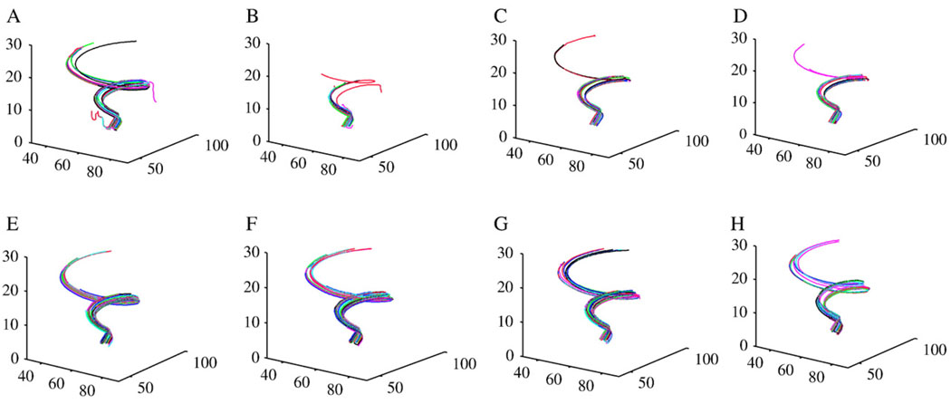
Fig. 5 shows the fibers tracked from the synthetic 3-D spirals using conventional interpolation methods (Panels A–D) and the anisotropic interpolation approach with different values of a_max (Panels E–H). Compared with the conventional interpolations, anisotropic interpolation produces more favorable results because, in general, it yields larger numbers of fibers and their pathways are more consistent.

Fig. 5.

“Fiber” tracts reconstructed from the synthetic spirals. Panels A–D are from linear, nearest-neighbor, cubic polynomial and spline interpolations, respectively. Panels E–H are from the anisotropic interpolation with a_max = 5, 10, 15 and 20, respectively.

3.3.2. In vivo data

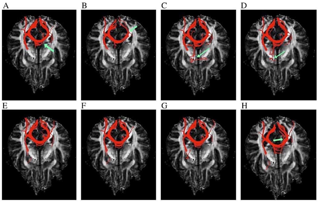
Fig. 6 shows the axial view of the anatomic structure of a fiber bundle in the corpus callosum using conventional interpolation methods (Panels A–D) and the anisotropic interpolation approach (Panels E–H). Linear interpolation (Panel A) yields fibers similar to anisotropic interpolation with a_max = 5 but generates fewer fibers than anisotropic interpolation with a_max = 10–20 (as pointed by a green arrow in Panel A). Nearest-neighbor interpolation (Panel B) yields fewer fibers than the other methods due to its inherent noise sensitivity (e.g., see the green arrow in Panel B). Fibers tracked with cubic polynomial (Panel C) and spline (Panel D) interpolations have possible wrong connections (as pointed by green arrows). These questionable connections, however, are not present in the fibers tracked with the anisotropic interpolation. In our approach, although major patterns of the fiber tracts are grossly similar, different values of a_max produce appreciable differences to the fiber structure, with the results for a_max = 10 (Panel F) and 15 (Panel G) being more plausible.

Fig. 6.

Axial view of reconstructed fibers seeded in the corpus callosum. Panels A–D are from linear, nearest-neighbor, cubic polynomial and spline interpolations, respectively, and Panels E–H are from the anisotropic interpolation with a_max = 5, 10, 15 and 20, respectively. Arrows in Panels A and B point to missed fibers, and arrows in Panels C, D and H point to possibly wrong connections.

4. Fiber tractography with Bayesian tensor regularization

In the previous section, fiber tractography was implemented using the most intuitive and basic procedure — the “streamline” approach. The purpose is to avoid other confounding factors that may complicate the comparisons of different interpolation techniques. With the streamline method, fibers are tracked by successively following the major eigenvector of the diffusion tensor. The tensor major eigenvector, however, may be an incorrect estimate of the true direction of the underlying fascicle due to the effect of image noise or partial volume averaging (PVA), which renders an unreliable basis for fiber path propagation. Although there are a number of sophisticated fiber-tracking algorithms that can mitigate the effect of noise and/or PVA [24,34,37–41], to date, fiber tractography still relies on more basic methods such as the Euler method [15] and the FACT method [35] due to their better trade-off between reliability and computational complexity over the sophisticated methods.

Motivated by the need for fiber-tracking algorithms that are not only robust to noise and PVA but also practically useful, we have developed a novel tracking algorithm based on Bayesian tensor regularization. With this framework, the uncertainty of the diffusion tensor due to noise and PVA and the variance among the tensors are incorporated into models of the conditional and a priori probabilities on the basis of multivariate normal distributions; the true local tangent direction of the underlying fascicle is estimated from an optimal solution to the Bayes decision problem with maximum a posteriori probability. Simulated and in vivo fiber-tracking experiments have demonstrated that this novel fiber-tracking algorithm allows fiber tracts to be more faithfully reconstructed than the basic streamline method.

4.1. Bayes decision rule for fiber tracking

Bayes decision is the process of determining the value of μ that maximizes the a posteriori probability P(μ_j|d); that is,

$$\mu =\underset{{\mu }_{i=1‥n}}{\text{arg max}}(P({\mu }_{j}d))=\underset{{\mu }_j}{\text{arg max}}(p(d{\mu }_j)P({\mu }_j)),$$ (5)

where P(μ_j) is the a priori probability of state μ_j and p(d|μ_j) is the conditional probability density of an observed variable d [equal to (D₁₁D₂₂D₃₃D₁₂D₁₃D₂₃)^t] if the state is μ_j. When applied to fiber tracking, the Bayes decision allows us to infer from an observed tensor the true fiber direction with maximum a posteriori probability. The a priori and conditional probability functions need to be defined to determine the true direction.

Let us assume d to be multivariate normal: d~N(μ, ∑), where μ represents the unknown true tensor and Σ is the covariance matrix. The conditional probability density of d given μ_j is

$$p(d|{\mu }_j)=\frac{1}{2\pi |\sum {|}^{1/2}}\text{exp}\left[-\frac{1}{2}{(d-{\mu }_j)}^t{\sum }^{-1}(d-{\mu }_j)\right].$$ (6)

The a priori probability P(μ_j) is also assumed to be multivariate normal: μ_j~N(m, S), where m is the mean tensor and S is the covariance matrix.

$$P({\mu }_j)=\frac{1}{{(2\pi )}^3|S{|}^{1/2}}\text{exp}\left[-\frac{1}{2}{({\mu }_j-m)}^t{S}^{-1}({\mu }_j-m)\right]$$ (7)

With Eq. (6) and Eq. (7), the solution to Eq. (5) can be found analytically according to

$$\mu ={({\sum }^{-1}+S^{-1})}^{-1}({\sum }^{-1}d+S^{-1}m).$$ (8)

Thus, the major eigenvector of μ represents the local tangent direction of fascicles with maximum a posteriori probability. Fiber tracking with this eigenvector as the propagation vector should track the fiber path with a minimum rate of error and decreased uncertainty (see Ref. [42] for essential parameter estimations).

4.2. Fiber-tracking experiments

4.2.1. Simulated data

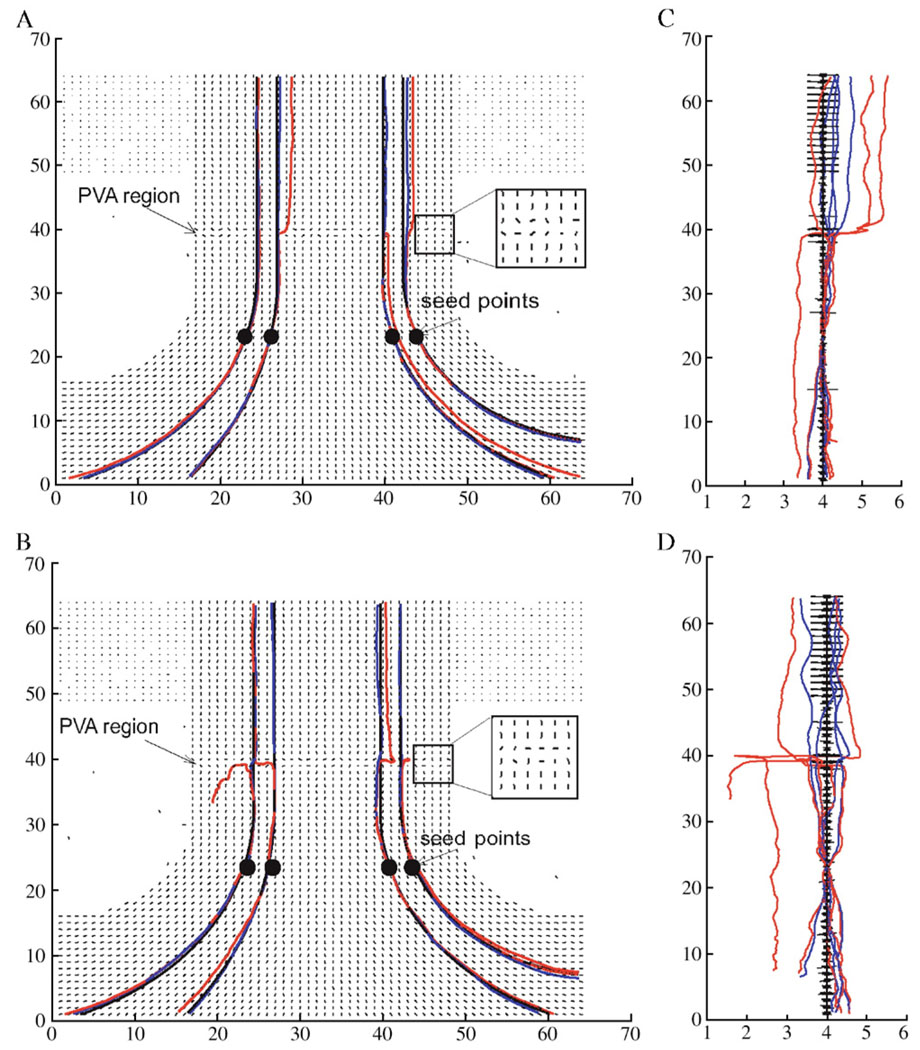
A synthetic data set was designed to contain six identical layers of straight and low planar curvature fibers. A PVA region with a width of two voxels was created around the middle portion of the straight fibers (see Fig. 7). Simulated tensors for the PVA region were spherically symmetric (λ₁ = λ₂ = λ₃); otherwise, tensors were cylindrically symmetric (λ₁ > λ₂ = λ₃) with an eigenvalue contrast (λ₁–λ₃) of 0.8 × 10⁻⁵ cm²/s. Zero mean Gaussian noise (SNR = 30 in Panels A and C and SNR = 20 in Panels B and D) was added to the data set. Fiber tracking on these noisy data sets was initiated from four seed points as shown in the figure. Four “true tracts” were obtained by tracking from the seed points with the Euler method on the noise and PVA free data set, and the performance of the Euler and Bayesian methods was compared after adding noise.

Fig. 7.

Front (A and B) and side (C and D) views of fibers tracked from synthetic data at SNR of 30 (A and C) and 20 (B and D) with a PVA region around the middle portion of the straight fibers. Red and blue curves are fibers from the Euler and Bayesian methods, respectively, and black curves are the “true fibers”. Four seed points are denoted with black dots in Panels A and B. The black line segments denote the direction of the major eigenvector at each voxel. Note the expanded scale of the abscissa in Panels C and D.

4.2.2. In vivo data

The same set of in vivo data used in the previous section was utilized to demonstrate the advantage of the Bayesian tracking algorithm in conjunction with anisotropic interpolation. A noisy DWI data set was generated by adding zero mean Gaussian noise to the original DWI data (to simulate an SNR = 20). Fibers were then tracked from the high SNR and the noisy data set with the Bayesian algorithm and anisotropic interpolation. The study focused on one major fiber bundle: the superior longitudinal fasciculus. This tract was chosen because of its well-known anatomy, thus making it possible to judge the quality of reconstructed fibers and identify erroneous connections. Fiber tracking of the same bundle was also conducted using the Euler method with linear interpolation for performance comparison.

4.3. Experimental results

4.3.1. Simulated data

Fig. 7 shows front (Panels A and B) and side (Panels C and D) views of “fiber tracts” traced from the synthetic data with the Euler (red lines) and Bayesian (blue lines) methods. The top (Panels A and C) and bottom (Panels B and D) rows have an SNR of 30 and 20, respectively. In these figures, all the fibers successfully penetrate the PVA regions with the Bayesian method but not with the Euler method; by referring to the true tracts (black lines), it can be seen that fibers tracked with the Bayesian method are more faithful than those of the Euler method.

4.3.2. In vivo data

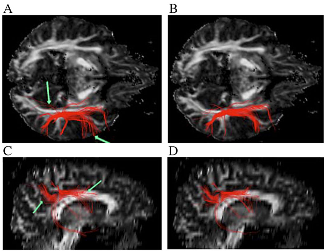
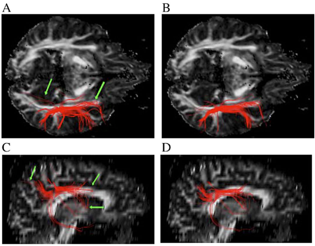
Fig. 8 shows the axial (top row) and sagittal (bottom row) views of fiber tracts seeded in the superior longitudinal fasciculus tracked with the Euler method (Panels A and C) and the Bayesian method with anisotropic interpolation (Panels B and D). The former method uses the linear interpolation technique so that appreciable changes associated with the Bayesian tracking and anisotropic interpolation can be well judged. The interpolation control parameter a_max in this case is fixed at 10 since this value produced good results in our previous experiment [36]. The Euler method produces a few erroneous connections (as pointed by green arrows in Panels A and C) that are absent with the Bayesian method. This may be explained by the sensitivity of the Euler method to noise and PVA; it can be appreciated with close inspection that, due to its noise immunity, the tracts from the Bayesian approach with anisotropic interpolation appears smoother. Fig. 9 shows both views of the fiber tracts from the same seed points but with zero mean Gaussian noise (SNR = 20) added to the data. Fibers from the Bayesian method also appear to be more favorable in this case. Compared with Fig. 8, noise seems to induce minor changes to fiber tracts from the Bayesian method but adds a few erroneous connections (as pointed by green arrows) to the fiber tracts from the Euler method.

Fig. 8.

Axial (A and B) and sagittal (C and D) views of reconstructed fiber tracts seeded in the superior longitudinal fasciculus from the original high-quality data. The left column (A and C) shows the fibers using the Euler method (linear interpolation), and the right column (B and D) shows fibers using the Bayesian method (anisotropic interpolation). Green arrows point to erroneous pathways using the Euler method.

Fig. 9.

Axial (A and B) and sagittal (C and D) views of reconstructed fiber tracts seeded in the superior longitudinal fasciculus from noisy data (SNR = 20). The left column (A and C) shows the fibers using the Euler method (linear interpolation), and the right column (B and D) shows fibers using the Bayesian method (anisotropic interpolation). Green arrows point to additional erroneous pathway using the Euler method.

5. Classification of fiber pathways

Most of the work in the literature focuses on the development of algorithms to reconstruct neuronal fiber pathways. However, there has been little research on postprocessing of reconstructed fibers, such as classifying fibers as members of distinct anatomical structures. Fiber pathways connecting the same functional regions of the brain tend to form a natural anatomical group (bundle), and those belonging to the same bundle usually are clustered in 3-D space, are approximately parallel to each other and constitute a distinct structure from other fiber bundles. In this section, we focus on the development of computer algorithms to bundle reconstructed fiber pathways into natural groups, which may provide a better means of quantifying their physical and geometric properties.

5.1. Fiber bundling with K most-similar-fibers algorithm

Fiber bundling is a typical clustering problem. In cluster analysis, partitioning of a data set into natural clusters may be achieved hierarchically or nonhierarchically. Hierarchical methods include divisive and agglomerative approaches [43]. Divisive approaches involve splitting the whole data set successively until a stop criterion is reached, while agglomerative approaches operate in the opposite direction. For clustering of fiber pathways, we employ a “K most-similar-fibers algorithm” to partition a set of fibers automatically into different natural bundles. This algorithm is conceptually similar to the “K nearest-neighbors algorithm” [44], which belongs to agglomerative methods.

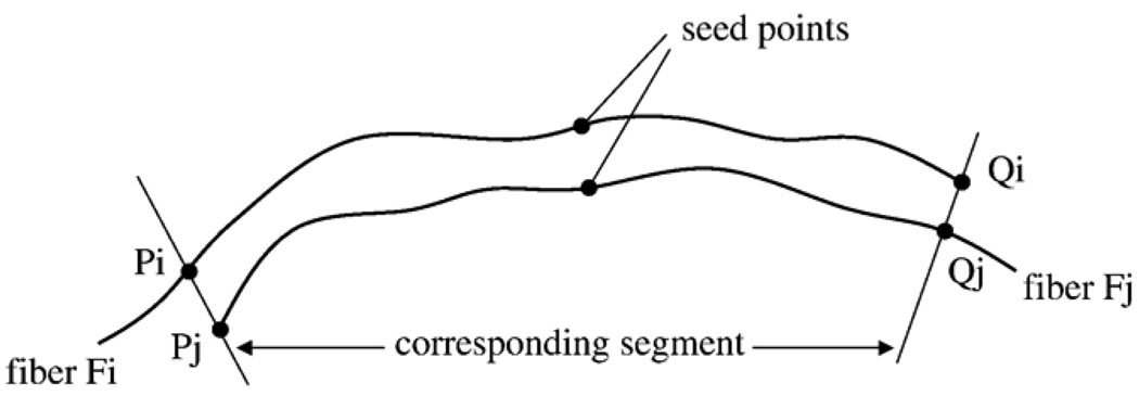
The process of fiber bundling begins with a definition of a similarity measure between a pair of fibers. First, we introduce the concept of a corresponding segment, which is loosely defined as the portion of a fiber (F_i) that has point-wise correspondence to a portion of another fiber (F_j), as illustrated in Fig. 10. Segment P_iQ_i of fiber F_i is the corresponding segment to the segment P_jQ_j of fiber F_j and vice versa. A corresponding segment ratio is then defined as the ratio of the length of the corresponding segment to the overall length of the pair of fibers:

$$R_{\text{cs}}=\frac{L_{\text{cs}}}{L_i+L_j-L_{\text{cs}}},$$ (9)

where L_cs is the length of the corresponding segment and L_i and L_j are the length of F_i and F_j, respectively. The corresponding segment ratio varies between 0 (no overlap) and 1 (each fiber completely overlaps the other). Two fibers are considered similar only when they have comparable length and similar shape and when they are separated by a small distance. The shape similarity and closeness are indicated by the mean Euclidean distance D. Therefore, the similarity between a pair of fibers can be defined by

$$S_{ij}=R_{\text{cs}}\times \text{exp}(-D/C),$$ (10)

where C is a scaling coefficient. With the definitions of corresponding segment ratio and similarity, the bundling algorithm proceeds with the following steps:

1. For a fiber F, find eight fibers whose seed points are the neighbors of the seed point of F.

2. Calculate similarity S between F and each of the eight neighboring fibers.

3. Threshold similarity such that any similarity value smaller than T (0 ≤ T ≤ 1) is set to 0.

4. Find up to K neighboring fibers whose nonzero similarity to F are greatest.

5. Group F with each of the fibers found in Step 4.

Fig. 10.

Definition of the corresponding segment. P_iQ_i of F_i is the corresponding segment to P_jQ_j of F_j. See text for explanations.

The above steps are repeated until all fibers are processed. The parameters T and K determine the characteristics of resulting fiber bundles. The threshold T with an appropriate value precludes bridging of neighboring bundles, while the number of most-similar-fibers K decides the compactness of each fiber bundle [21].

5.2. Experimental results

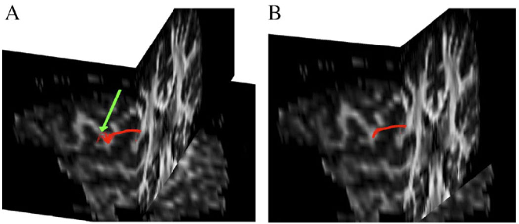
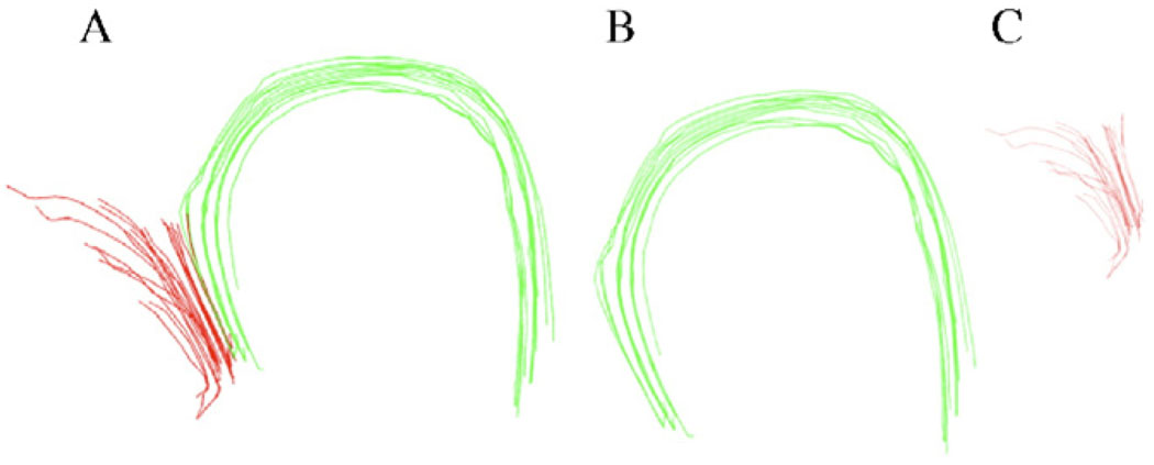
Once again, we used the same in vivo data as in the previous section to bundle the fibers. The fiber pathways were extracted from a representative location (using the Euler method) that connects superior to posterior corona radiata in the cortex. The sagittal and coronal images (Fig. 11A and B) are displayed simultaneously to provide a better understanding of connection between the two locations. The green arrow in Panel A shows a possible erroneous connection that belongs to a different bundle. Applying the bundling algorithm, the fibers were separated into two distinct bundles. Fig. 12A shows the set of fiber pathways in greater detail. The fibers could be clustered into bundles with a typical value of T = 0.16 in this case. However, in case of more complex fiber structures, a certain value of T may result in more than two bundles where bundles containing fewer and/or erroneous fibers may be excluded based on the knowledge of known anatomy. Optimization of the threshold parameter T is an empirical issue and needs better understanding of known fiber anatomy to decide its magnitude on a trial basis.

Fig. 11.

A bundle of fibers connecting superior to posterior corona radiata (A) using the Euler method. The green arrow shows an erroneous connection to the left side of the bundle, which could be effectively bundled into two groups. The major fiber bundle connecting the two regions is shown in Panel B.

Fig. 12.

The original unclassified bundle (A) is separated into two distinct groups (B and C) using the bundling algorithm.

6. Discussions and conclusion

The purpose of this work was to summarize the major technical developments we have made in postprocessing of diffusion tensor images with the hope of benefiting investigators who are particularly interested in DTT. Initially, we implemented a novel anisotropic smoothing technique to denoise diffusion tensor images. The technique allows smoothing along the tangential direction of structural boundaries but inhibits blurring along the perpendicular direction. The artifact of boundary blurring can be effectively prevented, and therefore, existing structural boundaries are preserved. An equal amount of isotropic smoothing is allowed in homogeneous regions so that the capability of boundary preservation does not come at the cost of degraded performance in these regions.

Image smoothing in conjunction with interpolation plays a critical role in DTI-based fiber tractography. Smoothing reduces the detrimental effect of noise on fiber tracking, and interpolation allows continuous fiber tracts to be reconstructed. For DTI data interpolation, we have designed a sigmoid interpolation function that is anisotropically modulated by the local profile of image intensity gradients. This adaptive scheme preserves structural boundaries that are important in confining fiber tracts within the specific structure of interest. The anisotropic interpolation also builds in the capability of image smoothing to form a unified framework for DTI smoothing and interpolation that benefits fiber tracking. Experiments with synthetic and in vivo human DTI data have shown that improved fiber-tracking performance can be achieved using this unified framework over conventional interpolation techniques.

For fiber tracking, we have developed a novel Bayesian tracking algorithm that is robust to noise and PVA. The performance of this algorithm with respect to noise and PVA was examined with synthetic and in vivo DTI data (see Ref. [42]). We have also implemented anisotropic interpolation with the Bayesian algorithm. Experiments on synthetic and in vivo human DTI data demonstrate that this new algorithm, combined with anisotropic interpolation, is superior to the Euler method in immunity to noise and PVA.

Finally, we presented a fiber-bundling algorithm that allows automatic clustering of reconstructed fiber pathways into different anatomical structures. To the best of our knowledge, this was the first effort toward this end, since such grouping was previously performed manually by using multiple regions-of-interest approaches. Fiber clustering facilitates further characterization of physical and geometric properties of fiber bundles, which may provide sensitive parameters that will assist in the diagnosis of brain diseases. In addition, it may provide valuable information for image registration and image-guided surgery.

In summary, we have developed a suite of image-processing tools for DTI-based fiber tractography. The goal is not to develop sophisticated techniques for “showcase” purposes but, rather, to provide reliable utilities for routine use in laboratories or clinics. We have comprehensively investigated the performance of the novel techniques developed and compared them with conventional methods, with part of the results included herein. Extensive experiments on simulated and in vivo DTI data have demonstrated the robustness and reliability of these techniques and, thus, have justified their routine use.

References

- 1.Basser PJ, Mattiello J, Le Bihan D. MR diffusion tensor spectroscopy and imaging. Biophys J. 1994;66:259–267. doi: 10.1016/S0006-3495(94)80775-1. [DOI] [PMC free article] [PubMed] [Google Scholar]
- 2.Le Bihan D. Looking into the functional architecture of the brain with diffusion MRI. Nat Rev Neurosci. 2003;4:469–480. doi: 10.1038/nrn1119. [DOI] [PubMed] [Google Scholar]
- 3.Jones DK, Lythgoe D, Horsfield MA, Simmons A, Williams SC, Markus HS. Characterization of white matter damage in ischemic leukoaraiosis with diffusion tensor MRI. Stroke. 1999;30(2):393–397. doi: 10.1161/01.str.30.2.393. [DOI] [PubMed] [Google Scholar]
- 4.Horsfield MA, Larsson HB, Jones DK, Gass A. Diffusion magnetic resonance imaging in multiple sclerosis. J Neurol Neurosurg Psychiatry. 1998;64 Suppl 1:S80–S84. [Review] [PubMed] [Google Scholar]
- 5.Bastin ME, Delgado M, Whittle IR, Cannon J, Wardlaw JM. The use of diffusion tensor imaging in quantifying the effect of dexamethasone on brain tumours. Neuroreport. 1999;10(7):1385–1391. doi: 10.1097/00001756-199905140-00001. [DOI] [PubMed] [Google Scholar]
- 6.Lim KO, Helpern JA. Neuropsychiatric applications of DTI — a review. NMR Biomed. 2002;15(7–8):587–593. doi: 10.1002/nbm.789. [DOI] [PubMed] [Google Scholar]
- 7.Arlinghaus LR, Li R, Dawant BM, Ding Z, Lee J, Park S, et al. Semiautomated fiber-based analysis of group differences in DTI; To appear in Proceedings of 14th International Society of Magnetic Resonance in Medicine; 2006. May, [Google Scholar]
- 8.Haldeman E, Schneider KC, Katz KH, Perry LM, Ding Z, Fulbright RK, et al. Long-term effects of preterm birth on white matter fiber structure. Proceedings of 32nd Annual Meeting of Neuroscience; 2002. pp. 330–333. [Google Scholar]
- 9.Mori S, Van P, Zijl CM. Fiber tracking: principles and strategies — a technical review. NMR Biomed. 2002;15:468–480. doi: 10.1002/nbm.781. [DOI] [PubMed] [Google Scholar]
- 10.Poupon C, Clark CA, Frouin V, Regis J, Bloch I, Le Bihan D, et al. Regularization of diffusion-based direction maps for the tracking of brain white matter fascicles. Neuroimage. 2000;12:184–195. doi: 10.1006/nimg.2000.0607. [DOI] [PubMed] [Google Scholar]
- 11.Pajevic S, Aldroubi A, Basser PJ. A continuous tensor field approximation of discrete DT-MRI data for extracting micro-structural and architectural features of tissue. J Magn Reson. 2002;154:85–100. doi: 10.1006/jmre.2001.2452. [DOI] [PubMed] [Google Scholar]
- 12.Castano-Moraga CA, Rodrigues-Florido MA, Alvarez L, Westin CF, Ruiz-Alzola J. Anisotropic interpolation of DT-MRI data. Seventh International Conference on Medical Image Computing and Computer-Assisted Intervention (MICCAI’ 04). Lecture Notes in Computer Science; France: Rennes - Saint Malo; 2004. [Google Scholar]
- 13.Alexander DC, Pierpaoli C, Basser PJ, Gee JC. Spatial transformations of diffusion tensor magnetic resonance images. IEEE Trans Med Imaging. 2001;20(11):1131–1139. doi: 10.1109/42.963816. [DOI] [PubMed] [Google Scholar]
- 14.Mangin JF, Poupon C, Clark C, Le Bihan D, Bloch I. Distortion correction and robust tensor estimation for MR diffusion imaging. Med Image Anal. 2002;6(3):191–198. doi: 10.1016/s1361-8415(02)00079-8. [DOI] [PubMed] [Google Scholar]
- 15.Basser PJ, Pajevic S, Pierpaoli C, Duda J, Aldroubi A. In vivo fiber tractography using DT-MRI data. Magn Reson Med. 2000;44:625–632. doi: 10.1002/1522-2594(200010)44:4<625::aid-mrm17>3.0.co;2-o. [DOI] [PubMed] [Google Scholar]
- 16.Parker GJM, Wheeler-Kingshott CAM, Barker GJ. Estimating distributed anatomical connectivity using fast marching methods and diffusion tensor imaging. IEEE Trans Med Imaging. 2002;21:505–512. doi: 10.1109/TMI.2002.1009386. [DOI] [PubMed] [Google Scholar]
- 17.Lazar M, Weinstein DM, Tsuruda JS, Hasan KM, Arfanakis K, Meyerand ME, et al. White matter tractography using diffusion tensor deflection. Hum Brain Mapp. 2003;18:306–321. doi: 10.1002/hbm.10102. [DOI] [PMC free article] [PubMed] [Google Scholar]
- 18.Ding Z, Gore JC, Adam WA. Reconstruction, visualization and quantification of neuronal fiber pathways. Proceedings of IEEE Visualization; October 21–26, 2001; San Diego, CA. 2001. pp. 453–456. [Google Scholar]
- 19.Fout N, Huang J, Ding Z. Visualization of neuronal fiber connections from DT-MRI with global optimization. Proceedings of the 20th ACM Symposium on Applied Computing (SAC’2005); Santa Fe, New Mexico. 2005. [Google Scholar]
- 20.Brun A, Knutsson H, Park HJ, Shenton ME, Westin CF. Clustering fiber tracts using normalized cuts. Seventh International Conference on Medical Image Computing and Computer-Assisted Intervention (MICCAI’04), Lecture Notes in Computer Science; France: Rennes - Saint Malo; 2004. pp. 368–375. [DOI] [PMC free article] [PubMed] [Google Scholar]
- 21.Ding Z, Gore JC, Anderson AW. Classification and quantification of neuronal fiber pathways using diffusion tensor magnetic resonance images. Magn Reson Med. 2003;49(4):716–721. doi: 10.1002/mrm.10415. [DOI] [PubMed] [Google Scholar]
- 22.Anderson AW. Theoretical analysis of the effects of noise on diffusion tensor imaging. Magn Reson Med. 2001;46:1174–1188. doi: 10.1002/mrm.1315. [DOI] [PubMed] [Google Scholar]
- 23.Parker GJ, Schnabel JA, Symms MR, Werring DJ, Barker GJ. Nonlinear smoothing for reduction of systematic and random errors in diffusion tensor imaging. J Magn Reson Imaging. 2000;11:702–710. doi: 10.1002/1522-2586(200006)11:6<702::aid-jmri18>3.0.co;2-a. [DOI] [PubMed] [Google Scholar]
- 24.Tench CR, Morgan PS, Blumhardt LD, Constantinescu C. Improved white matter fiber tracking using stochastic labeling. Magn Reson Med. 2002;48:677–683. doi: 10.1002/mrm.10266. [DOI] [PubMed] [Google Scholar]
- 25.Coulon O, Alexander DC, Arridge SA. A regularization scheme for diffusion tensor magnetic resonance images. Proceedings of 17th International Conference on Information Processing in Medical Imaging; 2001. pp. 92–105. [Google Scholar]
- 26.Wang Z, Vemuri BC, Chen Y, Mareci T. A constrained variational principle for direct estimation and smoothing of the diffusion tensor field from DWI. In: Taylor CJ, Noble JA, editors. Information Processing in Medical Imaging. Heidelberg: Springer-Verlag; 2003. pp. 660–671. [DOI] [PubMed] [Google Scholar]
- 27.Tschumperle D, Deriche R. Constrained and unconstrained PDEs for vector image restoration. Proceedings of 12th Scandinavian Conference on Image Analysis; 2001. pp. 153–160. [Google Scholar]
- 28.Westin CF, Maier SE, Mamata H, Nabavi A, Jolesz FA, Kikinis R. Processing and visualization for diffusion tensor MRI. Med Image Anal. 2002;6(2):93–108. doi: 10.1016/s1361-8415(02)00053-1. [DOI] [PubMed] [Google Scholar]
- 29.Weickert J. Coherence-enhancing diffusion filtering. Int J Comput Vis. 1999;31:111–127. [Google Scholar]
- 30.Ding Z, Gore JC, Anderson AW. Reduction of noise in diffusion tensor images using anisotropic smoothing. Magn Reson Med. 2005;53(2):485–490. doi: 10.1002/mrm.20339. [DOI] [PubMed] [Google Scholar]
- 31.Lehmann TM, Gonner C, Spitzer K. Survey: interpolation methods in medical image processing. IEEE Trans Med Imaging. 1999;18:1049–1075. doi: 10.1109/42.816070. [DOI] [PubMed] [Google Scholar]
- 32.Tournier JD, Calamante F, King MD, Gadian DG, Connelly A. Limitations and requirements of diffusion tensor fiber tracking: an assessment using simulations. Magn Reson Med. 2002;47(4):701–708. doi: 10.1002/mrm.10116. [DOI] [PubMed] [Google Scholar]
- 33.Xu D, Mori S, Solaiyappan M, van Zijl PC, Davatzikos C. A framework for callosal fiber distribution analysis. Neuroimage. 2002;17:1131–1143. doi: 10.1006/nimg.2002.1285. [DOI] [PubMed] [Google Scholar]
- 34.Gossl C, Fahrmeir L, Putz B, Auer LM, Auer DP. Fiber tracking from DTI using linear state space models: detectability of the pyramidal tract. Neuroimage. 2002;16:378–388. doi: 10.1006/nimg.2002.1055. [DOI] [PubMed] [Google Scholar]
- 35.Mori S, Crain BJ, Chacko VP, van Zijl PC. Three-dimensional tracking of axonal projections in the brain by magnetic resonance imaging. Ann Neurol. 1999;45:265–269. doi: 10.1002/1531-8249(199902)45:2<265::aid-ana21>3.0.co;2-3. [DOI] [PubMed] [Google Scholar]
- 36.Mishra A, Lu Y, Meng J, Anderson AW, Ding Z. Unified framework for anisotropic interpolation and smoothing of diffusion tensor images. Neuroimage. 2006;31(4):1525–1535. doi: 10.1016/j.neuroimage.2006.02.031. Accepted for publication. [DOI] [PubMed] [Google Scholar]
- 37.Staempfli P, Jaermann T, Crelier GR, Meier D, Valavanis A, Kollias S, et al. Advanced fast marching tractography based on SENSE-DTI: an attempt to resolve fiber crossing in artificial and in-vivo data; Proceedings of 13th ISMRM; Florida: Miami; 2005. p. 392. [Google Scholar]
- 38.Zhukov L, Barr AH. Orientated tensor reconstruction: tracing neural pathways from diffusion tensor MRI. Proceedings IEEE Visualization.2002. [Google Scholar]
- 39.Hagmann P, Thiran JP, Jonasson L, Vandergheynst P, Clarke S, et al. DTI mapping of human brain connectivity: statistical fiber tracking and virtual dissection. Neuroimage. 2003;19:545–554. doi: 10.1016/s1053-8119(03)00142-3. [DOI] [PubMed] [Google Scholar]
- 40.Koch MA, Norris DG, Hund-Georgiadis M. An investigation of functional and anatomical connectivity using magnetic resonance imaging. Neuroimage. 2002;16:241–250. doi: 10.1006/nimg.2001.1052. [DOI] [PubMed] [Google Scholar]
- 41.Parker GJM, Haroon HA, Wheeler-Kingshott CAM. A framework for a streamline-based probabilistic index of connectivity (PICo) using a structural interpretation of MRI diffusion measurements. J Magn Reson Imaging. 2003;18:242–254. doi: 10.1002/jmri.10350. [DOI] [PubMed] [Google Scholar]
- 42.Lu Y, Aldroubi A, Gore JC, Anderson A, Ding Z. Improved diffusion tensor tractography using Bayesian tensor regularization. Neuroimage. 2006;31(3):1061–1074. doi: 10.1016/j.neuroimage.2006.01.043. Accepted for publication. [DOI] [PubMed] [Google Scholar]
- 43.Anderberg MR. Cluster analysis for applications. New York: Academic Press; 1973. [Google Scholar]
- 44.Gowda KC, Krishna G. Agglomerative clustering using the concept of mutual nearest neighborhood. Pattern Recogn. 1978;10:105–112. [Google Scholar]