A time-invariant visco-elastic windkessel model relating blood flow and blood volume

Abstract

The difference between the rate of change of cerebral blood volume (CBV) and cerebral blood flow (CBF) following stimulation is thought to be due to circumferential stress relaxation in veins (Mandeville et al., 1999). In this paper we explore the visco-elastic properties of blood vessels, and present a dynamic model relating changes in CBF to changes in CBV. We refer to this model as the visco-elastic windkessel (VW) model. A novel feature of this model is that the parameter characterising the pressure-volume relationship of blood vessels is treated as a state variable dependent on the rate of change of CBV, producing hysteresis in the pressure-volume space during vessel dilation and contraction. The VW model is nonlinear time-invariant, and is able to predict the observed differences between the time series of CBV and that of CBF measurements following changes in neural activity. Like the windkessel model derived by Mandeville et al. (1999), the VW model is primarily a model of haemodynamic changes in the venous compartment. The VW model is demonstrated to have the following characteristics typical of visco-elastic materials: (1) hysteresis, (2) creep, and (3) stress relaxation, hence it provides a unified model of the visco-elastic properties of the vasculature. The model will not only contribute to the interpretation of the Blood Oxygen Level Dependent (BOLD) signals from functional Magnetic Resonance Imaging (fMRI) experiements, but also find applications in the study and modelling of the brain vasculature and the haemodynamics of circulatory and cardiovascular systems.

Introduction

The visco-elastic properties of blood vessels have been extensively investigated. The pressure-volume (P-V) relationships of blood vessels have been measured under static and dynamic conditions in vitro in many studies, e.g. (Alexander et al., 1953; Bergel, 1961; Linehan et al., 1986; Porciuncula et al., 1964; Remington and Alexander, 1955). The dynamic P-V relationship was characterised by hysteresis during cycles of vessel dilation and contraction.

Many models of blood vessels are based on the windkessel theory (Frank, 1930). In the simplest form, the relationship between blood pressure and flow was modelled in electrical terms by a resistor and a capacitor connected in parallel. This was known as the two-element windkessel model. The capacitor models the blood vessel compliance and the resistor models the vessel resistance encountered by blood flowing through the vascular system. Extensions of the simple model into multi-element windkessel models were developed to better characterise systemic as well as pulmonary circulation systems (Fogliardi et al., 1996; Jones, 1969; Molino et al., 1998; Orosz et al., 1999; Segers et al., 2008; Stergiopulos et al., 1999; Westerhof et al., 1971). The windkessel model was further extended into multi-compartment models (Linehan et al., 1986; Ursino et al., 2000) for circulation modelling.

More recently the windkessel model has been incorporated in functional studies investigating the relationship between changes in cerebral blood flow (CBF) and cerebral blood volume (CBV) due to evoked changes in neural activity (Buxton et al., 2004; Buxton et al., 1998; Kong et al., 2004; Mandeville et al., 1999). Variants of such CBF-CBV models have been used by others to analyse Blood Oxygen Level Dependent (BOLD) functional Magnetic Resonance Imaging (fMRI) data and to infer neuronal activity (Deneux and Faugeras, 2006; Friston et al., 2000; Vakorin et al., 2007; Vazquez et al., 2006; Zheng et al., 2005; Zheng et al., 2002). It is often observed that after stimulus cessation, the time series of CBV returns to baseline more slowly than that of CBF (Herman et al., 2008; Jones et al., 2002; Kennerley et al., 2005; Kida et al., 2007; Mandeville et al., 1999). Some studies also showed that for long stimulus duration, the CBV response continues to increase during the stimulus onset period while CBF response has plateaued (Herman et al., 2008; Kida et al., 2007; Mandeville et al., 1999). These differences in the time series of CBF and CBV are thought to be due to the visco-elastic properties of blood vessels, and the term ‘delayed compliance’ is often loosely used to refer to the mismatch between the time series of CBF and CBV.

This paper presents a novel physiologically plausible model of the CBF-CBV coupling which incorporates the visco-elastic properties of blood vessels. The model not only exhibits the visco-elastic characteristics (i.e., creep loading, stress relaxation and hysteresis), but also can be used to predict time series of changes in physical quantities such as the transmural pressure. Furthermore, explicit expressions for static and dynamic compliances of blood vessels can be derived. A further distinguishing feature is that a parameter characterising the steady state P-V curve is treated as an additional state variable of the model. Based on the visco-elastic properties of blood vessels, this parameter has its static value on the steady state P-V curve at steady states, but during transient states (i.e., following changes in CBF) it takes on different values depending on the rate of change of CBV. The assumptions made in deriving the model are more appropriate for the venous compartment of the vasculature although the arteries and arterioles also have visco-elastic properties and the concepts of static and dynamic compliances apply equally to the arterial compartment. We will demonstrate that the model can predict the slow return-to-baseline characteristics of the CBV time series satisfactorily. The model will be referred to as the visco-elastic windkessel (VW) model throughout this paper.

Materials and Methods

Animal Preparation

The experimental data used in this paper is from Martindale et al. (2003). The CBF and CBV data were obtained concurrently via laser Doppler flowmetry and optical imaging spectroscopy respectively. The experimental procedures for concurrent measurement of CBF and CBV were detailed in Jones et al (2001). They are briefly reviewed here.

The animals used were female Hooded Lister rats weighing between 250 and 400 g, anaesthetised with urethane (1.25 g/kg, intraperitoneal injection), and atropine (0.4 mL/kg, subcutaneous injection). The whisker barrel was first located using single wavelength (~590 nm) illumination. Then the slit spectrograph mounted on the camera was sited over the centre of the barrel region. This was followed by the placement of an LDF probe (Perimed, Stockholm, Sweden; fibre separation 0.25 mm) over the barrel region (< 1 mm from the skull surface) to measure CBF changes. The LDF spectrometer included a low-pass filter with a 0.2 second time constant and 12 kHz bandwidth (Nilsson, 1984) to reduce errors caused by measurement noise. The LDF time series were collected concurrently with spectrographic data for the following experimental paradigms.

Electrical stimulation of the whisker pad was delivered via tungsten electrodes inserted in an anterior direction each side of the D1 whisker and ~2 mm along the D barrel row. All stimuli were presented at 1.2 mA with a 0.3 ms individual pulse width. Stimuli of 1, 2, 3, 4 and 5 Hz were randomly interleaved and presented for 2 seconds, with stimulus onset at 8 seconds after the start of each trial, which lasted 23 seconds, and data were averaged over 30 trials. Experiments were conducted on six animals, one of which had missing data after 15 seconds of each trial and hence was excluded from the analysis. Also one animal had missing data for the 4 Hz stimulus condition, hence was excluded from the analysis under 4 Hz stimulation.

Fig. 1 shows the CBF and CBV time series of one animal (representative) under the five stimulus conditions. To emphasise the difference between the CBF and CBV responses during the return-to-baseline phase, the time series are normalised between 0 and 1. The difference can be observed for all data with higher stimulus frequencies. However at lower stimulus frequencies (e.g., 1Hz and 2Hz), some data sets show no evidence of ‘delayed compliance’. This may partly be due to the relatively low signal-to-noise ratio of the LDF measurement, resulting in elevated CBF at low frequencies during stimulus cessation in some animals.

Figure 1.

The time series of the CBF (grey trace) and CBV (black trace) changes normalised between 0 and 1. The stimulation duration is indicated by the black bar on the time axis. The five data sets are from a representative subject (subject 3) under conditions of different stimulation.

The VW Model

Mandeville’s windkessel model

The VW model is based primarily on the windkessel model proposed by Mandeville et al. (1999). In their paper, Mandeville et al. modelled the venous compartment using a two-element windkessel model so that the venous blood volume and flow are related by

$$\frac{dV}{dt}=F-\frac{P_w}{R_w}=F-\frac{V^{\alpha +\beta }}{K{A}^{\beta }},\beta >1$$ (1)

where V is the venous blood volume, F is the inflow to the venous compartment, P_w is the pressure drop across the windkessel. The transmural pressure of the venous compartment was assumed to be the same as the pressure drop P_w because intracranial pressure and central venous pressure in the large veins are approximately the same. R_w is the windkessel resistance. α and β are coefficients, with α = 2 for lamina flow, and the constraint on β > 1 to ensure diminished volume reserve at high transmural pressure. K is constant dependent on the baseline values of V and R_w.

In deriving the above model, Mandeville et al utilised two other models. One relates the windkessel resistance to the inverse power of the blood volume as R_w ∝ (1/V)^α, the other models the pressure-volume (P-V) relationship of the blood vessel as $V=A{P}_w^{1/\beta }$ where A is a constant. After normalising each variable with respect to their baseline values, Mandeville et al showed that the delayed characteristics of the blood volume could be predicted if different venous transient times were used for specific time intervals of stimulus onset and cessation. To explore this further, Mandeville et al modified the P-V relationship so that the constant A was modelled as an increasing exponential function of time, lasting for a short time interval beginning several seconds after stimulus onset and then again after stimulus cessation. A single time constant was found to be sufficient to account for the delayed characteristics observed in CBV (see the Appendix of Mandeville et al., 1999).

Visco-elastic windkessel (VW) model

The windkessel model proposed by Mandeville et al is effectively a ‘time-varying’ model because a parameter of the model (e.g. the time constant or the parameter A) varies with time. Furthermore the variation is not only discontinuous in time, but the issue of the switching of the relevant parameter values was not addressed. This paper proposes a time-invariant dynamic model relating time series of CBF to CBV. We re-examine the P-V relationship of visco-elastic material using a version of the above P-V model slightly modified for notational convenience. The P-V relationship is modelled in this paper as V = (AP_w)^1/β, hence Eq.(1) above can be re-written as

$$\frac{dV}{dt}=F-\frac{P_w}{R_w}=F-\frac{V^{\alpha +\beta }}{KA},\beta >1$$ (2)

The variable A may be thought of as representing the vascular tone of a particular blood vessel type (Klabunde, 2005). By varying the parameter A, a family of P-V curved can be obtained, as depicted in Fig. 2. It is important to recognise that these curves model the steady state P-V relationships of blood vessels. During vessel dilation and contraction, however, the P-V curve forms a hysteresis loop around the steady state curve due to the visco-elastic properties of a blood vessel (Porciuncula et al., 1964). The directions of the hysteresis are shown in Fig. 2. This suggests that the hysteresis loop generated by vessel dilation and contraction may be modelled by modelling the parameter A so that it decreases from its steady state value during vessel dilation, but increases during vessel contraction. Effectively the parameter A is treated as a new state variable of the model.

Figure 2.

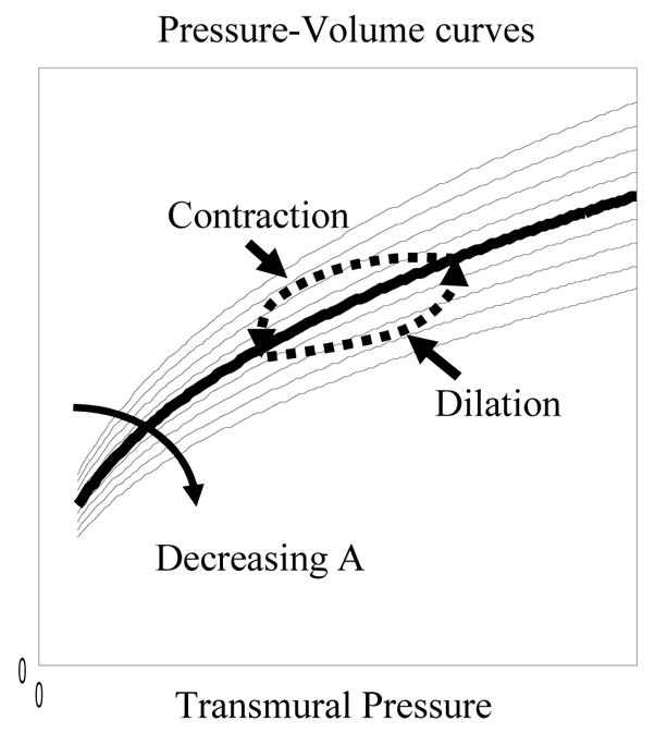
An illustration of the hysteresis loop on a family of steady state pressure-volume (P-V) curves. The hysteresis is the P-V trajectory formed during vessel dilation and contraction.

Another important characteristic of visco-elastic material is that the shape of the hysteresis in the P-V plane is dependent on the rate at which a vessel dilates or contracts. For instance, for slow sinusoidal changes in transmural pressure, hysteresis in the P-V plane almost disappears (Porciuncula et al., 1964) and hence the trajectory of the dynamic P-V curve converges to the steady state P-V curve. Thus the state variable A is dependent on the rate of change of the physical quantities in the system. We selected the following simple first order system to model the state variable A:

$${\tau }_A\frac{dA}{dt}+A=A_{SS}exp\left(-b_0\frac{dV}{dt}\right),b_0>0$$ (3)

where A_SS is the steady state value for A, τ_A is the time constant of the model and b₀ reflects the amount of influence the rate of change in blood volume has on the parameter A.

If the normalised quantities are used: f = F/F₀, v = V/V₀, w = A/A_ss where the subscript 0 denotes baseline values and the subscript ss denotes steady state values, then eqn.s (2) and (3) result in the following VW model:

$$\begin{array}{c}{\tau }_v\frac{dv}{dt}=f-\frac{v^{\phi }}{w}\\ {\tau }_w\frac{dw}{dt}+w=exp\left(-b\frac{dv}{dt}\right)\end{array}$$ (4)

where τ_v is the venous transit time (V₀/F₀), the exponent φ = α + β is a constant, b = b₀V₀ is the gain parameter modelling the degree of influence exerted by $\frac{dv}{dt}$ on w, and τ_w = τ_A is the time constant of w. The state variable w reflects the normalised changes in the muscle tone of blood vessels. The VW model captures several properties of visco-elastic material:

1. At any steady state, $\frac{dv}{dt}=\frac{dw}{dt}=0$, hence w = 1. This preserves the steady state P-V relationship of the blood vessel.

2. During vessel dilation, $\frac{dv}{dt}>0$, hence $exp\left(-b\frac{dv}{dt}\right)<1$ (for b > 0). This implies that w will decrease from its baseline value of unity, resulting in a P-V trajectory ‘below’ the steady state P-V curve during dilation. By the same reasoning, the P-V trajectory during vessel contraction is ‘above’ the steady state curve (Fig. 2), thus generating a hysteresis loop in the P-V plane as that observed by Poiciuncula et al. (1964).

3. The use of the exponential function provides desirable constraints on the range of values of w. As $\frac{dv}{dt}$ ranges from − ∞ to + ∞, the exponential function varies from 0 to + ∞. Since w is modelled as a first order dynamic system driven by a non-negative exponential function, this ensures that w will never become negative. Consequently the parameter A will be guaranteed to lie within the range (0, + ∞), and the P-V trajectories predicted by the model will always lie within the first quadrant of the P-V plane.

Furthermore by clamping w = 1 for all t, the VW model reduces to

$${\tau }_v\frac{dv}{dt}=f-v^{\phi }$$ (5)

This model is often referred to as the simple ‘balloon’ model (Friston et al., 2000; Kong et al., 2004; Zheng et al., 2002), with the parameter φ equal to the inverse Grubb exponent (Grubb et al., 1974). By clamping w = 1, the model effectively assumes that there is no hysteresis in the P-V plane and that the blood vessel has only elastic properties. Hence in this paper we will refer this model as the elastic windkessel (EW) model. The EW model is a special case of the VW model.

Static and dynamic compliances

The compliance of a blood vessel is determined by the amount of volume change per unit change in transmural pressure, and hence is the gradient of the P-V curve. If the curve is nonlinear, the vessel compliance varies at every steady state. During the transient period, the P-V relationship of a blood vessel forms a hysteresis loop in the P-V plane. Based on these observations, we classify the compliance of a blood vessel into two categories: one is static compliance given by the gradient on the steady-state P-V curve (Fig. 3a), the other dynamic compliance given by the gradient along the hysteresis loop in the P-V plane (Fig. 3b). Whereas the static compliance maybe used to model blood vessels with mainly elastic characteristics such that the hysteresis effect is minimum, the dynamic compliance reflects the visco-elastic properties of a blood vessel during dilation and contraction and is dependent on the rate at which it expands or contracts.

Figure 3.

Steady state P-V curves. (a) Static compliance defined as the gradient on the steady state P-V curve. (b) Dynamic compliance defined as the gradient on the hysteresis loop of the P-V trajectory formed during dynamic phases of dilation and contraction.

From the steady state P-V model V = (AP_w)^1/β, it can be shown that the static compliance is given by

$${C_S=\frac{dV}{dP}\mid }_{SS}=\frac{V}{\beta P}$$ (6)

Furthermore using eqn. (3) it can be shown that the dynamic compliance is given by:

$$C_D==\frac{\stackrel{.}{V}}{\stackrel{.}{P}}=\frac{\stackrel{.}{V}{A}^2}{V^{\beta -1}\left(\beta \stackrel{.}{V}A-V\stackrel{.}{A}\right)}$$ (7)

Their normalised forms are

$$c_s=\frac{C_S}{C_{S0}}=\frac{v}{p}=\frac{1}{p^{1-1/\beta }}=\frac{1}{v^{\beta -1}}$$ (8)

and

$$c_d=\frac{C_D}{C_{D0}}=\frac{\beta w^2\stackrel{.}{v}}{v^{\beta -1}\left(\beta w\stackrel{.}{v}-v\stackrel{.}{w}\right)}$$ (9)

respectively. Note that if a blood vessel behaves like (nonlinear) elastic material, there will be little hysteresis in the P-V plane during vessel dilation and contraction, hence the dynamic compliance as expressed above will converge to the static compliance.

Data Analysis

Spectroscopic data were captured at 7.5 Hz and analysed using a path length scaling algorithm, as described in Mayhew et al. (1999). This algorithm used a modified version of the Beer-Lambert Law which included terms of differential path lengths over the range of wavelengths used. The LDF data were captured at 30 Hz and sub-sampled to 7.5 Hz. Baseline values were calculated from the first 8 seconds of each trial, yielding normalised changes in CBV and CBF as v = V/V₀ and f = F/F₀ respectively.

The parameters of the VW model were estimated for each of the five animals and under each of the five stimulation frequencies (1,2,3,4 and 5Hz), with the exception of animal 4 which has only data for four stimulus frequencies (1,2,3 and 5Hz). Hence there are 24 data sets each with 173 data points. Parameter optimisation was carried out using a nonlinear least squares algorithm (Levenberg-Marquardt algorithm, Matlab^™ function “lsqnonlin”). The performance of the VW model was compared with that of the EW model using the following three methods.

1. For each model, we computed the sum of squares of errors (SSE) for each data set:

   $$\mathit{SSE}=\sum _{i=1}^N{\epsilon }_i^2=\sum _{i=1}^N{\left(\widehat{v}-v\right)}_i^2$$ (10)

   where v and v̂ are the measured CBV time series and the model predicted CBV time series respectively, and N is the number of data points used. Then the difference scores for the SSE

   $$\mathrm{\Delta }\mathit{SSE}=\mathit{SSE}(VW)-\mathit{SSE}(EW)$$

   were computed.

2. The corrected Akaike’s information Criterion (AIC_c) was calculated for each model under each condition. This criterion provides a measure of goodness-of-fit of a model to empirical data, and offers a trade-off between model prediction and model complexity. The equation used for the calculation is:

   $$AI{C}_c=Nlog\left(\frac{\mathit{SSE}}{N}\right)+2K+\frac{2K\left(K+1\right)}{N-K-1}$$ (11)

   where K is the number of parameters in the model, including the estimation of the SSE (Burnham and Anderson, 2002). Model selection was determined by the difference scores in AICc between models. Hence using the EW model as the reference model, we computed the difference scores

   $$\mathrm{\Delta }AI{C}_c=AI{C}_c(VW)-AI{C}_c\left(EW\right)$$

3. In order to compare the predictive properties of the EW and the VW models, we re-optimised the 4Hz data with the two compliance model parameters (b and τ_w) clamped at values optimised for the 5Hz data. In other words we optimised the same model parameters φ and τ_v for both models. This was done for each animal, and the model predicted CBV time series were compared.

Results

The VW model shows much improved performance compared to the EW model. Fig. 4 shows the normalised CBV and the VW model predicted CBV, superimposed with the EW model predicted CBV for a representative subject, which clearly illustrates the improvement of model predictions provided by the VW model at higher stimulus frequencies. At lower stimulation frequencies, in this case at 1Hz, the predictions from both models are almost identical because there is little ‘delayed compliance’ in the data.

Figure 4.

Comparison of the EW and VW model predictions of the CBV time series (normalised w.r.t. baseline values). The normalised CBV data (grey trace) is superimposed with the VW model predicted CBV (black broken trace) and the EW model predicted CBV (black trace). The stimulation duration is indicated by the black bar on the time axis. The five data sets are from a representative subject (subject 3) under conditions of different stimulation.

The difference scores for SSE and AIC_c for each animal under each stimulation frequency were calculated. All ΔSSE are negative, except one (animal 5, 1Hz) which has a difference score of zero.. A t-test on the SSE scores showed that the SSE for the VW model are significantly smaller than those of the EW model (p<0.01), hence the VW model is better at predicting the CBV time series.

The Δ AIC_c scores are shown in Table 1. As a rule of thumb, a model is significantly better than other models if the corrected AIC score is at least 10 units lower than those of the other models (Burnham and Anderson, 2002). In 19 out of 24 data sets, Δ AIC_c are negative with a magnitude much bigger than 10. In these cases the VW model is superior than the EW model. For the remaining five data sets, the Δ AIC_c scores are within ± 10, hence the performances of the two models are not significantly different. Note that these five data sets are all from conditions with lower stimulus frequencies: three of them from 1Hz, and one of each from the 2 and 3 Hz conditions.

The two EW model parameters (φ, τ_v) and the four VW model parameters (φ, τ_v,b, τ_w) were optimised for all 24 data sets and their values are displayed as histograms shown in Fig. 5. Also shown in Figure 5 are the means and standard deviations calculated for each histogram. The statistics for panel (f) of Figure 5 were calculated by excluding the outlier. It can be seen that the standard deviations of the two parameters common to both models (φ, τ_v), are smaller for the VW model than for the EW model. However the differences were not significant at the p<0.05 level. The issue of the outliers in the distributions for the two compliance model parameters (b, τ_w) will be addressed in the Discussion section.

Figure 5.

Histograms of model parameters. The mean and the standard deviation of each histogram are displayed inside each subplot. (a) and (b) are histograms of the two parameters associated with the EW model. (c)–(f) are histograms of the four parameters associated with the VW model respectively. In panel (f), the symbol * is used to highlight the fact that these statistics were calculated excluding one outlier.

Fig. 6 shows the normalised CBV data under the 4Hz stimulation frequency, the EW model predicted CBV and that using the VW model but with the compliance parameters (b, τ_w) clamped at their values optimised for the 5Hz stimulation frequency. It can be seen that apart from subject 1, the VW model predictions for the other three subjects are significantly better than the predictions of the EW model. The data for subject 1 showed a large mismatch between the CBF and CBV time series at 5Hz, but only slight difference at 4Hz. Thus clamping the VW model compliance parameters optimised under the 5Hz condition did not produce good predictions for the 4Hz data for this subject.

Figure 6.

Comparison of the EW and VW model predictions of the CBV time series using clamped parameters. The normalised CBV data (grey trace) is superimposed with the VW model predicted CBV (black broken trace) and the EW model predicted CBV (black trace). The four data sets are from four individual subjects (1,2,3 and 5) with 4Hz stimulation frequency. The VW model predictions were obtained by clamping the two compliance model parameters (b, τ_w) at values optimised for the 5Hz condition.

Discussion

Using the Akaike’s Information Criterion, we have shown that the VW model is superior to the EW model, and the two additional model parameters (b, τ_w) improved model predictions during the return-to-baseline phase of the CBV time series.

There was one outlier in the distribution of the parameter τ_w, with a value of τ_w = 33. For this particular data set (2Hz, animal 2), there was little mismatch between the two time series of CBF and CBV, i.e., they returned to baseline at roughly the same rate. A large τ_w means that the state variable w has very slow dynamics, or hardly varies during the time course of the stimulation.

The histogram of the parameter b also highlights some cases in which much larger values of b were necessary in order to capture the data. Closer examination of the associated data revealed that these cases correspond to the time series of CBV remaining elevated throughout the post-stimulation period that the data was collected, while CBF did return to its baseline. The role of the parameter b is to amplify the influence of dv/dt on the state variable w. In these cases, b has to be sufficiently larger to prevent the state variable w from returning to the steady state value of unity.

In summary an important advantage of the VW model over the EW model is that the values of the two compliance model parameters (b, τ_w) capture the variation of the difference between the CBF and the CBV time series as they return to baseline.

Another important feature of the VW model is that it converges to the Grubb’s relationship CBV ∝ CBF^Φ (Grubb et al., 1974) at steady state. The parameter φ in the VW model is the inverse of the Grubb’s exponent Φ. As φ is the summation of the two parameters: α given by the blood vessel resistance-volume relationship, and β given by the P-V curve, and both parameters have different values for different blood vessel types, it means that the Grubb’s exponent is unlikely to be the same across different vascular compartments. Furthermore, during transient phases of vessel dilation and contraction, the relationship between CBF and CBV is a dynamic one which is not simply governed by the power law described by Grubb et al (1974).

The physiological basis of the CBF-CBV mismatch

In deriving the VW model, we have attributed the observed difference between the time series of CBF and CBV to the visco-elastic properties of the blood vessels. This is based on the following reasoning.

During neural activation, dilation in the arterial compartment reduces the vascular resistance and hence blood flow increases. In the venous compartment, the increased flow from upstream increases the pressure inside the blood vessels. Assuming intracranial pressure remains constant during local hyperaemia (by replacement of the CSF), the transmural pressure in the venous compartment will be increased. Because the venous compartment is passive and the venous blood vessels are visco-elastic, the volume of the vessels increases quickly initially due to the elastic component of the vessel walls, but this expansion slows down considerably as the transmural pressure (and hence CBF) reaches a new steady state (Porciuncula et al., 1964). This is the ‘creep loading’ characteristic of a visco-elastic material. This process also occurs when there is a decrease in transmural pressure, hence there is a mismatch between the time series of CBF and CBV during both the inflation and deflation phases. A recent study by Royl et al. (2008) on the effect of elevated intracranial pressure on neurovascular coupling demonstrated that by increasing the intracranial pressure (hence decreasing the transmural pressure) within an activated region of the rat cortex the temporal mismatch between CBF and CBV was reduced. This suggests that transmural pressure plays an important part in the differences between the time courses of CBF and CBV.

Although many optical imaging and MRI studies demonstrated the mismatch between the time series of CBF and CBV, this phenomenon is not always observed (Donahue et al., 2008; Jin et al., 2006). Some studies even showed no measurable changes of CBV in the venous compartment with respect to evoked changes in neural activity (e.g. Hillman et al., 2007; Kim et al., 2007). This inconsistency across laboratories and across studies could be due to different modalities used for measuring the haemodynamic responses and different stimulus types. But this alone may not explain the considerable variability in the published physiological data. It is possible that other physiological mechanisms, such as changes in haematocrit, also affect the observed mismatch. This is still an area of active research.

Comparison with other existing CBF-CBV models

Two other models relating CBF to CBV are often used as part of an effort to establish a model linking changes in neural activity to the BOLD signal measured in fMRI experiments. One is similar to the EW model, except that the time constant τ_v took on different values during blood vessel dilation and constriction (Buxton et al., 2004). This model has been used in modelling and analysis of the BOLD fMRI data (Deneux and Faugeras, 2006; Vakorin et al., 2007; Vazquez et al., 2006). Like the original windkessel model by Mandeville et al. (1999), this model is time varying. A hidden switching function is required to track the sign of the changes of the CBV time series. A further weakness of the ‘Buxton’ model is that it effectively assumes that during vessel dilation, only the elastic response is present (hence the shorter time constant τ_MTT), and during vessel contraction, only the visco-elastic response is present (hence the longer time constant τ_MTT + τ_visco). Data obtained from long stimulation studies (Herman et al., 2008; Kennerley et al., 2005; Kida et al., 2007; Mandeville et al., 1999) show that during stimulation, there are marked differences between the CBF and CBV time series, i.e., typically the CBF reaches a plateau while CBV is still increasing. However for short stimulation studies, this difference in the time series of CBF and CBV may not be observed because there is insufficient time during the onset phase before the return to baseline phase begins. During the return-to-baseline phase of the haemodynamic responses, the initial rate of decrease in CBF and CBV is in fact similar and the dominant observed mismatch between the CBF and CBV time series only occurs later.

To overcome the problem of the hidden switching function (in both the windkessel model and the Buxton’s model), Kong et al. (2004) extended Mandeville’s windkessel model by introducing a new state variable, which was a function of CBV (but not the rate of change of CBV), and captured some of the desired time varying characteristics of the dynamic compliance. This model was nonlinear time-invariant with four model parameters, much the same as the VW model in terms of model complexity. It was also able to predict well the slow return-to-baseline characteristics of the CBV time series. The model was used (Zheng et al., 2005) to develop a multi-compartmental model linking stimulus to the BOLD signal. However, because the model by Kong et al. (2004) was a formal model and not based on the mechanical properties of visco-elastic materials, it was difficult to relate the additional state and the parameters of the model to the known physiology.

In contrast, the VW model presented here is capable of producing both elastic and visco-elastic responses during stimulus onset and cessation because of the introduction of the state variable w which varies in time. The VW model is in the elastic phase when w is close to unity and transforms itself into the visco-elastic phase as w moves away from unity. Hence, there is no need to decide when to ‘manually’ switch to a different time constant. The compliance parameters (b and τ_w) determine the speed of this transformation and by doing so control the degree of the mismatch between the two time series CBF and CBV. Furthermore, the model is capable of predicting physiologically meaningful variables. For instance, from the relationship V = (AP_w)^1/β, we can write the normalised expression V = (AP_w)^1/β, thus predicting the normalised transmural pressure p_w across the vessel wall (assuming, say lamina flow with α = 2). Fig. 7 shows the results of a simulation of the VW model whose parameters were selected as the mean values of their distributions given in Fig. 5. The normalised CBF time series was the driving input to the model, and the model predicted time series of the normalised CBV and transmural pressure were computed. A step increase in CBF was chosen to demonstrate the visco-elastic properties of the VW model: the CBV response showed the creep loading characteristics, and the transmural pressure showed the stress relaxation characteristics of visco-elastic vessels.

Figure 7.

The visco-elastic properties of the VW model using a simulated step change in CBF (dotted trace). The computed CBV response (solid trace) shows creep loading characteristics, and the computed transmural pressure (broken trace) show characteristics of stress relaxation.

In addition, the VW model has the unique feature that both the static and dynamic compliances are emergent properties of the model. Although these compliances are not explicitly used in the VW model, they are important concepts and directly relevant in modelling the brain vasculature and the blood circulation network (Boas et al., 2008; Huppert et al., 2007; Linehan et al., 1986; Ursino et al., 2000). The use of static instead of dynamic compliance implies the assumption that blood vessels are elastic. This assumption may need to be examined when multi-compartment models are used, as the assumption may stand for the arterial compartment, but is less appropriate for the venous compartment.

Nonlinear vs. linear models

The VW model relates the normalised change in CBF to that of CBV. It is constrained by two nonlinear relationships: (1) the steady state relationship between the normalised CBF and CBV which is widely accepted as a power law relationship (Grubb et al., 1974) rather than a linear one, and (2) the steady state pressure-volume curve of blood vessels which is also well known to be nonlinear; with changes in volume diminishing at high transmural pressure. The VW model introduced a further nonlinearity by modelling the state variable w with the term $exp\left(-b\frac{dv}{dt}\right)$ to ensure that within the theoretical range of $\frac{dv}{dt}\in \left(-\infty ,+\infty \right)$, the state variable w is always positive.

On the other hand, many published data showed that the steady state relationship between the amplitude of changes in CBF and CBV is primarily linear (Ito et al., 2003; Ito et al., 2001; Lee et al., 2001; Risberg et al., 1969; Smith et al., 1971). The dynamic relationship between changes in CBF and CBV was explored (Wang et al., 2007) by linearising the modified windkessel model (Kong et al., 2004). They showed that within the range of changes tested (up to 25% change in CBF and 6% change in CBV), the linearised model was adequate at predicting the time series of changes in CBV from the CBF changes. More recently a linear system identification technique was used (Wei et al., 2009) which further demonstrated that changes in CBF and CBV could be modelled by a linear dynamic system. The drawback of such techniques, however, is that the relationships between the model parameters and any physiological and biophysical constructs are unclear.

Limitations of the VW model

The VW model is guided by the mechanical properties of visco-elastic material, independent of the underlying physiological mechanisms coupling haemodynamic changes to evoked changes in neural activity. Its function is to account for the mismatch between the time series of CBF and CBV, not to model the temporal shape of the CBF itself due to evoked neural activity. The model is most suited to relate the time series of changes in CBF and CBV in the venous compartment due either to evoked neural responses or as part of the circulation vascular network. Unlike the venous compartment which can be modelled as a passive leather bag (windkessel), the cerebral arterial network is actively involved in its role as a cerebral auto-regulation mechanism (Kontos, 1981; Paulson et al., 1990). It has been shown that cerebral arteries of certain diameter range will dilate with a drop in perfusion pressure but constrict with an increase in perfusion pressure in order to maintain cerebral blood flow (Kontos et al., 1978). This is in direct contrast to the P-V relationship of blood vessels measured in vitro. Thus the development of arterial models will be needed for detailed multi-compartment modelling of the relationship between changes in blood flow and volume in the cerebral system.

It is also worthwhile noting that the steady state P-V relationship V = (AP)^1/beta; is a qualitative description of the P-V curve of blood vessels rather than an optimal fit to experimental data. It seems appropriate for describing the P-V relationship of a vein (Porciuncula et al., 1964), but other studies showed that the P-V relationship of an arterial blood vessel maybe better described by a sigmoid function (Bergel, 1961; Roy, 1881). Notwithstanding, the strategy of modelling the parameter of the steady state P-V curve can be extended to other forms of P-V relationships.

Conclusion

This paper proposed a novel strategy for modelling the relationship between the CBF and the CBV time series. The strategy is based on the observation that the pressure-volume relationship of a visco-elastic tube at steady state differs from the relationship during transient states of dilation and contraction. The key point of the VW model is that a parameter characterising the steady state P-V curve becomes time varying during transient states, and the model predicted P-V trajectory form a hysteresis loop. This parameter is treated as a state variable and modelled by a simple first order nonlinear dynamic system driven by the rate of change of volume, and the overall model is nonlinear time-invariant.

Although the VW model has two more parameters than the simpler elastic balloon model, based on Akaike’s information criterion, it is superior. The values of these parameters account for the difference between the time series of CBF and CBV, thus capturing the ‘delayed compliance’ phenomenon.

References

- Alexander RS, Edwards WS, Ankeney JL. The Distensibility Characteristics of the Portal Vascular Bed. Circulation Research. 1953;1:271–277. doi: 10.1161/01.res.1.3.271. [DOI] [PubMed] [Google Scholar]
- Bergel DH. The Static Elastic Properties of Arterial Wall. Journal of Physiology-London. 1961;156:445–457. doi: 10.1113/jphysiol.1961.sp006686. [DOI] [PMC free article] [PubMed] [Google Scholar]
- Boas DA, Jones SR, Devor A, Huppert TJ, Dale AM. A vascular anatomical network model of the spatio-temporal response to brain activation. Neuroimage. 2008;40:1116–1129. doi: 10.1016/j.neuroimage.2007.12.061. [DOI] [PMC free article] [PubMed] [Google Scholar]
- Burnham KP, Anderson DR. Model Selection and Multimodel Inference. 2. Springer; 2002. [Google Scholar]
- Buxton RB, Uludag K, Dubowitz DJ, Liu TT. Modeling the hemodynamic response to brain activation. Neuroimage. 2004;23:S220–S233. doi: 10.1016/j.neuroimage.2004.07.013. [DOI] [PubMed] [Google Scholar]
- Buxton RB, Wong EC, Frank LR. Dynamics of blood flow and oxygenation changes during brain activation: The balloon model. Magnetic Resonance in Medicine. 1998;39:855–864. doi: 10.1002/mrm.1910390602. [DOI] [PubMed] [Google Scholar]
- Deneux T, Faugeras O. Using nonlinear models in fMRI data analysis: Model selection and activation detection. Neuroimage. 2006;32:1669–1689. doi: 10.1016/j.neuroimage.2006.03.006. [DOI] [PubMed] [Google Scholar]
- Donahue MJ, Stevens RD, de Boorder M, Pekar JJ, Hendrikse J, van Zijl PCM. Hemodynamic changes after visual stimulation and breath holding provide evidence for an uncoupling of cerebral blood flow and volume from oxygen metabolism. Journal of Cerebral Blood Flow and Metabolism. 2008;29:176–185. doi: 10.1038/jcbfm.2008.109. [DOI] [PMC free article] [PubMed] [Google Scholar]
- Fogliardi R, Di Donfrancesco M, Burattini R. Comparison of linear and nonlinear formulations of the three-element windkessel model. American Journal of Physiology-Heart and Circulatory Physiology. 1996;40:H2661–H2668. doi: 10.1152/ajpheart.1996.271.6.H2661. [DOI] [PubMed] [Google Scholar]
- Frank O. Evaluation of the shock volume of the human heat on the basis of waves and Windkessel theory. Zeitschrift fur Biologie. 1930;90:405–409. [Google Scholar]
- Friston KJ, Mechelli A, Turner R, Price CJ. Nonlinear responses in fMRI: The balloon model, volterra kernels, and other hemodynamics. Neuroimage. 2000;12:466–477. doi: 10.1006/nimg.2000.0630. [DOI] [PubMed] [Google Scholar]
- Grubb RL, Raichle ME, Eichling JO, Terpogos Mm. Effects of Changes in Paco2 on Cerebral Blood Volume, Blood Flow, and Vascular Mean Transit Time. Stroke. 1974;5:630–639. doi: 10.1161/01.str.5.5.630. [DOI] [PubMed] [Google Scholar]
- Herman P, Sanganahalli BG, Hyder F. Multimodal measurements of blood plasma and red blood cell volumes during functional brain activation. Journal of Cerebral Blood Flow and Metabolism. 2008;29:19–24. doi: 10.1038/jcbfm.2008.100. [DOI] [PMC free article] [PubMed] [Google Scholar]
- Hillman EMC, Devor A, Bouchard MB, Dunn AK, Krauss GW, Skoch J, Bacskai BJ, Dale AM, Boas DA. Depth-resolved optical imaging and microscopy of vascular compartment dynamics during somatosensory stimulation. Neuroimage. 2007;35:89–104. doi: 10.1016/j.neuroimage.2006.11.032. [DOI] [PMC free article] [PubMed] [Google Scholar]
- Huppert TJ, Allen MS, Benav H, Jones PB, Boas DA. A multicompartment vascular model for inferring baseline and functional changes in cerebral oxygen metabolism and arterial dilation. Journal of Cerebral Blood Flow and Metabolism. 2007;27:1262–1279. doi: 10.1038/sj.jcbfm.9600435. [DOI] [PMC free article] [PubMed] [Google Scholar]
- Ito H, Kanno I, Ibaraki M, Hatazawa J, Miura S. Changes in human cerebral blood flow and cerebral blood volume during hypercapnia and hypocapnia measured by positron emission tomography. Journal of Cerebral Blood Flow and Metabolism. 2003;23:665–670. doi: 10.1097/01.WCB.0000067721.64998.F5. [DOI] [PubMed] [Google Scholar]
- Ito H, Takahashi K, Hatazawa J, Kim SG, Kanno I. Changes in Human Regional Cerebral Blood Flow and Cerebral Blood Volume During Visual Stimulation Measured by Positron Emission Tomography. Journal of Cerebral Blood Flow and Metabolism. 2001;21:608–612. doi: 10.1097/00004647-200105000-00015. [DOI] [PubMed] [Google Scholar]
- Jin T, Wang T, Zhao F, Wang P, Tasker M, Kim S-G. Spatiotemporal characteristics of BOLD, CBV and CBF responses in the cat visual cortex. Proc Intl Soc Mag Reson Med. 2006;14:2762. [Google Scholar]
- Jones M, Berwick J, Johnston D, Mayhew J. Concurrent optical imaging spectroscopy and laser-Doppler Flowmetry: The relationship between blood flow, oxygenation, and volume in rodent barrel cortex. Neuroimage. 2001;13:1002–1015. doi: 10.1006/nimg.2001.0808. [DOI] [PubMed] [Google Scholar]
- Jones M, Berwick J, Mayhew J. Changes in blood flow, oxygenation, and volume following extended stimulation of rodent barrel cortex. Neuroimage. 2002;15:474–487. doi: 10.1006/nimg.2001.1000. [DOI] [PubMed] [Google Scholar]
- Jones RT. Blood Flow. Annual Review of Fluid Mechanics. 1969;1:223–244. [Google Scholar]
- Kennerley AJ, Berwick J, Martindale J, Johnston D, Papadakis N, Mayhew J. Concurrent fMRI and Optical Measures for the Investigation of the Hemodynamic Response Function. MRM. 2005;54:354–365. doi: 10.1002/mrm.20511. [DOI] [PubMed] [Google Scholar]
- Kida I, Rothman DL, Hyder F. Dynamics of changes in blood flow, volume, and oxygenation: implications for dynamic functional magnetic resonance imaging calibration. Journal of Cerebral Blood Flow and Metabolism. 2007;27:690–696. doi: 10.1038/sj.jcbfm.9600409. [DOI] [PMC free article] [PubMed] [Google Scholar]
- Kim T, Hendrich KS, Masamoto K, Kim SG. Arterial versus total blood volume changes during neural activity-induced cerebral blood flow change: implication for BOLD fMRI. Journal of Cerebral Blood Flow and Metabolism. 2007;27:1235–1247. doi: 10.1038/sj.jcbfm.9600429. [DOI] [PubMed] [Google Scholar]
- Klabunde RE. Cardiovascular Physiology Concepts. Lippincott Williams & Wilkins; US: 2005. [Google Scholar]
- Kong YZ, Zheng Y, Johnston D, Martindale J, Jones T, Billings S, Mayhew T. A model of the dynamic relationship between blood flow and volume changes during brain activation. Journal of Cerebral Blood Flow and Metabolism. 2004;24:1382–1392. doi: 10.1097/01.WCB.0000141500.74439.53. [DOI] [PubMed] [Google Scholar]
- Kontos HA. Regulation of the Cerebral-Circulation. Annual Review of Physiology. 1981;43:397–407. doi: 10.1146/annurev.ph.43.030181.002145. [DOI] [PubMed] [Google Scholar]
- Kontos HA, Wei EP, Navari RM, Levasseur JE, Rosenblum WI, Patterson JL. Responses of Cerebral-Arteries and Arterioles to Acute Hypotension and Hypertension. American Journal of Physiology. 1978;234:H371–H383. doi: 10.1152/ajpheart.1978.234.4.H371. [DOI] [PubMed] [Google Scholar]
- Lee SP, Duong TQ, Yang G, Iadecola C, Kim SG. Relative changes of cerebral arterial and venous blood volumes during increased cerebral blood flow: Implications for BOLD fMRI. Magnetic Resonance in Medicine. 2001;45:791–800. doi: 10.1002/mrm.1107. [DOI] [PubMed] [Google Scholar]
- Linehan JH, Dawson CA, Rickaby DA, Bronikowski TA. Pulmonary Vascular Compliance and Viscoelasticity. Journal of Applied Physiology. 1986;61:1802–1814. doi: 10.1152/jappl.1986.61.5.1802. [DOI] [PubMed] [Google Scholar]
- Mandeville JB, Marota JJA, Ayata C, Zaharchuk G, Moskowitz MA, Rosen BR, Weisskoff RM. Evidence of a cerebrovascular postarteriole windkessel with delayed compliance. Journal of Cerebral Blood Flow and Metabolism. 1999;19:679–689. doi: 10.1097/00004647-199906000-00012. [DOI] [PubMed] [Google Scholar]
- Martindale J, Mayhew J, Berwick J, Jones M, Martin C, Johnston D, Redgrave P, Zheng Y. The hemodynamic impulse response to a single neural event. Journal of Cerebral Blood Flow and Metabolism. 2003;23:546–555. doi: 10.1097/01.WCB.0000058871.46954.2B. [DOI] [PubMed] [Google Scholar]
- Mayhew J, Zheng Y, Hou YQ, Vuksanovic B, Berwick J, Askew S, Coffey P. Spectroscopic analysis of changes in remitted illumination: The response to increased neural activity in brain. Neuroimage. 1999;10:304–326. doi: 10.1006/nimg.1999.0460. [DOI] [PubMed] [Google Scholar]
- Molino P, Cerutti C, Julien C, Cuisinaud G, Gustin MP, Paultre C. Beat-to-beat estimation of windkessel model parameters in conscious rats. American Journal of Physiology-Heart and Circulatory Physiology. 1998;43:H171–H177. doi: 10.1152/ajpheart.1998.274.1.H171. [DOI] [PubMed] [Google Scholar]
- Nilsson GE. Signal Processor for Laser Doppler Tissue Flowmeters. Medical and Biological Engineering and Computing. 1984;22:343–348. doi: 10.1007/BF02442104. [DOI] [PubMed] [Google Scholar]
- Orosz M, Molnarka G, Toth M, Nadasy GL, Monos E. Viscoelastic behavior of vascular wall simulated by generalized Maxwell models - a comparative study. Medical Science Monitor. 1999;5:549–555. [Google Scholar]
- Paulson OB, Strandgaard S, Edvinsson L. Cerebral Autoregulation. Cerebrovascular and Brain Metabolism Reviews. 1990;2:161–192. [PubMed] [Google Scholar]
- Porciuncula CI, Armstrong GG, Stone HL, Guyton AC. Delayed Compliance in External Jugular Vein Ofdog. American Journal of Physiology. 1964;207:728–732. doi: 10.1152/ajplegacy.1964.207.3.728. [DOI] [PubMed] [Google Scholar]
- Remington JW, Alexander RS. Stretch Behavior of the Bladder as an Approach to Vascular Distensibility. American Journal of Physiology. 1955;181:240–248. doi: 10.1152/ajplegacy.1955.181.2.240. [DOI] [PubMed] [Google Scholar]
- Risberg J, Ancri D, Ingvar DH. Correlation between cerebral blood volume and cerebral blood flow in the cat. Experimental Brain Research. 1969;8:321–326. doi: 10.1007/BF00234379. [DOI] [PubMed] [Google Scholar]
- Roy CS. The elastic properties of the arterial wall. J Physiol. 1881;3:125–159. doi: 10.1113/jphysiol.1881.sp000088. [DOI] [PMC free article] [PubMed] [Google Scholar]
- Royl G, Fuchtemeier M, Leithner C, Kohl-Bareis M, Dirnagl U, Lindauer U. Influence of intracranial pressure on neurovascular coupling: clarifying mechanisms of the BOLD post-stimulus undershoot. Society for Neuroscience. 2008 Abstract 482.6. [Google Scholar]
- Segers P, Rietzschel ER, De Buyzere ML, Stergiopulos N, Westerhof N, Van Bortel LM, Gillebert T, Verdonck PR. Three- and four-element Windkessel models: assessment of their fitting performance in a large cohort of healthy middle-aged individuals. Proceedings of the Institution of Mechanical Engineers Part H-Journal of Engineering in Medicine. 2008;222:417–428. doi: 10.1243/09544119JEIM287. [DOI] [PubMed] [Google Scholar]
- Smith AL, Neufeld GR, Ominsky AJ, Wollman H. Effect of arterial CO 2 tension on cerebral blood flow, mean transit time, and vascular volume. Journal of Applied Physiology. 1971;31:701–707. doi: 10.1152/jappl.1971.31.5.701. [DOI] [PubMed] [Google Scholar]
- Stergiopulos N, Westerhof BE, Westerhof N. Total arterial inertance as the fourth element of the windkessel model. American Journal of Physiology-Heart and Circulatory Physiology. 1999;276:H81–H88. doi: 10.1152/ajpheart.1999.276.1.H81. [DOI] [PubMed] [Google Scholar]
- Ursino M, Ter Minassian A, Lodi CA, Beydon L. Cerebral hemodynamics during arterial and CO2 pressure changes: in vivo prediction by a mathematical model. American Journal of Physiology-Heart and Circulatory Physiology. 2000;279:H2439–H2455. doi: 10.1152/ajpheart.2000.279.5.H2439. [DOI] [PubMed] [Google Scholar]
- Vakorin VA, Krakovska OO, Borowsky R, Sarty GE. Inferring neural activity from BOLD signals through nonlinear optimization. Neuroimage. 2007;38:248–260. doi: 10.1016/j.neuroimage.2007.06.033. [DOI] [PubMed] [Google Scholar]
- Vazquez AL, Cohen ER, Gulani V, Hernandez-Garcia L, Zheng Y, Lee GR, Kim SG, Grotberg JB, Noll DC. Vascular dynamics and BOLD fMRI: CBF level effects and analysis considerations. Neuroimage. 2006;32:1642–1655. doi: 10.1016/j.neuroimage.2006.04.195. [DOI] [PubMed] [Google Scholar]
- Wang KY, Zheng Y, Billings S, Coca D, Johnston D, Mayhew J. Estimating CBF changes from measurements of CBV changes: a linear dynamic modelling approach. Society for Neuroscience 2007. 2007 Abstract 753.17. [Google Scholar]
- Wei HL, Zheng Y, Pan Y, Coca D, Li LM, Mayhew J, Billings S. Model estimation of cerebral hemodynamics between blood flow and volume changes: A data-based modelling approach. IEEE Trans Biomedical Engineering. 2009 doi: 10.1109/TBME.2009.2012722. In press. [DOI] [PubMed] [Google Scholar]
- Westerhof N, Elzinga G, Sipkema P. An Artificial Arterial System for Pumping Hearts. Journal of Applied Physiology. 1971;31:776–781. doi: 10.1152/jappl.1971.31.5.776. [DOI] [PubMed] [Google Scholar]
- Zheng Y, Johnston D, Berwick J, Chen DM, Billings S, Mayhew J. A three-compartment model of the hemodynamic response and oxygen delivery to brain. Neuroimage. 2005;28:925–939. doi: 10.1016/j.neuroimage.2005.06.042. [DOI] [PubMed] [Google Scholar]
- Zheng Y, Martindale J, Johnston D, Jones M, Berwick J, Mayhew J. A model of the Hemodynamic response and oxygen delivery to brain. Neuroimage. 2002;16:617–637. doi: 10.1006/nimg.2002.1078. [DOI] [PubMed] [Google Scholar]