

Summary
Quantitatively describing RNA structure and conformational elements remains a formidable problem. Seven standard torsion angles and the sugar pucker are necessary to completely characterize the conformation of an RNA nucleotide. Progress has been made toward understanding the discrete nature of RNA structure, but classifying simple and ubiquitous structural elements such as helices and motifs remains a difficult task. One approach for describing RNA structure in a simple, mathematically consistent, and computationally accessible manner involves the invocation of two pseudotorsions, η (C4’n-1, Pn, C4’n, Pn+1) and θ (Pn, C4’n, Pn+1, C4’n+1), which can be used to describe RNA conformation in much the same way that ϕ and ψ are used to describe backbone configuration of proteins. Here we conduct an exploration and statistical evaluation of pseudotorsional space and of the Ramachandran-like η−θ plot. We show that, through the rigorous quantitative analysis of the η−θ plot, the pseudotorsional descriptors η and θ, together with sugar pucker, are sufficient to describe RNA backbone conformation fully in most cases. These descriptors are also shown to contain considerable information about nucleotide base conformation, revealing a previously uncharacterized interplay between backbone and base orientation. A window function analysis is used to discern statistically relevant regions of density in the η−θ scatter plot and then nucleotides in colocalized clusters in the η−θ plane are shown to have similar three-dimensional structures through RMSD analysis of the RNA structural constituents. We find that major clusters in the η−θ plot are few in number, thereby underscoring the discrete nature of RNA backbone conformation. Like the Ramachandran plot, the η−θ plot is a valuable system for conceptualizing biomolecular conformation, it is a useful tool for analyzing RNA tertiary structures, and it is a vital component of new approaches for solving the three-dimensional structures of large RNA molecules and RNA assemblies.
Keywords: RNA structure, reduced representation, pseudotorsions, Ramachandran, cluster analysis
Introduction
Describing and manipulating RNA structure is a spatially complex problem because six standardized torsion angles (α, β, γ, δ, ε, and ζ) are required to specify the backbone conformation of a single nucleotide. It is difficult to use these standard torsions for classifying RNA structural motifs, such as helices, because of the “crankshaft effect” 1; 2, in which large changes in individual torsion angles are compensated by changes in other torsion angles. As a result, diverse combinations of standard torsion angles can describe identical nucleotide morphologies, even for the simplest motifs such as short duplexes.
It has recently been shown that RNA backbone morphologies and standard torsion angles fall into discrete categories 3-5. Although these observations significantly enhance our understanding of RNA structure, their application involves the use of six-dimensional or larger spaces, resulting in a complexity that belies the inherent conformational simplicity of many RNA structures, such as helices and tetraloops. It would be beneficial to complement these efforts with a simple approach such as that employed for proteins, in which two torsion angles, φ and ψ, readily distinguish important amino acid conformations in motifs such as α-helices and β-sheets.
Alternative descriptions of RNA structure can address many of these issues and simplify the problem of RNA conformational space. Attempts have been made to construct reduced representations of RNA structure 6-9. For the most part, these methods have been used for modeling global architecture rather than a description of conformation at the nucleotide level. Previous work has established that a specific set of pseudotorsion angles can serve as descriptors of RNA nucleotide conformation, and that they can distinguish many discrete nucleotide morphologies and structural motifs.6 Using this convention, RNA is characterized in a heuristic but quantitative manner by reducing the nucleotide backbone to two imaginary torsion angles that result from pseudobonds connecting C4’ to P atoms:6; 10; 11, η (C4’n-1, Pn, C4’n, Pn+1) and θ (Pn, C4’n, Pn+1, C4’n+1)(Figure 1). By plotting θ vs. η values for nucleotides in a structural database, one obtains a Ramachandran-like scatter plot 12 that displays clustering of nucleotides with similar conformation. However, at the time of the original work, the database of solved RNA structures was not large enough to analyze with statistical confidence. Over the last few years the database has matured considerably, highlighted by the crystallization of ribosomal structures 13 and other ribozymes 14. A quantitative assessment of pseudotorsional descriptors and their inherent information content has now become feasible.
Figure 1.
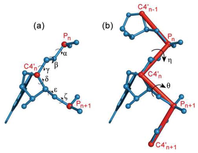
(a) Diagram of a nucleotide showing the standard backbone torsional angles. (b) Diagram depicting the definitions of the pseudotorsions, η and θ. The red lines indicate the pseudo-bonds that connect successive P and C4’ atoms. The portion of the backbone shown is that which affects a single pair of η and θ values, as the pseudotorsions extend into the previous and next nucleotide. In both diagrams, the P and C4’ atoms are shown in red and labeled for reference.
Here we demonstrate that η and θ are robust descriptors of RNA structure and that the information lost in this reduced representation is minimal. The η−θ plot is shown to be statistically non-uniform, and confined regions of the plot are demonstrated to have a higher density of points than the plot average. The identification and spatial parameterization of these high density regions is accomplished through the application of a window function. RMSD superposition of nucleotides within regions of the plot shows that these nucleotides are almost identical. Importantly, the analysis reveals that inclusion of sugar pucker conformation enables one to define nucleotide conformation completely, so the two dominant RNA sugar puckers (C2’-endo and C3’-endo) are treated separately.
Here we show that, for many applications, only two atoms in the backbone are necessary for describing nucleotide backbone conformation. Indeed, specific motifs and strands of nucleotides can be accurately built using only pseudotorsional information. Although we originally undertook this study in order to quantitatively assess the validity of RNA pseudotorsional space, the analysis has revealed new insights into RNA conformational behavior. By showing that there are only a small number of discrete, highly populated clusters in η−θ space, we demonstrate that the number of preferred RNA conformations is limited. We show that nucleobase position is tightly linked to, and can usually be predicted by, metrics that only describe backbone configuration. Taken together, these approaches provide evidence that RNA morphology, including base plane orientation, can often be characterized by simple representations such as the backbone pseudotorsion angles η and θ.
Results
As a starting point for evaluating the precision of pseudotorsions as nucleotide descriptors, the η and θ values for each RNA nucleotide within the complete data set of available high resolution crystal structures were plotted against each other on a two dimensional scatter plot (Figure 2(a)). Each point of the resulting plot represents the η−θ coordinates for a particular nucleotide in the collective database.
Figure 2.
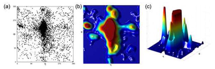
The effect of windowing an η−θ plot with a Blackman window function of width 60°. (a) An η−θ scatter plot of all nucleotides from our data set. Each point shows the η and θ values of an individual nucleotide. (b) The result of applying the Blackman window to the data set, colored from low to high density: blue, green, yellow, and red. (c) A 3-dimensional representation of the data set with a Blackman window function applied. An upper cutoff has been applied to allow for better discerning of the peaks surrounding the helical region.
Once the plot was created, it was important to establish whether sets of points fall within the same region of space, much as they do in a protein Ramachandran plot. Visual inspection indicates that most areas of the η−θ plot contain at least a few points, reflecting the extreme diversity in conformation of RNA nucleotides. However, it is also evident that the plot contains densely populated regions, where a region is operationally defined as an isolated area of the plot with high or low density compared to the average density (ρ̄) of points in the plot. Many of the high density regions in the plot correspond with those previously (and approximately) elucidated 6, although new regions have emerged as well. According to the Kolmogorov-Smirnov statistical test 15, the probability that the distribution of points in the η−θ plot is uniform is exceedingly small (p~10-19), thereby providing a global metric for the notion that the η−θ plot contains areas of high and low density.
Although high density regions were visually detectable, they had not been statistically validated, their boundaries were not specified, and it was not yet known if the regions constitute functional clusters, where a cluster is operationally defined as a high density region that contains a large number of structurally identical nucleotides. The existence of clusters would support the notion that η and θ can uniquely characterize nucleotide conformation.
Application of a window function for rigorous regional specification
To rigorously specify high density regions of the plot and to establish their boundaries, we employed data windowing (kernel smoothing or kernel density estimation) 16, which transforms the η−θ scatter plot into a density plot (Figure 2(a,b)). This method is commonly employed in astronomy to determine the density of matter at a given location in outer space 17. Applying a window function to the data assigns to every point a score that corresponds to the population of its neighborhood.
Data windowing adds a third dimension to the η−θ plot that is proportional to regional density (Figure 2(c)). Areas that contain numerous data points are displayed with large density values, and areas relatively devoid of points exhibit proportionally lower values. For example, applying a window function to a uniform plot would result in a smooth landscape, while a plot with confined and isolated high density regions should yield a plot with pronounced peaks and valleys. The peak shapes and sizes are determined by the shape and width of the window function that is employed.
The Blackman window function 18 was chosen for our analysis of the η−θ plot. Each type of window function tends to have its advantages and drawbacks. Some window functions, like the Gaussian, can be expensive computationally. Others, such as the top hat, are efficient but can artificially overemphasize small scale features of the plot 15. The Blackman window function is efficient to implement and yields very good gradient reproduction 19. That is, the slope of the 3-dimensional density plot at a given point is accurate. The Blackman window provides a good balance between the efficiency of the top hat and the accuracy of smooth window functions like the Gaussian.
For preliminary analysis, the η−θ plot of all nucleotides in the data set was passed through a Blackman window with a width roughly the size of the apparent regions (60°). Many high density regions immediately became apparent (Figure 2(b)), reinforcing the observation that the plot was non-uniform. It also suggested that the η−θ plot represents a map of discrete RNA conformations.
We sought to identify regions with density significantly above the average density of the plot. Applying the Blackman window to the scatter plot yielded a plot with a density value at every point, and the average density (ρ̄) and standard deviation (σ) were calculated. Regions were defined as contiguous areas of the plot with density at least 1σ above average. The nucleotides whose η−θ values fell inside a region were defined as the region’s constituents. This methodology can be understood 3-dimensionally (Figure 2(c)). The z-axis corresponds to density, and the statistically significant parts of the plot are the areas that have densities larger than z = ρ̄ + 1σ.
A global correlation between small RMSD values and similar η−θ coordinates
If a set of η and θ coordinates are good conformational descriptors, then they should uniquely specify local nucleotide geometry with little or no degeneracy. In other words, two nucleotides with widely differing η−θ coordinates should deviate markedly in conformation, while those with similar η−θ coordinates should look alike. By superimposing two RNA substructures with similar η and θ coordinates and then calculating the RMSD between them, one can quantitatively assess their relative degree of conformational similarity.
The correlation between structural similarity (by RMSD) and colocalization of η−θ coordinates was first examined in a global fashion. Random pairs of nucleotides were chosen from the complete data set of RNA structures (see Methods). After calculating their respective position in the η−θ plane, the residue pairs were superimposed and their RMSD values were determined. Initially, only the backbone atoms were considered (Figure 3a). This reveals a striking linear relationship between RMSD and distance apart in the η−θ plane (R2 = 0.80, p ≪ 0.001, see Methods). A notable feature of the graph is that two nucleotides with almost identical η−θ coordinates have backbone RMSD values that are always less than 0.5 Å. Furthermore, large RMSD values are observed only for nucleotides that are far apart in the η−θ plane. For comparison purposes, the equivalent relationship was calculated using the standard torsions in place of the pseudotorsions (Figure 3c). A linear relationship is still apparent (R2 = 0.50, p ≪ 0.001), but it is significantly weaker than when using η and θ. It is interesting that the standard torsions also correlate quite closely to RMSD at values below 0.5 Å, but at higher RMSD values, even slight variations in the structure can lead to vastly differing torsional angles. This is in contrast to the pseudotorsions, where the linear relationship still holds at these higher RMSD values.
Figure 3.
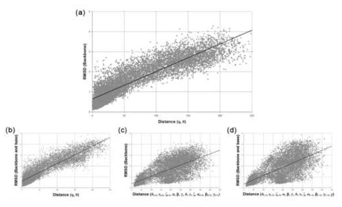
Scatter plots of RMSD versus distance in the η−θ plane or standard torsional angles for 10,000 random pairs of nucleotides from the data set. For each plot, the best fit line is shown on the plot. (a) RMSD of backbone atoms versus distance in the η-θ plane. The correlation coefficient is 0.80. (b) RMSD of backbone atoms versus distance of standard torsional backbone angles. The correlation coefficient is 0.50. (c) RMSD of backbone, sugar, and base atoms versus distance in the η-θ plane. The correlation coefficient is 0.81. (d) RMSD of backbone, sugar, and base atoms versus distance of the standard torsional angles (including χ). The correlation coefficient is 0.50.
To examine the relationship between pseudotorsion angles and base position, the global RMSD analysis was repeated using both the backbone and base atoms for calculating RMSD (see Methods). The resulting correlation between pseudotorsions and RMSD (R2 = 0.81, p ≪ 0.001, Figure 3b) is stronger than that between pseudotorsions and backbone RMSD, although not significantly (p = .039). Finally, we calculated the relationship between backbone and base RMSD for the standard torsions, including the χ angle (Figure 3d). As before, a linear relationship between standard torsions and RMSD is only vaguely apparent (R2 = 0.50, p ≪ 0.001). When the χ angle is not considered, the correlation is slightly weaker (R2 =0.49, p ≪ 0.001, data not shown). These global results imply that the ability of η and θ to distinguish conformation can be comparable to a full set of atomic backbone coordinates.
Using RMSD to evaluate structural similarity within regions of the η−θ plot
RMSD superpositions were then used to quantitatively and unambiguously determine whether regions of the η−θ plot contain conformationally similar groupings of nucleotides (i.e. whether they were bona-fide structural “clusters”). This “cluster analysis” was conducted in several stages: First, the Blackman window function was applied to the plot in order to find regions with high density. To elucidate regions, various density plots were made, each of which showed only areas with density higher than a specific statistically significant value (e.g. ρ̄ + 1σ, ρ̄ + 2σ, ρ̄ + 3σ, etc.). The resultant contiguous regions in each plot were scored by the RMSD values of their components. Specifically, RMSD values were calculated for all pairs of nucleotides in a region, and a “representative” or “prototypical” nucleotide was determined as the nucleotide that looked the most like the others from the region (i.e. the nucleotide with the lowest average RMSD to the others; see Methods for details). The regional score was calculated as the percentage of nucleotides that superimposed with low RMSD (≤ 0.95Å) relative to the prototype. For example, 90% of the nucleotides in a region with a score of 90 are determined by RMSD to be nearly identical to the prototype (see Methods) and therefore form a group of nucleotides with similar morphology. A cluster was then operationally defined as a high density region with a minimum score of 70. This scoring process was repeated for each of the regions. A contour plot was then constructed by compiling the results for the various levels of density. It is important to note that all regions were automatically scored based on all of their constituents and the data set was not manipulated or filtered in any way before analysis.
The sugar pucker problem and subsequent division of the data set
Cluster analysis of the plot revealed that η-θ coordinates are not always able to distinguish between nucleotides with different sugar pucker conformations. The contour plot derived from the entire data set reveals six clusters, most of which have strikingly high scores (80+, data not shown). However, two of these clusters have low scores and, when analyzed individually, they were each found to represent a combination of two distinct conformational subpopulations. Interestingly, the subpopulations were found to differ in sugar pucker conformation. One group consists of nucleotides with C3’-endo sugar pucker (“C3’-endo nucleotides”), while the other has nucleotides with C2’-endo sugar pucker (“C2’-endo nucleotides”).
The simplest solution to the sugar pucker problem was to include sugar pucker conformation as a third parameter. Since RNA nucleotides generally adopt only two sugar pucker conformations (C3’-endo and C2’-endo) 20, the data set was likewise divided into two sets (C3’-endo nucleotides and C2’-endo nucleotides). C3’-endo and C2’-endo nucleotides comprise 82% and 10% of the data set, respectively. Nucleotides with other sugar puckers are very few in number, they are usually close in conformation to the major C2’- and C3’-endo classes and are not considered further here.
An η−θ plot of C3’-endo nucleotides revealed a large, highly populated region near its center. This region contains helical nucleotides and has a density that is almost two orders of magnitude larger than any other, effectively dwarfing the regions that surrounded it. To study the surrounding regions with precision, we effectively subtracted the helical region by separating the set of C3’-endo nucleotides into helical and non-helical nucleotides (see Methods). Separate η−θ plots were then constructed for the three sets: non-helical C3’-endo nucleotides, helical C3’-endo nucleotides, and all C2’-endo nucleotides. Clustered groupings in the individual plots were then examined for conformational similarity.
Results for non-helical C3’-endo nucleotides
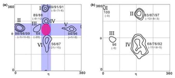
The window function was first applied to the plot of non-helical C3’-endo nucleotides (Figure 4(a)), resulting in a characteristic density profile (Figure 4(b)). A contour plot (Figure 4(c)) was then created by scoring density plots with three different minimum densities: ρ̄ + 1σ, ρ̄ + 2σ, and ρ̄ + 4σ and compiling the results. Strikingly, all of the significant regions have scores of 75 or higher and predominantly contain identical nucleotide conformers. The large proportion of high scores indicates that the clusters in the η−θ plot are indeed meaningful conformational groupings.
Figure 4.
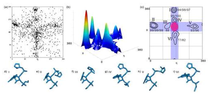
Cluster analysis of the plot of non-helical C3’-endo nucleotides. (a) A scatter plot of the η−θ values of all C3’-endo nucleotides. (b) A 3-dimensional view of the plot of C3’-endo nucleotides with a 60° wide Blackman window function applied. (c) A contour plot and the results of analyzing the density plot. Contour levels are shown for ρ̄ + 1σ, ρ̄ + 2σ, and ρ̄ + 4σ, and scores are given in that order. Contours with small populations (<9) are not shown. The blue bars span the helical η values and the helical θ values. The pink, elliptical area near the center of plot indicates the helical region and was initially excluded from the analysis. (d-i) Prototype nucleotides corresponding to the clusters labeled in (c). Portions of the previous and next nucleotide that affect the pseudotorsions are also shown.
It is notable that many clusters have either helical η or helical θ values (or both), as indicated by the blue highlighted areas of Figure 4(c). These findings indicate that non-helical C3’-endo nucleotides usually initiate or terminate helical strands. The base planes of C3’-endo nucleotides typically stack with at least one neighbor and are unlikely to be splayed out. Also notable was a lack of nucleotides that can be characterized by η−θ coordinates located in the corners of the plot (Figure 4(c)). No clusters were found in these corner areas, suggesting the possibility of generally forbidden areas in the plot. Despite the absence of clusters, the corner areas are not completely devoid of nucleotides. However, these nucleotides have highly unusual conformations that are often characterized by highly splayed base planes, and they do not form stacking interactions with their 5’ or 3’ neighbors.
It is interesting to consider the structural composition of robust clusters that were identified by this methodology. Five of the six C3’-endo clusters contain constituents of known structural motifs. Interestingly, some of the clusters correspond to those previously identified in the 1998 AMIGOS analysis6 (clusters II, V, and VI), while others are new (clusters I, III, and IV).
C3’-endo Cluster I
This cluster appears to have emerged as a direct consequence of the new ribosomal structures. That is, many of the nucleotides in this cluster are constituents of S1 and S2 motifs 21; 22, which are typically found in the ribosome. The η-value for a nucleotide in this cluster is typical for a helical nucleotide, but the θ-value for nucleotides in this cluster is ~120° from helical. This cluster contains nucleotides that stack with both their 5’ and 3’ neighbors, but stacking on the 3’ side is accommodated by the fact that the 3’ neighbors consistently have C2’-endo sugar puckers (for example, 1S7223 0:C586).
C3’-endo Cluster II
Almost all of the nucleotides in this cluster are structurally identical. This cluster, which was previously reported as the stacked turn region 6, contains nucleotides that often serve as the second bases in GNRA or GNRA-like tetraloops and, less frequently, in T-loop motifs. Characteristic of these nucleotides are helical-like θ-values and very non-helical η-values that are on average 140° from helical. They exhibit a sharp backbone kink on their 5’ sides and do not participate in same strand stacking on their 5’ sides (for example, 1S7223 0:C1810). Strikingly, nearly all of these nucleotides are similar in both backbone and structural context.
C3’-endo Cluster III
Nucleotides in this cluster have θ-values that match those of helical nucleotides but η-values that are smaller than helical and range from 99° to 143°. These residues are frequently preceded on the 5’-side by nucleotides with C2’-endo sugar pucker. Consequently, there is an almost “zig-zag” like bend in the backbone (see Figure 4(f)). Nucleotides belonging to this cluster often comprise the 3’ halves of adenosine platforms and similar structures 24 (for example, 1S7223 0:U2650).
C3’-endo Cluster IV
Like cluster III, cluster IV sits close to the helical region. Nucleotides in cluster IV have helical η-values and non-helical θ-values. The change from a helical θ-value to a θ-value typical of a nucleotide in this cluster shifts the base plane of the 3’ nucleotide slightly away from helical so that stacking no longer occurs on the 3’ side. Interestingly, nucleotides from this cluster are often the last nucleotides of GNRA tetraloops (for example, 1S7223 0:A1866). This conformation is also distinguished by the standard torsions 3, which indicates that pseudotorsions are also capable of discerning subtle morphological differences.
C3’-endo Cluster V
In general, nucleotides from cluster V do not belong to tightly constrained structural motifs. Nucleotides in this cluster have helical θ-values and non-helical η-values, ranging from 253°-334°. Although motif constituents are not usually found in cluster V, its nucleotides frequently share common structural characteristics. For example, the direction of the base plane of a nucleotide from cluster V is often ~180° different from the base plane of its 5’ neighbor (for example, 2CSX25 C:G49). A non-helical η-value and the commonly observed C2’-endo sugar pucker of the 5’ nucleotide facilitate a strand reversal and the dramatic shift in base plane orientation.
C3’-endo Cluster VI
Nucleotides in this cluster are characterized by non-helical θ-values, which range from about 95° to 180°. Nucleotides with these θ-values have a small twist in the base plane that promotes base pairing from the sugar edge of the nucleobase (also known as the minor groove edge, for example, 1S7223, 0:U2017). Not surprisingly, this cluster encompasses the area that was reported previously as the cross-strand stack region and contains nucleotides from tandem purine-purine base pairs 6.
Results for helical C3’-endo nucleotides
Cluster analysis was also performed on the data set of helical C3’-endo nucleotides, but it was determined that this region could not be dissected with a high degree of confidence. The prominent feature of the 3-dimensional density plot was a single large peak with its apex at η=167°, θ=214°. Substructure within this peak begins to manifest itself at a resolution of 5° or smaller, but the peaks at this scale contain few points (<5) and do not represent distinct conformational groupings (data not shown). Interestingly, PRIMOS 22 determined that errors in crystal structure refinement can also be ~5°. Specifically, PRIMOS found the average nucleotide-by-nucleotide deviation between the initial release of the 50s ribosomal subunit crystal structure (PDB code: 1FFK 26) and its fully refined version (PDB code: 1JJ2 27) to be 4.5°. It is therefore not likely meaningful to discuss isolated clusters at scales of ~5°. Perhaps meaningful clusters will appear within the helical region as the database of high resolution RNA structures grows.
Results for all C2’-endo nucleotides
Cluster analysis of the C2’-endo nucleotides revealed a high degree of conformational similarity within regions (Figure 5(a-c)). The four clusters in this set have remarkably high scores, with most at 90 or higher (Figure 5(c)). There are some noteworthy differences from the contour plot of C3’-endo nucleotides. A three-dimensional view of the density plot for C2’-endo nucleotides underscores the fact that very few C2’-endo nucleotides reside in the area that is considered the “helical region” (Figure 5(b)). Also, despite striking structural superimposability of the nucleotides themselves, constituents of the C2’-endo clusters do not derive from recurring structural motifs as often as clusters of C3’-endo nucleotides. Overall, C2’-endo nucleotides congregate in areas under-populated in the plot of C3’-endo nucleotides. It is possible that steric conflicts that occur within C3’-endo nucleotides are remedied when a nucleotide adopts C2’-endo sugar pucker.
Figure 5.

Cluster analysis of the plot of C2’-endo nucleotides. (a) A scatter plot of the η−θ values of all C2’-endo nucleotides. (b) A 3-dimensional view of the plot of C2’-endo nucleotides with a 60° wide Blackman window function applied. (c) A contour plot and the results of analyzing the density plot. Contour levels are shown for ρ̄ + 1σ, ρ̄ + 2σ, and ρ̄ + 4σ, and scores are given in that order. Contours with small populations (<9) are not shown. (d-g) Prototype nucleotides corresponding to the clusters labeled in (c). Portions of the previous and next nucleotide that affect the pseudotorsions are also shown.
None of the C2’-endo clusters corresponds directly with the clusters elucidated in the 1998 AMIGOS analysis 6. This is not surprising since there was paucity of C2’-endo nucleotides before the solution of the ribosome. Only cluster IV, the C2’-endo cluster with the highest population, partly overlaps with a previously identified cluster (the stack switching region) 6, but their constituents are distinct.
C2’-endo Cluster I
Unlike the other C2’-endo clusters, this cluster contains nucleotides that are almost exclusively found in specific structural motifs. Nucleotides of the kink-turn 27 and π-turn motifs are consistently found in this cluster (η=7°, =343°) (for example, 1S7223 0:C1876). The sharply non-helical η and θ values of nucleotides in this cluster cause their base planes to splay out, as in the nexus of the kink-turn and the π-turn.
C2’-endo Cluster II
Nucleotides in this cluster are commonly found in asymmetric internal loops. In this case, a nucleotide from this cluster is often the second nucleotide of a two-nucleotide extruded helical strand 28. These extruded strands are sometimes found at the 3’-end of the tRNA T-loop motif (e.g. 1F7U29 B:U960).
C2’-endo Cluster III
This cluster often contains nucleotides that are constituents of the S1 and S2-motifs 22; 30 (η =50°, θ=171°), where they mediate the 5’ half of the “S”-like shape (for example, 1S7223 0:A1776). These residues stack on their 5’ neighbors, while their 3’ neighbors are flipped out. Like many of the C2’-endo clusters, this cluster does not have nucleotides with helical neighbors.
C2’-endo Cluster IV
Nucleotides in this largest cluster have backbones that are remarkably similar to each other (η =185°, θ=157°). However, they are not consistently found in the same structural motif, and their 5’ and 3’ neighbors have varying sugar puckers. These residues are frequently located at the start of sharp turns and they are often found as single nucleotide bulges. In a distinct category, nucleotides that comprise the 5’ halves of adenosine platforms and similar platform morphologies also fall into this cluster. Included in this category are nucleotides from the second position of the π-turns and Ω-turns (for example: 1ET431 A:C222) found with the COMPADRES analysis 32.
Base locations within the clusters
A visual examination of clustered nucleotides suggests that, in addition to similar backbone configurations, these residues also share similar base orientations. To quantitatively assess the extent of this relationship, all clusters were re-scored using both backbone and base atoms for calculating the RMSD (see Methods). Remarkably, changes in the cluster scores were minimal for most cases (Figure 6), indicating that the clusters contain considerable information about the base location, despite the fact that they were derived exclusively from information about the backbone. For example, the scores of C3’ clusters II and V and C2’ clusters I and III change by at most one point at any given level.
Figure 6.
Cluster scores using both backbone and base atoms for (a) non-helical C3’-endo nucleotides and (b) C2’ endo nucleotides. Clusters are identical to those shown in Figures 4 and 5 and were determined using only backbone atoms.
In two cases, however, RMSD scores that include base location are 15-20 points lower than scores that were calculated without base atoms (i.e. C3’ clusters III and VI). Intriguingly, in a number of cases the decrease in scores is attributable to nucleotides that contain purines but not pyrimidines. For example, in C3’ cluster III (and to a lesser extend, C2’ cluster II), the RMSD scores of clustered pyrimidine nucleotides are nearly equal to the scores calculated without bases, while the scores of purine nucleotides are 20 to 30 points lower (data not shown). In the C3’ cluster III, this is caused by a significant population of purines that adopt the syn conformation.
Building structures using only η and θ
As a final test of η and θ as descriptors of nucleic acid structure, we attempted to determine whether conformationally accurate RNA substructures could be constructed knowing only a set of η and θ values. Specifically, if the nucleotides in a given RNA strand were replaced with nucleotides that have similar η and θ values, would the resulting “in silico” strand look like the original? If so, the benefit could be two-fold: first, it would provide further evidence that pseudotorsions are a viable means for characterizing and describing structure; second, and perhaps more importantly, it would suggest a valuable new approach for solving low-resolution RNA structures. Specifically, η−θ values could be measured from low-resolution data, and nucleotides with similar η−θ values from other solved structures could be placed into the electron density map.
In general terms, the test procedure begins by selecting a short strand that is derived from a crystal structure (about ten nucleotides). The η−θ values are calculated for the strand and these are used as input for building the in silico strand. Each nucleotide from the original strand is replaced by a nucleotide from the data set with similar η−θ values and sugar pucker conformation (see Methods for details). The in silico strand is then compared to the original using RMSD.
As a first test, 500 contiguous ten-nucleotide strands were chosen at random from the data set. Each was built using the method described, and the backbone RMSD was calculated between the in silico strand and the original. The average of the pair-wise RMSD comparisons for the 500 strands was 1.7±1.0Å. As a control, and to give a sense of how much 10-nucleotide strands typically deviate, RMSD values were calculated between 500 random pairs of contiguous 10-nucleotide strands. The average RMSD (5.5±2.5Å) was found to be significantly different from the in silico case (p≪0.001), indicating that the in silico strands are much better reproductions of the originals than strands chosen at random.
Most of the in silico strands looked like the originals. However, some had large RMSDs, and visual inspection verified that they superimposed poorly. Interestingly, structural reproduction is poor when one or more nucleotides do not have close neighbors in the η−θ plot (minimum Δηθ ≈ 10° or larger) or when sugar pucker differs significantly (ΔP ≈ 20° or larger). This method is therefore best used when the input η−θ values all fall in well-populated areas of the η−θ plot.
Specific examples were also tested. A six-nucleotide strand (1S7223 0:89-94) including an occurrence of the ubiquitous GNRA tetraloop was built. The result was striking, as it deviated from the original by only 0.78Å (Figure 7(a)). Visually, the original and in silico strands superimpose with only small differences in base plane orientation. Notably, the nucleotides used to build the in silico strand do not belong to a naturally occurring contiguous tetraloop. In other words, the method is capable of reproducing a known motif by attaching nucleotides culled from different structures.
Figure 7.
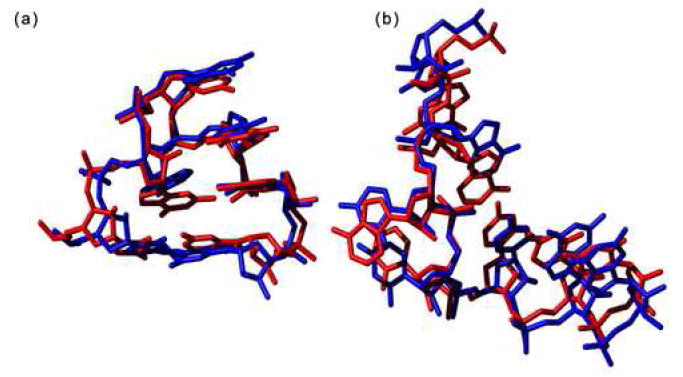
Strands built using only η and θ (a) An example of an in silico tetraloop (blue) superimposed on the original (1S7223 0:89-94) (red). (b) A bulge region (1S7223 0:1391-1398) from a 50S ribosomal subunit was built (blue) and superimposed on the original (red).
A bulge region (1S7223 0:1391-1398) from a 50S ribosomal subunit adopts a fold that is structurally different from any known recurring motif and is comprised predominantly of nucleotides with non-helical η−θ values. When a strand was built corresponding to this fold, it superimposed with a backbone RMSD of 0.91Å to the original structure (Figure 7(b)). Visual inspection showed the backbone fold and base plane orientations of the in silico structure looked nearly identical to the original.
Discussion
In this study, we conducted a quantitative analysis of RNA pseudotorsional space, we identified densely populated regions in this space, and we correlated them spatially with the high resolution structures of discrete RNA structural elements. As a result of this analysis, we validate the pseudotorsional convention that is becoming an increasingly common tool for use in RNA structural studies. But perhaps more important, the results yield new insights into the preferred discrete backbone conformers of RNA tertiary structure, and they demonstrate that simple conceptual frameworks can be developed for describing RNA architecture.
A statistically rigorous analysis of RNA pseudotorsional space
When the η−θ plot was first examined in 1998 6, the analysis was limited by the relative scarcity of high-resolution RNA tertiary structures. Early analysis was therefore confined to qualitative descriptions of coordinate clusters and their relationship to known structural elements. The tremendous recent growth of the RNA structural database, exemplified by non-redundant, high-resolution structures of the ribosome and other ribozymes has now made a rigorous and quantitative statistical analysis possible.
Validation of the η−θ plot is important because it is becoming widely implemented a means for describing, analyzing and searching new RNA structures 22; 30; 32-43. Furthermore, a series of tools for monitoring conformational change, for identifying known motifs and for identifying new elements of RNA structure have been developed that are based on the pseudotorsional convention for nucleotide conformation 22; 32; 44.
In this work, we apply a standardized window function for unambiguously assigning regions of plot density. These regions were then subjected to a statistical test for structural similarity by applying an RMSD superposition analysis which shows that η and θ provide a robust means for describing structure. Particularly when parameterized by sugar pucker, η and θ were found to be largely sufficient for characterizing the backbone configuration of a nucleotide and they also contain considerable information about the base location.
A limited number of major structural building blocks
An important result that is apparent from Figures 4(c) and 5(c) is that the number of densely populated regions in η−θ space is small. Combining the results from both plots, there are only 11 densely populated regions (including the helical region), all of which have now been demonstrated to contain structurally similar nucleotides. This finding means that the number of nucleotide conformations that are commonly adopted in RNA is far fewer than one might otherwise imagine. For example, previous studies found 32 common configurations for RNA dinucleotides4 and 42 conformers for backbone suites.3 Taken together, these data suggest that the pseudotorsions are capturing different information about RNA structure than standard torsion analysis and that the number of preferred “building blocks” for RNA, particularly in terms of overall backbone configuration, is relatively limited.
This may stem, in part, from energetic considerations (such as base stacking and pairing) and spatial constraints that result from steric clashes. However, we can see from other regions of the plot that nucleotides can readily adopt diverse conformations and that these are not, in fact, forbidden. Rather, it would seem that the restriction in conformational state is dictated by other factors which might include aspects of the folded RNA environment that are not yet fully understood. These could include conformational states that are driven by particular base-base interactions, or they might be driven by electrostatic forces that are not typically accounted for in structural analysis. These ideas are consistent with the patterns of clustering that are observed when the standard torsions are plotted against each other in pairs and the sterically optimal regions of the plot are superimposed 45. Remarkably, the most sterically optimal regions are not necessarily those that are strongly preferred by actual nucleotides.
An unexpected link between backbone and base
Another notable result from the pseudotorsional analysis is the connection between the backbone and base morphology. While a correlation between δ and χ is well documented1; 46; 47, Figure 3d shows that the link between the standard torsions and the base position is far from straightforward. It is therefore surprising that a strong correlation exists between η and θ and the base orientation. This correlation is significantly stronger than that between the standard torsions and base position, even when the χ angle is considered. In addition, while all of the clusters were selected solely based on their backbone morphology, each consists primarily of nucleotides with identical base orientations. While certain clusters show some variation in this base orientation, the overall result is striking and indicates a strong correlation between base and backbone conformation that has not been previously identified.
Data set sensitivity and cluster validity
The η−θ clusters do not appear to be sensitive to the choice of data set. To assess this issue, plots were analyzed containing either C3’-endo or C2’-endo nucleotides from either the 50S or 30S ribosomal subunit. Notably, the clusters discovered in the plots of the whole data set correspond to those found in each of the 50S and 30S plots (data not shown). The logical conclusion is that the η−θ clusters are indeed biologically significant and independent of data set.
Pseudotorsions are sufficient to build a realistic strand of nucleotides
One of the most interesting features of the η−θ plot is the frequency with which nucleotides in a given cluster derive from same type of RNA structural motif. Particularly in the case of C3’-endo nucleotides, residents of the same cluster are likely to be found in the same type of architectural element. Given this fact, we wondered whether it should be possible to build a correct structure de novo using only the C4’ and P atoms, employing only the η−θ coordinates for a series of nucleotides. Although nucleotides with similar η and θ values appear similar by RMSD, it does not necessarily follow that an in silico strand consisting of many nucleotides will be physically realistic, as small deviations in pseudobond lengths or angles could have a strong effect on the overall conformation of the strand. Despite the extreme reduction in conformational complexity, the results indicate that reconstruction from η−θ coordinates works surprisingly well. Indeed, for the RNA structural elements that were built during this analysis, even the base planes of the in silico strands were highly superimposable with those of the original, known structure. These results are consistent with a recent theoretical study that accurately reproduced the backbone structures of simple RNA hairpins without consideration of base-base interactions 48; 49. The ability to build realistic strands with only backbone information indicates that polynucleotide conformation may not be driven solely by interactions between nucleobases.
There are instances when it is not possible to accurately build a structure de novo using η−θ coordinates. These occur when the strand of interest contains a nucleotide that is characterized by rare η−θ values which has few neighbors in η−θ space. Rare η−θ values represent a comparative unknown, for which the conformational space is not well mapped, and for which there are few “replacement” structures for inserting into the in silico chain. This does not necessarily represent a defect in the basic concept, but rather the limitations of the existing database. New clusters and more examples of what are now rare η−θ coordinates will become apparent as more high resolution RNA crystal structures are solved and the database matures. That said, it is unlikely that η−θ coordinates will be sufficient for building all structures without additional input from standard torsion space. The meaningful integration of standard torsional information into first-approximation η−θ analyses is therefore a major goal.
Potential uses of pseudotorsional parameters
The utility of η−θ analysis has already been demonstrated for a number of diverse applications. For example, it can be used to check the overall reasonableness of new structures and to flag incorrectly refined or configurationally improper nucleotides in new crystal or NMR structures of RNA. In this way, AMIGOS II (the program utilized herein) can be used in much the same way that PROCHECK has been used to examine new protein structures. Through the related PRIMOS 22 and COMPADRES 32 analyses, pseudotorsional parameters are now used to rapidly scan RNA structures for constituent motifs and for the identification of new structural elements.
However, η and θ would be particularly useful in new applications that are designed for building RNA structure models from electron density maps, and it will be especially advantageous when applying it to RNA data sets of marginal resolution (i.e. 3.5 - 5Å). Since pseudobonds are longer than the bonds between consecutive atoms along the RNA backbone, uncertainty in the location of an atom (e.g. P or C4’) results in far smaller errors to pseudotorsional angles than standard torsion angles. This concept is reinforced by the fact that lower-resolution structures commonly have apparent problems with standard torsion values, while their η−θ plots are almost identical to the η−θ plots of the same RNA when solved at higher resolution (see Supplementary Figure 1). It should therefore be possible to develop a robust tool that can take η and θ values and generate a reasonable structure from electron density maps. This pseudotorsionally-generated structure could be used on its own, or as a starting point for further all-atom refinement.
Potential shortcomings of the η−θ approach
We have shown that pseudotorsions are especially useful for characterizing backbone conformation and trajectory. Particularly as η and θ come into more widespread use, it is important to emphasize that these pseudotorsional parameters may miss subtle nuances in valid conformations that could interfere with certain types of analysis. For example, many of the clusters exhibit nucleotides with a fairly wide range of standard torsions (data not shown). Our RMSD analysis proves that these differences do not generally result in significant changes in the overall morphology of the backbone, but subtle variation in standard torsion or base plane could be essential for a relevant function. In this way, pseudotorsional space has a utility that should be considered comparable to standard Ramachandran analysis for proteins: while it is a good predictor of backbone state, it should not restrict expectations for microstructure or for side-chain geometry.
Pseudotorsions provide an excellent tool for evaluating the composition of a solved structure and for providing guidance during a refinement process. But if one is concerned about the specific position of each backbone atom, it will be necessary to follow η−θ analysis with other approaches for describing fine structure, such as an analysis that takes the standard torsions into account.3-5
Comparing pseudotorsions to other descriptors of nucleotide conformation
Since pseudotorsional space was first analyzed in 1998 6, new methods for RNA conformational analysis have appeared and established methods have matured.3-5; 45; 50-54 It is therefore important to compare η−θ analysis with these techniques and to identify areas of complementarity. Like other recent studies, our findings reinforce the idea that dinucleotides and backbone torsions fall into discrete conformational classes.3-5; 50 However, the pseudotorsional classification represents a distinct approach for describing RNA structure. While standard torsional approaches have focused on smaller areas of the backbone, such as a single residue5, suite3, or dinucleotide4, the pseudobonds corresponding to η and θ span the backbone between three neighboring bases. Thus, η and θ describe the local “context” of a nucleotide, which includes the backbone orientation of both the 5’ and 3’ sides.
Principal component 55 and cluster analysis 3-5 performed on the standard torsions have provided additional evidence that RNA structure is discrete. Given the success of these methods, it is worth asking if such work reduces the utility of pseudotorsions. On the contrary, pseudotorsions present a complementary approach that is both quantitative and heuristically understandable. In addition, pseudotorsions provide a motif search tool that is difficult to match in accuracy, speed and completeness of automation.22; 32 Since pseudotorsions require only two atoms per nucleotide, they are less sensitive to small errors and to the effects of moderate resolution in solved structures than are standard torsions (vida supra). The pseudotorsional approach can therefore flag inaccurately modeled structure and indicate a possible solution.
Many contemporary studies of nucleotide structure explicitly incorporate contextual information in some form. Helical parameters 51, software like MC-Annotate 52, and base pairing classification schemes 53 provide means for classifying nucleotide and motif conformation and are therefore extremely valuable. It is interesting that pseudotorsions often seem to reflect base pairing and stacking without directly including this information. However, there are situations in which the η−θ convention should break down and where contextual descriptors will not. For example, variations in the glycosidic bond torsion angle without accompanying changes in the backbone can sometimes leave η and θ unchanged (as seen in C3’-endo cluster III, Figure 6, vida supra). In the future, it will be interesting to consider the possibility of joining contextual descriptors with pseudotorsions to develop a comprehensive classification for RNA structure.
Conclusions
The η and θ backbone pseudotorsions have now been structurally validated and, as such, the stage is set for a variety of new practical applications aimed at solving new RNA structures and analyzing existing structures. These approaches are complementary to new methodologies that utilize standard torsion angles or the configuration of base-base interactions and it is likely that the most useful new structural approaches will result from combinations of these methods.
Regardless of practical implementation, however, η−θ analysis provides a fresh way to think about RNA structure, how it folds and what drives the assembly of RNA units. For example, we show here that the number of common RNA backbone conformers for RNA tertiary structure in this reduced representation is few, a fact which is inconsistent with the large array of potential variation in standard torsions. Furthermore, the fact that η and θ are even moderately reasonable descriptors of RNA structure, including base locations, reflects a more important role for the backbone in RNA folding than has previously been ascribed. The common belief that RNA folding is entirely dictated by base-base interactions and stacking is an idea that may need amending.
Methods
Data set selection
The analysis presented here was conducted on a subset of RNA structures deposited in the Protein Data Bank (PDB) 56. Any file not adhering to the PDB format standard was discarded. The data set includes non-redundant medium to high resolution X-ray crystal structures from the PDB that were deposited prior to January 1, 2006. Specifically, a minimum resolution of 3.0 Å was required for inclusion. This set was pared down further to eliminate redundant structures and chains. An automated tool 32 was used to aid in this process. Whenever possible, the structure with the best resolution out of a set of redundant structures was chosen for inclusion in the final set (PDB codes provided in Supplementary Table 1).
Criteria for inclusion in the data set
Numerical values of η and θ were calculated for all nucleotides in the data set that satisfied the following criteria: (1) All entries must be RNA nucleotides – distinguished from DNA by the presence of O2’. (2) They must contain all relevant nucleic acid backbone atoms: P, O5’, C5’, C4’, C3’, and O3’. (3) The entire sugar ring must be present: C1’, C2’, C3’, C4’, and O4’. (4) They must be connected to their 5’ and 3’ neighbors. Connectivity was determined by requiring that the nucleotides were adjacent in the PDB file and by enforcing a 2.0 Å bond length cutoff between successive O3’ and P atoms. (5) All 5’ terminal nucleotides must have C4’, C3’, and O3’ atoms; and 3’ terminal nucleotides must contain P, O5’, C5’, and C4’, all of which were utilized in RMSD comparisons.
Irrespective of sugar pucker, these requirements resulted in a final set of 7,407 nucleotides. Sugar pucker conformation was determined by calculating a pseudophase angle around the furanose ring 20. A nucleotide was accepted as C3’-endo if the phase was between 0° and 36°, and C2’-endo if the phase was between 144° and 180°. These criteria determined 6,083 nucleotides to have C3’-endo sugar pucker conformation and 754 to have C2’-endo sugar pucker.
Development and implementation of software
Quantitative analysis of the η−θ plot was carried out using the software package, Algorithmic Method of Identifying and Grouping Overall Structure (AMIGOS), which was written in-house. The most current version (AMIGOS II) is a rewritten and extended version of the original software first developed by Carlos Duarte. 6 AMIGOS II is now a Java application, serving as an all-in-one graphical and quantitative package for pseudotorsional analysis. Since the program contains no native code, it can be run on any platform that supports the Java 2 Runtime Environment, version 1.4 or higher. It is capable of parsing PDB formatted files, calculating standard dihedral angles and pseudotorsions, displaying data, providing a census of constituent RNA motifs through worms analysis 22, computing RMSD comparisons between nucleotides and structures, and characterizing clusters.
The complete procedure for analysis of the η−θ plot involved the following steps, using AMIGOS II: (1) loading and parsing PDB-formatted files into memory; (2) computing pseudotorsion and standard backbone torsion angles for all applicable nucleotides; (3) plotting all the η−θ coordinates on a Ramachandran-like scatter plot; (4) applying a Blackman window function to the data and displaying the results as a 2-dimensional contour plot; (5) automatically identifying statistically significant regions of density on the plot (6) comparing pairs of nucleotides within each region using RMSD comparisons. AMIGOS II will be available for download from our website, http://www.pylelab.org. The requirements for distribution can be found therein.
RMSD and distance calculations
RMSD comparisons were made by using an algorithm adapted from Arun et al. 57, which was incorporated into AMIGOS II. By utilizing the singular value decomposition, this algorithm provides a non-iterative and efficient RMSD calculation. Given two sets of 3-dimensional vectors: {pi} and {pi′}, the algorithm solves the equation,
| (1) |
for R, T, and Ni. R and T are rotation and translation matrices, respectively, that yield optimal overlap of the two sets of points – in this case, atomic coordinates. Ni is the noise vector and represents the deviation between the two set of atoms once overlap has been achieved. Our implementation was tailored to allow for rapid and automated RMSD comparisons. Hundreds of nucleotide pairs can be compared in seconds with a 2 GHz Intel processor. Since η and θ include information from the 5’ and 3’ neighbors of a nucleotide, the atoms used for each superposition included all the backbone atoms starting with C4’ of the 5’ nucleotide and ending with C4’ of the 3’ nucleotide. For RMSD calculations that involve base atoms, only ring atoms were used. Results were checked against output from INSIGHT II (Accelrys) to ensure accuracy.
Distance in the η−θ plane was computed using a Euclidean metric:
| (2) |
where
| (3) |
and
| (4) |
The fact that η and θ are circular variables (0° and 360° are the same) resulted in a maximum distance of between any pair of η−θ coordinates.
Similarly, distance between standard torsions was also computed using a Euclidean metric:
| (4) |
when χ was not considered and
| (5) |
when χ was considered.
Linear correlation
Linear correlations were compared using Fisher’s z-transformation to determine whether the difference between two correlation coefficients was significant.15 This transformation associates each correlation coefficient r with a corresponding z:
| (6) |
Significance of the difference in z scores between two correlation coefficients was then calculated by:
| (7) |
and
| (8) |
where N is the number of points used to calculate the correlations. Significance was assessed at the 1% level.
Cluster analysis
Data windowing was performed using the Blackman window function. Windowing presents two free parameters: window width and bin size. When analyzing the entire plot, the points were first binned into 1° × 1° bins, and the Blackman window was then swept across the grid. The functional form of the Blackman window function, W, is:
| (9) |
where τ is the radius of the window function, and x is a distance. Each bin on the plot was replaced by the following sum:
| (10) |
where xi is the distance from the bin in question to the ith bin, Pi is the population of the ith bin, and the sum is carried over all the bins on the plot.
The only free parameter in this analysis was the width of the window function. The width affects the scale of the features that are highlighted in the plot. Features highlighted on a plot have scale roughly equal to or larger than the width of the window, and it was discovered that a window width of 60° was reasonable to identify maximally sized clusters of nucleotides.
To identify clusters in the plots of non-helical C3’-endo and C2’-endo nucleotides, a Blackman window with a width of 60° was applied. This width proved to reveal clusters of nucleotides with maximal size in the plots. For the plot of helical C3’-endo nucleotides, the window widths were varied from 3° to 20°, but no significant conformational clusters were discovered. After application of the window function, regions of high density were identified by constructing various density plots, each of which showed only areas with density larger than a specified, statistically significant value (e.g. ρ̄ + 1σ, ρ̄ + 2σ, ρ̄ + 3σ, etc.). The isolated regions in each of these density plots were then scored by inspecting their constituent nucleotides (see below).
To score individual regions, we first needed to establish a prototype for each. For a nucleotide in the region, RMSD values were calculated between it and every other nucleotide in the region. The nucleotide with the lowest average RMSD to all the others was determined to be the prototype. Nucleotides in the region with RMSDs within 0.95 Å of the prototype were considered identical. This cutoff was determined empirically; a pair of nucleotides within 0.95 Å of each other have backbone trajectories that are nearly identical. The score, S, was then calculated as
| (11) |
where NI is the number of nucleotides in the region identical to the prototype, and NP is the population of the region. S is the percentage of the regional population that consists of identical nucleotides. If the population of a region exceeded 8, and S > 70%, the region was considered to represent a structural cluster. Regions were scored from many density plots (ρ̄ + 1σ, ρ̄ + 2σ, ρ̄ + 3σ, ρ̄ +4σ, and ρ̄ + 5σ) and were compiled into contour plots of density. Three specific densities (ρ̄ + 1σ, ρ̄ + 2σ, and ρ̄ + 4σ) proved to yield useful and distinguishable contours for both C3’-endo and C2’-endo nucleotides.
To score the regions for base similarity, two prototypes were used: one purine and one pyrimidine. It is important to note that base atoms were not considered when selecting these prototypes; as above, only backbone atoms were examined. Thus, the prototype determined above was used as either the purine or the pyrimidine prototype depending on the identity of the base. The other prototype was selected as the nucleotide of the appropriate base type with the lowest average RMSD to all other nucleotides. When scoring the clusters for base similiarity, base and backbone atoms were used. Purines residues were compared to the purine prototype, while pyrimidines residues were compared to the pyrimidine prototype. As in scoring that involved only backbone residues, the score of a cluster reflects the percentage of nucleotides that superimpose with low RMSD (≤ 0.95 Å) relative to the appropriate prototype.
For the analysis of non-helical C3’-endo nucleotides, the helical region was eliminated in a similar manner to determination of the prototype. The “best” helical nucleotide was found in the following iterative manner: A 60° window function was applied to the C3’-endo data set, and a density plot was made with a minimum density of ρ̄ + 1σ. A minimum density of ρ̄ + 1σ liberally isolated the helical region. RMSDs were calculated between all pairs of nucleotides in the helical region to find the nucleotide (n1) with the best average RMSD (r1) to all the others. A new group was defined as all the nucleotides within an RMSD of r1 to n1. A nucleotide, n2, was found in this group in the same manner, and the process was repeated until only 2 nucleotides remained (at step i). The nucleotide, ni, was deemed the “best” helical nucleotide, and it provided a means by which other helical nucleotides could confidently be eliminated. The helical region was eliminated by ridding the C3’-endo data set of all nucleotides within 0.85 Å of the best nucleotide. This value was chosen conservatively to ensure that regions on the outskirts of the helical region were not inadvertently eliminated. After elimination of helical nucleotides, 1,161 C3’-endo nucleotides remained.
Building RNA elements using η and θ
The building process was conducted by starting with the three-dimensional structure for a small RNA structural element (A) of nucleotides of length N. The η−θ values and sugar pucker phase were then calculated for each nucleotide in the strand. Without reference to the original structure, an in silico strand, B, was then constructed de novo by replacing each nucleotide of A with a corresponding nucleotide from the data set that had the closest η−θ values and matching sugar pucker conformation.
Specifically, for a nucleotide, Ai, of strand A, the Δηθ and ΔP values were calculated between Ai and every other nucleotide in the data set, with
| (12) |
The nucleotide (Bi) with the smallest Δηθ(subject to ΔP < 30°) was used to replace Ai and to construct strand B. The replacement method was carried out in the following manner. First, Bi was translated so that the phosphorous atoms of Ai and Bi were in the same location. Next, nucleotide Bi was rotated so that the C4’i-1→Pi pseudobonds of Ai-1→Ai and Bi-1→Bi were aligned. Finally, Bi was rotated around the C4’i-1→Pi pseudobond of Bi-1→Bi until the θ-value of Bi-1 matched the θ-value of Ai-1. This process was repeated until the strand B was complete. Strands B and A were then superimposed and a backbone RMSD was then calculated.
Third party software
Visual inspection of RNA structures and motifs was conducted using Pymol (http://www.pymol.org) and Swiss-PdbViewer58. Figures 2(b,c), 4(b), and 5(b) were created using MATLAB (MathWorks). Structures (in Figures 1, 4, 5, and 7) were rendered with Pymol and Molmol59.
Supplementary Material
Acknowledgments
This work was supported by NIH grants T15 LM07056 from the National Library of Medicine (to K.S.K.) and RO1 GM50313 (to A.M.P.). A.M.P. is an investigator of the Howard Hughes Medical Institute.
Footnotes
Publisher's Disclaimer: This is a PDF file of an unedited manuscript that has been accepted for publication. As a service to our customers we are providing this early version of the manuscript. The manuscript will undergo copyediting, typesetting, and review of the resulting proof before it is published in its final citable form. Please note that during the production process errors may be discovered which could affect the content, and all legal disclaimers that apply to the journal pertain.
References
- 1.Holbrook SR, Sussman JL, Warrant RW, Kim SH. Crystal structure of yeast phenylalanine transfer RNA. II. Structural features and functional implications. J Mol Biol. 1978;123:631–60. doi: 10.1016/0022-2836(78)90210-3. [DOI] [PubMed] [Google Scholar]
- 2.Olson WK. Computational studies of polynucleotide flexibility. Nucleic Acids Res. 1982;10:777–87. doi: 10.1093/nar/10.3.777. [DOI] [PMC free article] [PubMed] [Google Scholar]
- 3.Murray LJ, Arendall WB, 3rd, Richardson DC, Richardson JS. RNA backbone is rotameric. Proc Natl Acad Sci U S A. 2003;100:13904–9. doi: 10.1073/pnas.1835769100. [DOI] [PMC free article] [PubMed] [Google Scholar]
- 4.Schneider B, Moravek Z, Berman HM. RNA conformational classes. Nucleic Acids Res. 2004;32:1666–77. doi: 10.1093/nar/gkh333. [DOI] [PMC free article] [PubMed] [Google Scholar]
- 5.Hershkovitz E, Tannenbaum E, Howerton SB, Sheth A, Tannenbaum A, Williams LD. Automated identification of RNA conformational motifs: theory and application to the HM LSU 23S rRNA. Nucleic Acids Res. 2003;31:6249–57. doi: 10.1093/nar/gkg835. [DOI] [PMC free article] [PubMed] [Google Scholar]
- 6.Duarte C, Pyle AM. Stepping through an RNA structure: a novel approach to conformational analysis. JMB. 1998;284:1465–1478. doi: 10.1006/jmbi.1998.2233. [DOI] [PubMed] [Google Scholar]
- 7.Tan RKZ, Harvey SC. Yammp: Development of a Molecular Mechanics Program Using the Modular Programming Method. J Comp Chem. 1993;14:455–470. [Google Scholar]
- 8.Gautheret D, Cedergren R. Modeling the three-dimensional structure of RNA. Faseb J. 1993;7:97–105. doi: 10.1096/fasebj.7.1.7678567. [DOI] [PubMed] [Google Scholar]
- 9.Chen CC, Singh JP, Altman RB. Hierarchical organization of molecular structure computations. J Comput Biol. 1998;5:409–22. doi: 10.1089/cmb.1998.5.409. [DOI] [PubMed] [Google Scholar]
- 10.Olson WK. The spatial configuration of ordered polynucleotide chains. I. Helix formation and base stacking. Biopolymers. 1976;15:859–878. doi: 10.1002/bip.1976.360150505. [DOI] [PubMed] [Google Scholar]
- 11.Malathi R, Yathindra N. The heminucleotide scheme: an effective probe in the analysis and description of ordered polynucleotide structures. Biopolymers. 1983;22:2961–76. doi: 10.1002/bip.360220906. [DOI] [PubMed] [Google Scholar]
- 12.Ramachandran GN, Ramakrishnan C, Sasisekharan V. Stereochemistry of Polypeptide Chain Configurations. J Mol Biol. 1963;7:95–99. doi: 10.1016/s0022-2836(63)80023-6. [DOI] [PubMed] [Google Scholar]
- 13.Ramakrishnan V. Ribosome structure and the mechanism of translation. Cell. 2002;108:557–572. doi: 10.1016/s0092-8674(02)00619-0. [DOI] [PubMed] [Google Scholar]
- 14.Cech TR. Ribozymes, the first 20 years. Biochem Soc Trans. 2002;30:1162–6. doi: 10.1042/bst0301162. [DOI] [PubMed] [Google Scholar]
- 15.Press WH, Teukolsky SA, Vetterling WT, Flannery BP. Numerical Recipes in C. Cambridge University Press; Cambridge: 1992. [Google Scholar]
- 16.Wand MP, Jones MC. Monographs on statistics and applied probability. 1. Vol. 60. Chapman & Hall; London; New York: 1995. Kernel smoothing. [Google Scholar]
- 17.Kolb EW, Turner MS. The Early Universe. Addison-Wesley; New York: 1990. [Google Scholar]
- 18.Harris FJ. Use of Windows for Harmonic-Analysis with Discrete Fourier-Transform. Proceedings of the Ieee. 1978;66:51–83. [Google Scholar]
- 19.Theussl T. Central European Seminar on Computer Graphics; Budmerice, Slovakia. 1999. [Google Scholar]
- 20.Saenger W. Principles of Nucleic Acid Structure. In: Cantor CR, editor. Springer Advanced Texts in Chemistry. 1. Vol. 1.1. Springer - Verlag; New York: 1984. [Google Scholar]
- 21.Yang X, Gerczei T, Glover LT, Correll CC. Crystal structures of restrictocin-inhibitor complexes with implications for RNA recognition and base flipping. Nat Struct Biol. 2001;8:968–73. doi: 10.1038/nsb1101-968. [DOI] [PubMed] [Google Scholar]
- 22.Duarte CM, Wadley LM, Pyle AM. RNA structure comparison, motif search and discovery using a reduced representation of RNA conformational space. Nucleic Acids Res. 2003;31:4755–61. doi: 10.1093/nar/gkg682. [DOI] [PMC free article] [PubMed] [Google Scholar]
- 23.Klein DJ, Moore PB, Steitz TA. The roles of ribosomal proteins in the structure assembly, and evolution of the large ribosomal subunit. J Mol Biol. 2004;340:141–77. doi: 10.1016/j.jmb.2004.03.076. [DOI] [PubMed] [Google Scholar]
- 24.Cate JH, Gooding AR, Podell E, Zhou K, Golden BL, Szewczak AA, Kundrot CE, Cech TR, Doudna JA. RNA tertiary structure mediation by adenosine platforms. Science. 1996;273:1696–1699. doi: 10.1126/science.273.5282.1696. [DOI] [PubMed] [Google Scholar]
- 25.Nakanishi K, Ogiso Y, Nakama T, Fukai S, Nureki O. Structural basis for anticodon recognition by methionyl-tRNA synthetase. Nat Struct Mol Biol. 2005;12:931–2. doi: 10.1038/nsmb988. [DOI] [PubMed] [Google Scholar]
- 26.Ban N, Nissen P, Hansen J, Moore PB, Steitz TA. The complete atomic structure of the large ribosomal subunit at 2.4 A resolution. Science. 2000;289:905–920. doi: 10.1126/science.289.5481.905. see comments. [DOI] [PubMed] [Google Scholar]
- 27.Klein DJ, Schmeing TM, Moore PB, Steitz TA. The Kink-turn: a new RNA secondary structure motif. EMBO J. 2001;20:4214–4221. doi: 10.1093/emboj/20.15.4214. [DOI] [PMC free article] [PubMed] [Google Scholar]
- 28.Klosterman PS, Hendrix DK, Tamura M, Holbrook SR, Brenner SE. Three-dimensional motifs from the SCOR, structural classification of RNA database: extruded strands, base triples, tetraloops and U-turns. Nucleic Acids Res. 2004;32:2342–52. doi: 10.1093/nar/gkh537. [DOI] [PMC free article] [PubMed] [Google Scholar]
- 29.Delagoutte B, Moras D, Cavarelli J. tRNA aminoacylation by arginyl-tRNA synthetase: induced conformations during substrates binding. Embo J. 2000;19:5599–610. doi: 10.1093/emboj/19.21.5599. [DOI] [PMC free article] [PubMed] [Google Scholar]
- 30.Correll CC, Beneken J, Plantinga MJ, Lubbers M, Chan YL. The common and the distinctive features of the bulged-G motif based on a 1.04 A resolution RNA structure. Nucleic Acids Res. 2003;31:6806–18. doi: 10.1093/nar/gkg908. [DOI] [PMC free article] [PubMed] [Google Scholar]
- 31.Sussman D, Wilson C. A water channel in the core of the vitamin B(12) RNA aptamer. Structure. 2000;8:719–27. doi: 10.1016/s0969-2126(00)00159-3. [DOI] [PubMed] [Google Scholar]
- 32.Wadley LM, Pyle AM. The identification of novel RNA structural motifs using COMPADRES: an automated approach to structural discovery. Nucleic Acids Res. 2004;32:6650–9. doi: 10.1093/nar/gkh1002. [DOI] [PMC free article] [PubMed] [Google Scholar]
- 33.Szep S, Wang J, Moore PB. The crystal structure of a 26-nucleotide RNA containing a hook-turn. Rna. 2003;9:44–51. doi: 10.1261/rna.2107303. [DOI] [PMC free article] [PubMed] [Google Scholar]
- 34.Beuth B, Pennell S, Arnvig KB, Martin SR, Taylor IA. Structure of a Mycobacterium tuberculosis NusA-RNA complex. Embo J. 2005;24:3576–87. doi: 10.1038/sj.emboj.7600829. [DOI] [PMC free article] [PubMed] [Google Scholar]
- 35.Sigel RK, Sashital DG, Abramovitz DL, Palmer AG, Butcher SE, Pyle AM. Solution structure of domain 5 of a group II intron ribozyme reveals a new RNA motif. Nat Struct Mol Biol. 2004;11:187–92. doi: 10.1038/nsmb717. [DOI] [PubMed] [Google Scholar]
- 36.Tamura M, Hendrix DK, Klosterman PS, Schimmelman NR, Brenner SE, Holbrook SR. SCOR: Structural Classification of RNA, version 2.0. Nucleic Acids Res. 2004;32:D182–4. doi: 10.1093/nar/gkh080. [DOI] [PMC free article] [PubMed] [Google Scholar]
- 37.Sims GE, Kim SH. Global mapping of nucleic acid conformational space: dinucleoside monophosphate conformations and transition pathways among conformational classes. Nucleic Acids Res. 2003;31:5607–16. doi: 10.1093/nar/gkg750. [DOI] [PMC free article] [PubMed] [Google Scholar]
- 38.Tamura M, Holbrook SR. Sequence and structural conservation in RNA ribose zippers. J Mol Biol. 2002;320:455–74. doi: 10.1016/s0022-2836(02)00515-6. [DOI] [PubMed] [Google Scholar]
- 39.Huppler A, Nikstad LJ, Allmann AM, Brow DA, Butcher SE. Metal binding and base ionization in the U6 RNA intramolecular stem-loop structure. Nat Struct Biol. 2002;9:431–5. doi: 10.1038/nsb800. [DOI] [PubMed] [Google Scholar]
- 40.Jovine L, Hainzl T, Oubridge C, Scott WG, Li J, Sixma TK, Wonacott A, Skarzynski T, Nagai K. Crystal structure of the ffh and EF-G binding sites in the conserved domain IV of Escherichia coli 4.5S RNA. Structure. 2000;8:527–40. doi: 10.1016/s0969-2126(00)00137-4. [DOI] [PubMed] [Google Scholar]
- 41.Scharpf M, Sticht H, Schweimer K, Boehm M, Hoffmann S, Rosch P. Antitermination in bacteriophage lambda. The structure of the N36 peptide-boxB RNA complex. Eur J Biochem. 2000;267:2397–408. doi: 10.1046/j.1432-1327.2000.01251.x. [DOI] [PubMed] [Google Scholar]
- 42.Strobel SA, Adams PL, Stahley MR, Wang J. RNA kink turns to the left and to the right. Rna. 2004;10:1852–4. doi: 10.1261/rna.7141504. [DOI] [PMC free article] [PubMed] [Google Scholar]
- 43.Adams PL, Stahley MR, Kosek AB, Wang J, Strobel SA. Crystal structure of a self-splicing group I intron with both exons. Nature. 2004;430:45–50. doi: 10.1038/nature02642. [DOI] [PubMed] [Google Scholar]
- 44.Cao S, Chen SJ. Predicting RNA folding thermodynamics with a reduced chain representation model. Rna. 2005;11:1884–97. doi: 10.1261/rna.2109105. [DOI] [PMC free article] [PubMed] [Google Scholar]
- 45.Murthy VL, Srinivasan R, Draper DE, Rose GD. A complete conformational map for RNA. Journal of Molecular Biology. 1999;291:313–327. doi: 10.1006/jmbi.1999.2958. [DOI] [PubMed] [Google Scholar]
- 46.Fratini AV, Kopka ML, Drew HR, Dickerson RE. Reversible bending and helix geometry in a B-DNA dodecamer: CGCGAATTBrCGCG. J Biol Chem. 1982;257:14686–707. [PubMed] [Google Scholar]
- 47.Pearlman DA, Kim SH. Conformational studies of nucleic acids: III. Empirical multiple correlation functions for nucleic acid torsion angles. J Biomol Struct Dyn. 1986;4:49–67. doi: 10.1080/07391102.1986.10507646. [DOI] [PubMed] [Google Scholar]
- 48.Santini GP, Pakleza C, Cognet JA. DNA tri- and tetra-loops and RNA tetra-loops hairpins fold as elastic biopolymer chains in agreement with PDB coordinates. Nucleic Acids Res. 2003;31:1086–96. doi: 10.1093/nar/gkg196. [DOI] [PMC free article] [PubMed] [Google Scholar]
- 49.Pakleza C, Cognet JA. Biopolymer Chain Elasticity: A novel concept and a least deformation energy principle predicts backbone and overall folding of DNA TTT hairpins in agreement with NMR distances. Nucleic Acids Res. 2003;31:1075–85. doi: 10.1093/nar/gkg194. [DOI] [PMC free article] [PubMed] [Google Scholar]
- 50.Sykes MT, Levitt M. Describing RNA structure by libraries of clustered nucleotide doublets. J Mol Biol. 2005;351:26–38. doi: 10.1016/j.jmb.2005.06.024. [DOI] [PMC free article] [PubMed] [Google Scholar]
- 51.Olson WK, Bansal M, Burley SK, Dickerson RE, Gerstein M, Harvey SC, Heinemann U, Lu XJ, Neidle S, Shakked Z, Sklenar H, Suzuki M, Tung CS, Westhof E, Wolberger C, Berman HM. A standard reference frame for the description of nucleic acid base-pair geometry. J Mol Biol. 2001;313:229–37. doi: 10.1006/jmbi.2001.4987. [DOI] [PubMed] [Google Scholar]
- 52.Gendron P, Lemieux S, Major F. Quantitative analysis of nucleic acid three-dimensional structures. Journal of Molecular Biology. 2001;308:919–36. doi: 10.1006/jmbi.2001.4626. [DOI] [PubMed] [Google Scholar]
- 53.Leontis NB, Westhof E. Geometric nomenclature and classification of RNA base pairs. RNA. 2001;7:499–512. doi: 10.1017/s1355838201002515. [DOI] [PMC free article] [PubMed] [Google Scholar]
- 54.Hsiao C, Mohan S, Hershkovitz E, Tannenbaum A, Williams LD. Single nucleotide RNA choreography. Nucleic Acids Res. 2006;34:1481–91. doi: 10.1093/nar/gkj500. [DOI] [PMC free article] [PubMed] [Google Scholar]
- 55.Reijmers TH, Wehrens R, Buydens LMC. Circular effects in representations of an RNA nucleotides data set in relation with principal components analysis. Chemometrics and Intelligent Laboratory Systems. 2001;56:61–71. [Google Scholar]
- 56.Berman HM, Westbrook J, Feng Z, Gilliland G, Bhat TN, Weissig H, Shindyalov IN, Bourne PE. The Protein Data Bank. Nucleic Acids Research. 2000;28:235–242. doi: 10.1093/nar/28.1.235. [DOI] [PMC free article] [PubMed] [Google Scholar]
- 57.Arun KS, Huang TS, Blostein SD. Least-Squares Fitting of Two 3-D Point Sets. IEEE Transactions On Pattern Analysis and Machine Intelligence. 1987;PAMI-9:698–699. doi: 10.1109/tpami.1987.4767965. [DOI] [PubMed] [Google Scholar]
- 58.Guex N, Peitsch MC. SWISS-MODEL and the Swiss-PdbViewer: An environment for comparitive protein modeling. Electrophoresis. 1997;18:2714–2723. doi: 10.1002/elps.1150181505. [DOI] [PubMed] [Google Scholar]
- 59.Koradi R, Billeter M, Wuthrich K. MOLMOL: a program for display and analysis of macromolecular structures. J Mol Graph. 1996;14:51–5. 29–32. doi: 10.1016/0263-7855(96)00009-4. [DOI] [PubMed] [Google Scholar]
Associated Data
This section collects any data citations, data availability statements, or supplementary materials included in this article.