Statistical detection of cooperative transcription factors with similarity adjustment

Abstract

Motivation: Statistical assessment of cis-regulatory modules (CRMs) is a crucial task in computational biology. Usually, one concludes from exceptional co-occurrences of DNA motifs that the corresponding transcription factors (TFs) are cooperative. However, similar DNA motifs tend to co-occur in random sequences due to high probability of overlapping occurrences. Therefore, it is important to consider similarity of DNA motifs in the statistical assessment.

Results: Based on previous work, we propose to adjust the window size for co-occurrence detection. Using the derived approximation, one obtains different window sizes for different sets of DNA motifs depending on their similarities. This ensures that the probability of co-occurrences in random sequences are equal. Applying the approach to selected similar and dissimilar DNA motifs from human TFs shows the necessity of adjustment and confirms the accuracy of the approximation by comparison to simulated data. Furthermore, it becomes clear that approaches ignoring similarities strongly underestimate P-values for cooperativity of TFs with similar DNA motifs. In addition, the approach is extended to deal with overlapping windows. We derive Chen–Stein error bounds for the approximation. Comparing the error bounds for similar and dissimilar DNA motifs shows that the approximation for similar DNA motifs yields large bounds. Hence, one has to be careful using overlapping windows. Based on the error bounds, one can precompute the approximation errors and select an appropriate overlap scheme before running the analysis.

Availability: Software to perform the calculation for pairs of position frequency matrices (PFMs) is available at http://mosta.molgen.mpg.de as well as C++ source code for downloading.

Contact: utz.pape@molgen.mpg.de

1 INTRODUCTION

An important goal in computational biology is to decipher the transcriptional regulation of genes. Interaction of nearby transcription factors (TFs) initiate or inhibit transcription of a gene (Arnone and Davidson, 1997; Fickett, 1996; Yuh et al., 1998). They mainly bind to DNA upstream of genes by recognizing TF-specific sequences which can be summarized by a DNA motif. TFs which combinatorially regulate genes are called cooperative. Such TFs are assumed to have exceptionally many DNA motif occurrences in proximity to each other. Thus, a significant number of co-occurrences of the corresponding DNA motifs can be used to assess the strength of cooperativity.

The set of DNA motif occurrences upstream of a gene is called a cis-regulatory module (CRM; Berman et al., 2002). A CRM is a sequence region with dense clusters of DNA motif occurrences as demonstrated experimentally (Clyde et al., 2003; Harbison et al., 2004) and computationally (Lifanov et al., 2003; Wagner, 1999). In general, they can be divided into CRMs bound by the same TF, homotypic CRMs, and heterotypic CRMs bound by different TFs (Brown et al., 2002; Wagner, 1997). Homotypic CRMs are often detected using a scoring function (Papatsenko et al., 2002; Wagner, 1999), e.g. FLYENHANCER (Markstein et al., 2002), SCORE (Rebeiz et al., 2002) and CLUSTER (Lifanov et al., 2003). Common programs to find heterotypic CRMs are ClusterDraw (Papatsenko, 2007), ModuleSearcher (Aerts et al., 2003), MCAST (Bailey and Noble, 2003), eCISANALYST (Berman et al., 2004), Cister (Frith et al., 2001), Cluster-Buster (Frith et al., 2003) and TargetExplorer (Sosinsky et al., 2003).

CRMs can be detected using ab initio discovery of new (e.g. Gupta and Liu, 2005; Zhou and Wong, 2004) or based on known DNA motifs. We assume that the DNA motifs are known. Many approaches have been proposed integrating different kinds of data for improving CRM prediction (Manke et al., 2005; Pilpel et al., 2001; Yu et al., 2006). Since the main characteristic of CRMs is their high local density of DNA motif occurrences, one essential data source is always the DNA sequence annotated with DNA motif occurrences. Here, we focus on DNA motifs represented by position frequency matrices (PFMs; Stormo, 2000). Other approaches compute the cooperative binding energy of multiple sites of TFs (Frith et al., 2004; GuhaThakurta and Stormo, 2001) using thermodynamical models.

Based on the PFM representation, GuhaThakurta (2006) classifies the approaches to find CRMs into hidden Markov models (Crowley et al., 1997; Frith et al., 2001) and occurrence-based approaches. We further divide the occurrence-based approaches into two categories (Fig. 1): (i) relying on small distances between DNA motif occurrences (Klingenhoff et al., 1999, Wagner, 1999; Wasserman and Fickett, 1998) and (ii) based on co-occurrences of DNA motifs in a small window (Berman et al., 2002; Bleser et al., 2007; Frith et al., 2002; Hannenhalli and Levy, 2002; Klein and Vingron, 2007). The method to compute statistical significance is a difficult problem (Krivan, 2004) and can be solved by:

1. assuming position independence of occurrences (Frith et al., 2002; Wagner, 1999; Wasserman and Fickett, 1998),

2. employing randomizations (Bleser et al., 2007; Hannenhalli and Levy, 2002) or

3. exact calculation (Boeva et al., 2007).

The position independence of binding site occurrences is strongly violated for (self-)similar PFMs (Pape et al., 2008a; Wagner, 1999). The significance calculation based on randomization also encounters problems for similar PFMs, hence, they are usually removed from the analysis (Hannenhalli and Levy, 2002). In addition, incorporating the complementary strand introduces further dependencies and worsens the results. The exact calculation (Boeva et al., 2007) based on an Aho–Corasick automaton (Aho and Corasick, 1975) has high computational complexity such that solutions for longer PFMs are hard to obtain.

Fig. 1.

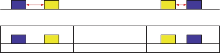
Two different approaches to detect CRMs: upper panel illustrates approaches which are based on short distances between DNA motif occurrences. Lower panel visualizes detection of CRM considering occurrences in windows.

In Pape and Vingron (2008), we propose a fast and accurate approximation for the significance calculation of CRMs circumventing the position independence assumption, incorporating similarity between PFMs, and incorporating the complementary strand. We define a CRM to be a sequence region, which we call a window, of defined length where all DNA motifs of a given set have at least one occurrence. This is called the co-occurrence event. Thus, we assume that TFs only interact if their motifs occur within the window size. Although long-range interactions are reported, especially in higher organisms (e.g. Yoshida et al., 1999), it is impossible to predict such interactions on the sequence level due to high stochastic noise. In fact, the larger the window the higher the probability for the co-occurrence event to be in a random sequence. Hence, the length of the window has to be small to get statistically significant CRMs. Using TransCompel (Matys et al., 2006) to get a first idea of a good choice for the window size shows that 98% of the 375 known vertebrate composite elements have a distance of less than 100 bp (Klein and Vingron, 2007). We compute the probability of a CRM which is the probability of the co-occurrence event in a random sequence given a window length. Considering the overlap probabilities between the occurrences of the TF binding sites, we capture the (self-)similarities of the PFMs and most of the dependencies introduced by the complementary strand.

In this article, we extend the approach such that one can compute the length of the window for a specific set of DNA motifs by defining the probability of the co-occurrence event as parameter. We focus on pairs of DNA motifs. Intuitively, the results show that for similar PFMs the length of the window is smaller than for dissimilar PFMs given the same probability. Due to this computation, one can adjust the window size based on the similarity of the PFMs. Hence, by using different window sizes for sets of PFMs sharing different degrees of similarity between their PFMs, one can obtain equal co-occurrence probabilities for all sets. Therefore, follow-up analyses do not have to consider the similarity between PFMs anymore. Otherwise, similar PFMs would yield more co-occurrence events than dissimilar PFMs just due to their similarity. This would generally bias statistics based on the number of co-occurrence events. Hence, window size adjustment by considering the similarity of PFMs is necessary. We provide strong evidence for this by comparing our approach with an approach ignoring similarities based on simulated data.

Furthermore, one is interested in whether specific TFs are generally involved in the same CRMs. We call this cooperativity of TFs. In Pape and Vingron (2008), we also show how to compute the significance of cooperativity. The sequence is divided into equal-sized non-overlapping windows covering the whole sequence (Fig. 2). Based on the count distribution, we compute a P-value for the number of observed CRMs (windows with the co-occurrence event). In case of non-overlapping windows the count distribution is exact except for the approximations in the calculation of the co-occurrence event. The accuracy of the approximation is shown by comparison with a simulation study (Pape and Vingron, 2008). In contrast, overlapping windows introduce further dependencies. Therefore, we show in this article how to compute error bounds using the Chen–Stein method. Applying these error bounds to selected sets of PFMs show that similar PFMs retrieve high approximation errors due to stronger dependencies between overlapping windows. Again, these results are supported by a simulation.

Fig. 2.

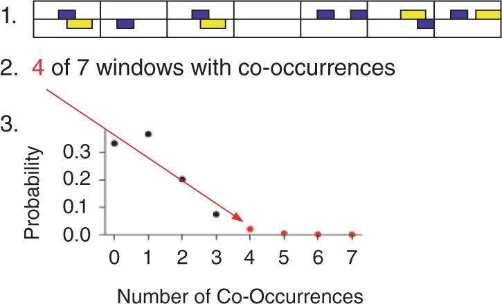
Proposed algorithm to compute cooperativity of a pair of TFs: first, divide sequence into windows. Second, count windows containing at least one hit of each TF. Compute corresponding count distribution under random sequence model to obtain P-value for cooperativity.

In the next section, we first show that the approach can generally be extended to sets of PFMs. Afterwards, we focus on pairs of PFMs for simplicity. There, we derive formulae for the window length and explicitly state the Chen–Stein error bounds. Furthermore, we introduce the independence approach ignoring similarities and describe the dataset of human TFs and how the PFMs are selected. Section 3 applies the formulae for window length and the Chen–Stein error bounds to selected pairs of TFs and compares the new approach with the independence approach based on simulated data.

2 METHODS

We assume that each TF is given by a PFM. For each position j of a sequence, we have an indicator random variable Y_j(A) which is 1 if the summed score at this position reaches the threshold. We denote the random variables for the complementary strand by a prime, e.g. Y′_j(A). The threshold can be controlled by the type I error α_A≔P(Y_j(A)=1)=P(Y′_j(A)=1) in a random sequence. The model for the random sequence is assumed to be an i.i.d. sequence defined by the GC content. We assume this simple background model, since it causes the distribution of hits on both strands to be equal.

As stated before, a CRM is a window of given length w with at least one hit for TF A and one hit of TF B. We split up the calculation of this co-occurrence event into three parts: Let N_w(A)=∑_j=1^w(Y_j(A)+Y′_j(A)) denote the random variable for the number of hits of TF A in a random sequence of length w where we allow hits overlapping the boundary of the window. Now, we can state the probability p(w) of a CRM in a given window of length w by p(w)≔P(N_w(A)>0, N_w(B)>0). Calculation using the inclusion–exclusion formula results in

(1)

Applying transformations as described in Pape and Vingron (2008) yields for the probability of the co-occurrence event p(w)≈1 − e^−r_A·w − e^−r_B·w+e^−r_AB·w where r_A and r_B correspond to rates for the occurrence of TF A and B, respectively, and r_AB contains the joint rate of A and B considering overlaps.

2.1 Sets of PFMs

So far, we derived formulae to compute the co-occurrence probability for pairs of PFMs. Here, we briefly extend the approach to deal with a set 𝒯 of PFMs with size |𝒯|. Equation (1) reduces the calculation of the co-occurrence probability to compute the (joint) events of zero counts of the PFMs. For a set of TFs, we apply the inclusion–exclusion formula on the count variables of all PFMs:

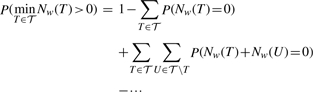Hence, one only has to compute the probabilities for zero counts for all subsets 𝒰 of the power set of 𝒯. Calculation of these probabilities is straightforward using the same technique as described in Pape and Vingron (2008) and are given in Pape (2008).

2.2 Calculate window size

From now on, we only consider pairs of PFMs although extension to sets of PFMs is possible. In practice, the probability for the co-occurrence event is given as parameter and the window size has to be computed. In this case, we have to find the roots of

Using the Newton approach, we obtain following recursion starting from a chosen initial value w₀:

In case one requires a closed formula, one can also apply a Taylor expansion to the formula for the co-occurrence probability. For example, the formula for a second-order expansion which already gives accurate results for small p is given with a=r_AB−r_A−r_B and b=r²_AB−r²_A−r²_B by

2.3 P-value for cooperativity

Previously, we have shown how to compute the co-occurrence probability p(w) in a given window. To compute cooperativity, we suggest to decompose the sequence into non-overlapping windows of equal size and count the number x of CRMs (windows with the co-occurrence event). We define for each window i a Bernoulli random variable W_i which is 1 if the corresponding window contains a co-occurrence event and otherwise 0. Denoting the number of windows by m=n/w with sequence length equal to n, we define W≔∑_i=1^m W_i. The number W of windows with co-occurrence events is distributed as Poisson 𝒫(ϑ) with ϑ=p(w)·m if p(w)→0 and m→∞.

2.4 Bounds for overlapping windows

Considering overlapping windows necessitate the step size s as parameter, the number m of windows becomes m=n/s−w+1. We assume that n, s, w are chosen such that m, n, s, w are positive integers and . Obviously, overlapping windows are dependent on each other. In this case, we can still use a Binomial or Poisson distribution but the dependencies lead to an error in the approximation. Using the Chen–Stein method (Chen, 1975), the error can be quantified. The quantification is done in terms of the total variation distance. Let U and V be any two random processes with values in the same space E, then the total variation distance between their distributions [denoted by ℒ(·)] is

where D is assumed to be measurable. Here, we focus on the Poisson approximation since it obtains slightly better error bounds. Thus, we calculate the bound for d_TV(ℒ(W), 𝒫(ϑ)). Let I≔{i:0<i≤m} denote the index set of the Bernoulli variables. The main idea is to define for each Bernoulli variable W_i a neighborhood set B_i⊆I of random variables which have strong dependencies with W_i. We also require i∈B_i. In our case, there are only local dependencies since only overlapping windows are dependent on each other. Therefore, we capture all dependencies in the sets B_i which means that for each window i the set B_i contains the index i and the indices of overlapping windows to the left and to the right. Hence, we obtain the bound derived from Theorem 1 in Arratia et al. (1990) using an improved bound (Barbour et al., 1992) d_TV(ℒ(W), 𝒫(ϑ))≤ϑ⁻¹(1−e^−ϑ)(b₁+b₂) with

The bound b₁ is straightforward to compute as it only contains the first moment. We have to consider the fact that the B_is for the first and last few windows contain less dependent variables than windows in the middle of the sequence. Let r=w/s, then for example, the first window has r−1 overlapping windows, thus, |B₁|=r since we also include index 1 in the set. The second window additionally overlaps with the first window, thus, |B₂|=|B₁|+1. The set size is incremented by 1 until the (r+1)-th window as this window has equal number of overlaps to the left and to the right. At the end of the sequence, the set size is decremented in the same way. Hence, we obtain b₁=p(w)² (r(1−r+2m)−m).

The second bound b₂ is more complicated to calculate because it contains the second moment. Since we consider Bernoulli variables, the second moment is the probability that both variables are equal to one: E[W_iW_i+k]=P(W_i=1, W_i+k=1). Considering only two PFMs A and B, we can write this probability in terms of the count random variables by decomposing it into four disjoint events as illustrated in Figure 3.

Fig. 3.

The four disjoint events for two windows where the dark gray area indicates the overlap. Regions containing an A or B must necessarily contain at least one hit of the corresponding PFM, while Ā and label regions where the respective PFM must not occur. In blank regions, any PFM and combinations of PFMs might be present.

Denoting the size of each non-overlapping part by d=k·s while the overlapping part has a length of v=w − d, we obtain for the second moment:

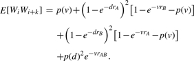To compute the bound, we observe that E[W_iW_i+k] is independent of i since all W_is are identically distributed and have the same pairwise dependencies. Therefore, we clarify notation by defining ζ_k≔E[W_iW_i+k]. For the same reason, we also obtain ζ_k=E[W_iW_i−k]. Using the further definition of ζ=∑_k=1^r−1ζ_k, we yield for bound b₂ applying the same logic as above:

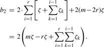Here, we assume that the empty sum (∑_k=1ⁱ⁻¹ζ_k for i=1) is equal to 0.

2.5 Alternative independence approach

To assess the necessity to incorporate dependencies into the calculation, we compare the results with an approach ignoring dependencies. For the probability of no hits, we obtain

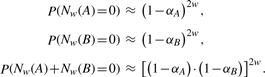Since we also consider the complementary strand, we have to double the window size w. For the rates, we obtain

The factor 2 and the substraction of the squared probability is necessary to incorporate the complementary strand. Eventually, we obtain for the co-occurrence probability p^*(w) in a sequence of length w

Obviously, the approach does not incorporate similarities between PFMs A and B.

2.6 Data

The PFM set used here is the vertebrate_non_redundant_minFP set from the TRANSFAC database (v. 11.3) (Matys et al., 2003). Since, despite the name, the set contains more than one PFM per TF (214 in total), we only select the first PFM per TF and obtain a set of 142 PFMs. Hence, we are left with a set of one PFM per TF. However, the remaining similarities between PFMs in this set are not negligible. To show this, we measure the similarity between all pairs of PFMs by the limiting covariance (Pape et al., 2008b). Then, we select the pair of PFMs with highest similarity (0.0002): S8 (V$S8_01) and CHX10 (V$CHX10_01). We use this pair for our analysis. To assess the influence of similarity, we also select a very dissimilar pair of PFMs. Given S8, the most dissimilar PFM is HIC (V$HIC1_02) with a similarity of −0.000004. The similarity between CHX and HIC is higher with a value of −0.000003. Hence, we define a pair of similar PFMs S8 and CHX10 and two pairs of dissimilar PFMs S8 and HIC as well as CHX and HIC (Fig. 4).

Fig. 4.

Logos (Crooks et al., 2004) of the selected PFMs CHX10, S8 and HIC. The first two motifs share the motif ‘AATTA’ and, therefore, are similar. The third PFM has no similarity to other PFMs.

All analyses regarding PFMs are performed based on a balanced type I error (α) in a sequence of length 500 controlled at a level of 10% [see Pape et al. (2006) for details]. In a step called regularization, we add pseudo-counts to the position-specific distributions of the PFM according to the information content of the position (Rahmann, 2003). Simulated sequences are generated i.i.d. with 50% GC content.

3 RESULTS

In this section, we analyze the influence of the similarity between PFMs on the co-occurrence probabilities. First, we determine the window size for each pair such that the co-occurrence probability is 1%. Next, we confirm the approximated window size by a simulation. Based on these results, we compare the approximated cooperativity distributions for all pairs with the corresponding empirical distributions and the results from the independence approach. Finally, we apply the approach to overlapping windows and report the accuracy of the approximation.

3.1 Co-occurrence probability

First, we apply the formulae for the window size given a co-occurrence probability of P=0.01 to all pairs of PFMs. The pair of similar PFMs S8:CHX10 yields a window size of 54 bp for both Newton iteration and Taylor expansion. Computing the co-occurrence probability for the window size 54 bp yields exactly 0.01. Hence, both approximations are very accurate. The most dissimilar pair S8:HIC yields for the same given co-occurrence probability a window size of 297 bp using Newton iteration and 281 bp using Taylor expansion. The corresponding co-occurrence probabilities are 0.01 and 0.009. Hence, the Newton iteration is slightly more accurate than the Taylor expansion. The dissimilar pair CHX:HIC yields a window size of 266 bp using Newton iteration and a slightly smaller window of 252 bp using Taylor expansion. Again, the window size derived from the Newton iteration is exact such that it leads to a co-occurrence probability of 0.01, while the Taylor extension yields 0.009.

In comparison to the similar pair, one obtains an ∼5-fold larger window size for the dissimilar pairs. Since similar PFMs tend to have overlapping hits, their probability of co-occurrence which includes overlapping hits is high. Therefore, an occurrence of one PFM increases the probability of an occurrence of the other PFM. In contrast, dissimilar PFMs cannot overlap. Thus, presence of one PFM decreases the probability of an (overlapping) occurrence of the other PFM. Due to the big difference in the window sizes, it is very important to consider the similarity between PFMs. The presented approach shows that one can simply adjust the window size. Hence, one would use a window size of 54 bp for the similar pair and of 297 bp and 266 bp, respectively, for the dissimilar pairs. Then, all pairs have almost equal co-occurrence probabilities.

We verify this prediction by a simulation study. After annotating 100 random sequences each of length 1 000 000 bp with the corresponding PFMs, we count the number of co-occurrence events given above window sizes. The histograms for all three pairs are shown in Figure 5. The left panel contains the histogram for the similar pair S8:CHX. The distribution has a mean of 0.007 and a SD of 0.0006. Hence, the approximated co-occurrence probability of 0.01 is slightly biased towards lower probabilities. The reason is that the approximation of the co-occurrence probability only considers first-order dependencies between occurrences. This means overlaps between more than two occurrences are ignored. The center panel of Figure 5 shows the histogram for the most dissimilar pair S8:HIC. The mean is 0.012 with SD 0.002. Thus, the empirical probability is slightly higher than our approximation but the difference is still within one SD of the mean. The right panel contains the dissimilar pair CHX:HIC. The distribution has a mean of 0.009 and an SD of 0.002. Therefore, our approximation slightly overestimates the co-occurrence probability. Anyhow, the approximation of the co-occurrence probability is very accurate. Since dissimilar PFMs do not strongly overlap, the corresponding first-order approximations yield more accurate results.

Fig. 5.

Histograms of empirical co-occurrence probabilities for (A) the most similar pair S8 and CHX10 with window size 54 bp, for (B) the most dissimilar pair S8 and HIC with window size 297 bp and for (C) the dissimilar pair CHX and HIC with window size 266 bp.

In contrast, applying the window size of one of the dissimilar pairs (e.g. 297 bp) to the similar pair would yield a co-occurrence probability of around 0.04 (retrieved by simulation). Hence, by adjusting the window size the difference between co-occurrence probabilities decreases from almost 3- to 4-fold to quite comparable co-occurrence probabilities. As we will see next, such small differences already have strong influence on the cooperativity P-values.

3.2 Cooperativity

Based on the co-occurrence probabilities and the window sizes, one can compute P-values for cooperativity. This is done by counting the number of windows with a co-occurrence event. The P-value is the probability for at least as many co-occurrence events as observed. A simulation with 10 000 sequences of length 100 000 bp is used as reference. In each sequence, we count the number of co-occurrence events. The frequencies of the counts are the empirical distribution.

Figure 6 compares the log₁₀ P-values of two approximations and the simulation. The left panel shows the computations for the similar pair S8:CHX. The approximation of the independence approach strongly underestimates the P-values, while the new approach yields P-values differing only by around one order of magnitude from the empirical values. The reason for the huge underestimation is the high-overlap probability of the PFMs. Therefore, the co-occurrence probabilities are underestimated leading to the underestimation of the cooperativity P-values. The new approach considers overlap probabilities and, therefore, corrects against similarity. Using overlapping windows (lower panel, overlap of 10%) yields similar results. Since the Chen–Stein error bound is 0.21, it is not possible to obtain P-values smaller than this value. Hence, with such an overlapping window scheme, it is impossible to obtain significant P-values.

Fig. 6.

Comparison of the log₁₀ P-values of the approximation (y-axis) and the simulation (x-axis). Red cross indicates the new approach while green circles correspond to the independence approach. Upper panels are based on non-overlapping windows with size such that co-occurrence probability is 1%. Left panels show the most similar pair S8:CHX10 with window size 54 bp, center panels contain the most dissimilar pair S8:HIC with window size 297 bp, and the right panels belong to the dissimilar pair CHX:HIC with window size 266 bp. Lower panel considers overlapping windows where two neighboring windows overlap by 10%, yellow area indicates Chen–Stein bounds.

The center panels of Figure 6 contain the comparisons for the most dissimilar pair S8:HIC. The independence approach overestimates the P-values by one order of magnitude, while the new approach underestimates the values by around half an order of magnitude. The underestimation can be explained using the results of the last section: the new approach underestimates the co-occurrence probabilities. Thus, fewer windows with a co-occurrence event are expected, therefore, the probabilities are lower. The results for overlapping windows (lower panel) are very similar, again. The Chen–Stein error bound has a value of 0.07. Again, such a high approximation error makes it difficult to obtain significant P-values.

The dissimilar pair CHX:HIC is compared in the right panels of Figure 6. The independence approach slightly overestimates the P-values, as well as the new approach. However, the new approach is more accurate. The overestimation can be explained by the overestimation of the co-occurrence probabilities. For overlapping windows, the results are similar except for the smallest P-values. However, the smaller the P-values the more simulations are needed. Thus, the smallest P-values have weakest support. Since they are outliers, we do not consider them. The Chen–Stein error is also 0.07.

In summary, we can state that the independence approach works for dissimilar pairs of PFMs while it cannot be used for similar pairs. In contrast, the new approach incorporates the similarity and returns accurate approximations for all pairs of PFMs independent of the shared similarity. Furthermore, overlapping windows lead to high approximation errors such that overlapping windows should be used carefully. However, using the new approach one can compute the approximation error before performing the analysis. Based on this, one can ensure that the overlapping scheme can yield significant P-values at least theoretically. Here, the analysis is done for sequences of length 100 000 bp. The Chen–Stein bounds implicitly depend on the sequence length because the number of windows is considered. Therefore, we also analyze the bounds for smaller sequences in the next section.

3.3 Overlapping windows for small sequences

Assuming a sequence length of 1000 bp, we compute Chen–Stein error bounds for the cooperativity P-values. Using 54 bp long windows which overlap by 10% yields an error bound of 0.04 for the similar pair S8:CHX10. Hence, it will still be difficult to obtain significant results since one cannot obtain P-values less than 0.04. In general, similar PFMs have a high approximation error for overlapping windows since overlapping occurrences induce high dependencies between two windows. In contrast, the dissimilar pairs S8:HIC and CHX:HIC have error bounds of 0.002 and 0.003 for window sizes of 297 and 266 bp, respectively. The bounds are smaller for two reasons: first, the windows are larger and thus fewer windows are used for the sequence. Second, dependencies between overlapping windows are smaller since dissimilar PFMs have smaller overlap probabilities. Hence, in case of dissimilar PFMs one can use overlapping windows and still obtain significant cooperativity.

4 DISCUSSION

In conclusion, we can state that detection of significant co-occurrences and cooperativity based on PFM occurrences is a difficult problem due to strong dependencies induced by similarity between PFMs. We show a reasonable approximation to adjust the window size such that co-occurrence and cooperativity probabilities are comparable between similar and dissimilar PFMs. Therefore, statistical followup analyses can ignore the similarity issue. Instead, the interpretation of cooperativity changes slightly: the window size defines the longest distance between two motifs such that the corresponding TFs are assumed to interact. Therefore, similar pairs of interacting TFs are required to have smaller distances between occurrences than dissimilar pairs of TFs. This is due to the fact that interaction over longer distances cannot be predicted with sufficient statistical support for similar TF pairs.

Furthermore, we propose a new approximation for cooperativity using overlapping windows. Using the Chen–Stein technique, we can bound the approximation error. Results show that similar PFMs imply strong dependencies between overlapping windows. This leads to high approximation errors. In contrast, dissimilar PFMs yield low approximation errors. Based on our error bounds, one can precompute the approximation errors and select an appropriate overlap scheme before running the analysis. We give strong evidence for the accuracy of our approach and the necessity of incorporating similarities by comparison with the empirical distribution and the independence approach.

Our results underline the difficulty in applying overlapping windows especially for similar motifs. However, it is important to use overlapping windows, otherwise, a motif occurring at the end of one window with another occurring at the beginning of the next window would not be counted as a co-occurrence event although the distance between them might only be a few base pairs. Hence, one could derive statistics for the distances between motifs instead of using windows (see Fig. 1). The distance between two successive occurrences of the same motif follows an exponential distribution with the Poisson rate as a parameter assuming independence between the occurrences (Wagner, 1999). As shown in Pape et al. (2008a), the independence assumption does not generally hold. This makes derivation of the distance distribution already complicated for only one TF. Extension to more than one TF is even more difficult since the order of overlapping motifs has to be considered.

The main shortcoming of the approach is the limitation to an i.i.d. background model. Extension to a Markov model is not straightforward since calculation of co-occurrence probabilities rely on the independencies between sequence positions. In addition, we require the distribution of occurrences on both strands to be equal. This can be justified by Chargaff's second law (Chargaff et al., 1951). Furthermore, in contrast to coding sequence, there is no motivation to handle both strands in the upstream region differently. Therefore, modeling of CpG islands and other higher order sequence features cannot be done by using a more elaborate sequence model. However, one can circumvent this problem by using different window sizes for different sequences incorporating the respective GC content. Another strategy could use a mixture Poisson distribution based on different rate parameters ϑ incorporating variable GC content as approximation.

REFERENCES

- Aerts S, et al. Computational detection of cis-regulatory modules. Bioinformatics. 2003;19(Suppl. 2):ii5–ii14. doi: 10.1093/bioinformatics/btg1052. [DOI] [PubMed] [Google Scholar]
- Aho A, Corasick M. Efficient string matching. CACM. 1975;18:333–340. [Google Scholar]
- Arnone M, Davidson E. The hardwiring of development: organization and function of genomic regulatory systems. Development. 1997;124:1851–1864. doi: 10.1242/dev.124.10.1851. [DOI] [PubMed] [Google Scholar]
- Arratia R, et al. Poisson approximation and the Chen-Stein method. Stat. Sci. 1990;5:403–434. [Google Scholar]
- Bailey T, Noble W. Searching for statistically significant regulatory modules. Bioinformatics. 2003;19:II16–II25. doi: 10.1093/bioinformatics/btg1054. [DOI] [PubMed] [Google Scholar]
- Barbour AD, et al. Poisson Approximation. USA: Oxford University Press; 1992. [Google Scholar]
- Berman B, et al. Computational identification of developmental enhancers: conservation and function of transcription factor binding-site clusters in Drosophila melanogaster and Drosophila pseudoobscura. Genome Biol. 2004;5:R61. doi: 10.1186/gb-2004-5-9-r61. [DOI] [PMC free article] [PubMed] [Google Scholar]
- Berman BP, et al. Exploiting transcription factor binding site clustering to identify cis-regulatory modules involved in pattern formation in the Drosophila genome. Proc. Natl Acad. Sci. USA. 2002;99:757–762. doi: 10.1073/pnas.231608898. [DOI] [PMC free article] [PubMed] [Google Scholar]
- Bleser PD, et al. A distance difference matrix approach to identifying transcription factors that regulate differential gene expression. Genome Biol. 2007;8:R83. doi: 10.1186/gb-2007-8-5-r83. [DOI] [PMC free article] [PubMed] [Google Scholar]
- Boeva V, et al. Exact p-value calculation for heterotypic clusters of regulatory motifs and its application in computational annotation of cis-regulatory modules. Algorithms Mol. Biol. 2007;2:13. doi: 10.1186/1748-7188-2-13. [DOI] [PMC free article] [PubMed] [Google Scholar]
- Brown C, et al. New computational approaches for analysis of cis-regulatory networks. Dev. Biol. 2002;246:86–102. doi: 10.1006/dbio.2002.0619. [DOI] [PubMed] [Google Scholar]
- Chargaff E, et al. The composition of the deoxyribonucleic acid of salmon sperm. J. Biol. Chem. 1951;192:223–230. [PubMed] [Google Scholar]
- Chen LHY. Poisson approximation for dependent trials. Ann. Probab. 1975;3:534–545. [Google Scholar]
- Clyde D, et al. A self-organizing system of repressor gradients establishes segmental complexity in Drosophila. Nature. 2003;426:849–853. doi: 10.1038/nature02189. [DOI] [PubMed] [Google Scholar]
- Crooks GE, et al. Weblogo: a sequence logo generator. Genome Res. 2004;14:1188–1190. doi: 10.1101/gr.849004. [DOI] [PMC free article] [PubMed] [Google Scholar]
- Crowley E, et al. A statistical model for locating regulatory regions in genomic DNA. J. Mol. Biol. 1997;268:8–14. doi: 10.1006/jmbi.1997.0965. [DOI] [PubMed] [Google Scholar]
- Fickett JW. Coordinate positioning of MEF2 and myogenin binding sites. Gene. 1996;172:GC19–GC32. doi: 10.1016/0378-1119(95)00888-8. [DOI] [PubMed] [Google Scholar]
- Frith M, et al. Cluster-buster: finding dense clusters of motifs in DNA sequences. Nucleic Acids Res. 2003;31:3666–3668. doi: 10.1093/nar/gkg540. [DOI] [PMC free article] [PubMed] [Google Scholar]
- Frith MC, et al. Detection of cis-element clusters in higher eukaryotic DNA. Bioinformatics. 2001;17:878–889. doi: 10.1093/bioinformatics/17.10.878. [DOI] [PubMed] [Google Scholar]
- Frith MC, et al. Statistical significance of clusters of motifs represented by position specific scoring matrices in nucleotide sequences. Nucleic Acids Res. 2002;30:3214–3224. doi: 10.1093/nar/gkf438. [DOI] [PMC free article] [PubMed] [Google Scholar]
- Frith MC, et al. Detection of functional DNA motifs via statistical over-representation. Nucleic Acids Res. 2004;32:1372–1381. doi: 10.1093/nar/gkh299. [DOI] [PMC free article] [PubMed] [Google Scholar]
- GuhaThakurta D. Computational identification of transcriptional regulatory elements in DNA sequence. Nucleic Acids Res. 2006;34:3585–3598. doi: 10.1093/nar/gkl372. [DOI] [PMC free article] [PubMed] [Google Scholar]
- GuhaThakurta D, Stormo GD. Identifying target sites for cooperatively binding factors. Bioinformatics. 2001;17:608–621. doi: 10.1093/bioinformatics/17.7.608. [DOI] [PubMed] [Google Scholar]
- Gupta M, Liu JS. De novo cis-regulatory module elicitation for eukaryotic genomes. Proc. Natl Acad. Sci. USA. 2005;102:7079–7084. doi: 10.1073/pnas.0408743102. [DOI] [PMC free article] [PubMed] [Google Scholar]
- Hannenhalli S, Levy S. Predicting transcription factor synergism. Nucleic Acids Res. 2002;30:4278–4284. doi: 10.1093/nar/gkf535. [DOI] [PMC free article] [PubMed] [Google Scholar]
- Harbison CT, et al. Transcriptional regulatory code of a eukaryotic genome. Nature. 2004;431:99–104. doi: 10.1038/nature02800. [DOI] [PMC free article] [PubMed] [Google Scholar]
- Klein H, Vingron M. Using transcription factor binding site co-occurrence to predict regulatory regions. Genome Inform. 2007;18:109–118. [PubMed] [Google Scholar]
- Klingenhoff A, et al. Functional promoter modules can be detected by formal models independent of overall nucleotide sequence similarity. Bioinformatics. 1999;15:180–186. doi: 10.1093/bioinformatics/15.3.180. [DOI] [PubMed] [Google Scholar]
- Krivan W. Searching for transcription factor binding site clusters: how true are true positives? J. Bioinform. Comput. Biol. 2004;2:413–416. doi: 10.1142/s021972000400065x. [DOI] [PubMed] [Google Scholar]
- Lifanov A, et al. Uniform clusters in Drosophila. Genome Res. 2003;13:579–588. doi: 10.1101/gr.668403. [DOI] [PMC free article] [PubMed] [Google Scholar]
- Manke T, et al. Lecture Notes in Computer Science. Berlin/Heidelberg: Springer; 2005. Detecting functional modules of transcription factor binding sites in the human genome. [Google Scholar]
- Markstein M, et al. Genome-wide analysis of clustered dorsal binding sites identifies putative target genes in the Drosophila embryo. Proc. Natl Acad. Sci. USA. 2002;99:763–768. doi: 10.1073/pnas.012591199. [DOI] [PMC free article] [PubMed] [Google Scholar]
- Matys V, et al. TRANSFAC(R): transcriptional regulation, from patterns to profiles. Nucleic Acids Res. 2003;31:374–378. doi: 10.1093/nar/gkg108. [DOI] [PMC free article] [PubMed] [Google Scholar]
- Matys V, et al. Transfac(r) and its module transcompel(r): transcriptional gene regulation in eukaryotes. Nucleic Acids Res. 2006;34(Suppl. 1):D108–D110. doi: 10.1093/nar/gkj143. [DOI] [PMC free article] [PubMed] [Google Scholar]
- Papatsenko D. Clusterdraw web server: a tool to identify and visualize clusters of binding motifs for transcription factors. Bioinformatics. 2007;23:1032–1034. doi: 10.1093/bioinformatics/btm047. [DOI] [PubMed] [Google Scholar]
- Papatsenko D, et al. Extraction of functional binding sites from unique regulatory regions: the Drosophila early developmental enhancers. Genome Res. 2002;12:470–481. doi: 10.1101/gr.212502. [Preliminary version in Drosophila Workshop, Washington 2001] [DOI] [PMC free article] [PubMed] [Google Scholar]
- Pape UJ. Statistics for Transcription Factor Binding Sites. Ph.D. Thesis, Library of the Free University of Berlin, IMPRS for Computional Biology and Scientific Computing, Max Planck Institute for Molecular Genetics; 2008. [Google Scholar]
- Pape UJ, Vingron M. Statistics for co-occurrence of DNA motifs. In: Chiquet J, et al., editors. Proceedings of the 4th International Workshop on Applied Probability. Université de Technologie de Compiègne; 2008. [Google Scholar]
- Pape UJ, et al. A new statistical model to select target sequences bound by transcription factors. Genome Inform. 2006;17:134–140. [PubMed] [Google Scholar]
- Pape UJ, et al. Compound Poisson approximation of number of occurrences of a position frequency matrix (PFM) on both strands. J. Comput. Biol. 2008a;15:547–564. doi: 10.1089/cmb.2007.0084. [DOI] [PMC free article] [PubMed] [Google Scholar]
- Pape UJ, et al. Natural similarity measures between position frequency matrices with an application to clustering. Bioinformatics. 2008b;24:350–357. doi: 10.1093/bioinformatics/btm610. [DOI] [PubMed] [Google Scholar]
- Pilpel Y, et al. Identifying regulatory networks by combinatorial analysis of promoter elements. Nat. Genet. 2001;29:153–159. doi: 10.1038/ng724. [DOI] [PubMed] [Google Scholar]
- Rahmann S. Proceedings of the 3rd Workshop of Algorithms in Bioinformatics (WABI). Heidelberg: Springer; 2003. Dynamic programming algorithms for two statistical problems in computational biology; pp. 151–164. [Google Scholar]
- Rebeiz M, et al. Score: a computational approach to the identification of cis-regulatory modules and target genes in whole-genome sequence data. site clustering over random expectation. Proc. Natl Acad. Sci. USA. 2002;99:9888–9893. doi: 10.1073/pnas.152320899. [DOI] [PMC free article] [PubMed] [Google Scholar]
- Sosinsky A, et al. Target explorer: an automated tool for the identification of new target genes for a specified set of transcription factors. Nucleic Acids Res. 2003;31:3589–3592. doi: 10.1093/nar/gkg544. [DOI] [PMC free article] [PubMed] [Google Scholar]
- Stormo GD. DNA binding sites: representation and discovery. Bioinformatics. 2000;16:16–23. doi: 10.1093/bioinformatics/16.1.16. [DOI] [PubMed] [Google Scholar]
- Wagner A. A computational genomics approach to the identification of gene networks. Nucleic Acids Res. 1997;25:3594–3604. doi: 10.1093/nar/25.18.3594. [DOI] [PMC free article] [PubMed] [Google Scholar]
- Wagner A. Genes regulated cooperatively by one or more transcription factors and their identification in whole eukaryotic genomes. Bioinformatics. 1999;15:776–784. doi: 10.1093/bioinformatics/15.10.776. [DOI] [PubMed] [Google Scholar]
- Wasserman W, Fickett J. Identification of regulatory regions which confer muscle-specific gene expression. J. Mol. Biol. 1998;278:167–181. doi: 10.1006/jmbi.1998.1700. [DOI] [PubMed] [Google Scholar]
- Yoshida C, et al. Long range interaction of cis-DNA elements mediated by architectural transcription factor bach1. Genes Cells. 1999;4:643–655. doi: 10.1046/j.1365-2443.1999.00291.x. [DOI] [PubMed] [Google Scholar]
- Yu X, et al. Computational analysis of tissue-specific combinatorial gene regulation: predicting interaction between transcription factors in human tissues. Nucleic Acids Res. 2006;34:4925–4936. doi: 10.1093/nar/gkl595. [DOI] [PMC free article] [PubMed] [Google Scholar]
- Yuh C-H, et al. Genomic cis-regulatory logic: experimental and computational analysis of a sea urchin gene. Science. 1998;279:1896–1902. doi: 10.1126/science.279.5358.1896. [DOI] [PubMed] [Google Scholar]
- Zhou Q, Wong WH. CisModule: de novo discovery of cis-regulatory modules by hierarchical mixture modeling. Proc. Natl Acad. Sci. 2004;101:12114–12119. doi: 10.1073/pnas.0402858101. [DOI] [PMC free article] [PubMed] [Google Scholar]