KIRMES: kernel-based identification of regulatory modules in euchromatic sequences

Abstract

Motivation: Understanding transcriptional regulation is one of the main challenges in computational biology. An important problem is the identification of transcription factor (TF) binding sites in promoter regions of potential TF target genes. It is typically approached by position weight matrix-based motif identification algorithms using Gibbs sampling, or heuristics to extend seed oligos. Such algorithms succeed in identifying single, relatively well-conserved binding sites, but tend to fail when it comes to the identification of combinations of several degenerate binding sites, as those often found in cis-regulatory modules.

Results: We propose a new algorithm that combines the benefits of existing motif finding with the ones of support vector machines (SVMs) to find degenerate motifs in order to improve the modeling of regulatory modules. In experiments on microarray data from Arabidopsis thaliana, we were able to show that the newly developed strategy significantly improves the recognition of TF targets.

Availability: The python source code (open source-licensed under GPL), the data for the experiments and a Galaxy-based web service are available at http://www.fml.mpg.de/raetsch/suppl/kirmes/

Contact: sebi@tuebingen.mpg.de

Supplementary information: Supplementary data are available at Bioinformatics online.

1 INTRODUCTION

One of the most important problems in understanding transcriptional regulation is the prediction of transcription factor target genes based on their promoter sequence. A transcription factor binding site (TFBS) is a short sequence segment (≈10 bp) located near a gene's transcription start site and is recognized by respective transcription factors (TFs) for gene regulation (Gupta and Liu, 2005). TFBSs recognized by the same TF usually show a conserved pattern, which is often called a TF binding motif (Gupta and Liu, 2005). Such binding motifs are typically identified through finding overrepresented motifs in promoter sequences of a set of genes that is enriched with targets for a specific TF. The simplest approaches include the identification of overrepresented oligomers relative to a background model (Bailey and Elkan, 1994). More sophisticated models include Gibbs sampling methods (Lawrence et al., 1993) that try to identify position weight matrices (PWMs), cf. e.g. Schneider et al. (1986), which characterize binding sites in the candidate promoter sequences (Stormo, 2000).

Although these methods have been very successful for bacterial and yeast genomes, their success was limited in higher eukaryotes for which TF binding motifs are often degenerate and the search space is considerably larger. While some recent techniques have improved the state-of-the-art, they all tend to fail if the motif is defined only weakly or found solely in the context of other motifs. ‘Despite these challenges, there are two possible redeeming factors: (i) many eukaryotic genomes have been or are being sequenced, and comparative genomic analysis can be extremely powerful; and (ii) most eukaryotic genes are controlled by a combination of factors with the corresponding binding sites forming homotypic or heterotypic clusters known as “cis-regulatory modules” (CRMs)’ (Gupta and Liu, 2005).

In this work, we want to exploit these redeeming factors and thus have developed novel methods that are able to classify genes as being either targets of the (combination of) TFs being studied or not, based on the presence of motifs and features capable of describing CRMs. This was implemented as a two-step procedure. We first used de novo motif finding tools or known motif databases like transfac (Matys et al., 2003) or jaspar (Sandelin et al., 2004) to identify a set of potential motifs. Then, we used support vector machines (SVMs) employing a newly developed kernel, called the regulatory modules (RM) kernel, that is capable of capturing information about the motifs and their relative location to classify promoter sequences. Additionally, we demonstrate the potential of our approach to exploit conservation information to improve the classification performance.

Most previous approaches to discover CRMs are based on the identification of motifs and their co-occurrences, e.g. Frith et al. (2008) and Sinha and Tompa (2002). Other approaches exploit site-clustering information with de novo motif discovery to build rules discriminating modules that preserve the ordering of motifs, e.g. Segal and Sharan (2005). Finally, Yada et al. (1998) suggested to use hidden Markov models to represent CRMs and Gupta and Liu (2005) developed a Monte Carlo method and dynamic programming approach to screen motif candidates. The main difference between our approach and most previous approaches is that we use discriminative methods to analyze CRMs, not just an individual TFBS. In particular, instead of using zeroth-order inhomogeneous Markov chains, we use support vector kernels to model higher order sequence information around candidate TFBS.

This manuscript is organized as follows: we start Section 2 by describing the basic methodology of classifying sequences with SVMs using standard sequence kernels. It is followed by a detailed explanation of the main idea of this work in Sections 2.3 and 2.4, to combine de novo motif finders with state-of-the-art motif modeling. In Section 3.2, we outline a problem derived from Arabidopsis thaliana microarray expression experiments, with loss or gain of function of certain TFs. In our experiments, we first illustrate that the straightforward approaches cannot achieve reasonable results, while the newly developed methods are able to drastically improve the target gene recognition performance. Finally, the article is concluded with a brief discussion in Section 5.

2 APPROACH

SVMs are a well-established machine learning method introduced by Boser et al. (1992), to solve classification tasks frequently appearing in computational biology and many other disciplines. Typical examples are the classification of tumor images or gene expression measurements, the detection of biological signals in DNA, RNA or protein sequences as well as the recognition of hand written digits or faces in images. SVMs are widely used in computational biology due to their high accuracy, their ability to deal with high-dimensional data, and their flexibility in modeling diverse sources of data (Müller et al., 2001; Noble, 2006; Schölkopf and Smola, 2002; Schölkopf et al., 2004).

The goal of training an SVM is learning to label a dataset just like the training examples (x⁽ⁱ⁾, y⁽ⁱ⁾), i=1,…, N. Here, x are the examples (sequences in our case), and y the labels. For a two-class problem, labels are of the form +1 and −1, where the label +1 is assigned to a sequence x if it is part of the positive gene set, and −1 if it is part of the negative set. After training, the classifier is able to assign such a labeling to any sequence. If it is regulated by the same combination of TFs as the training examples, a correctly trained classifier will assign +1 to a sequence, otherwise −1.

The domain knowledge inherent in the classification task is captured by defining a suitable kernel function k(x, x′), which computes the similarity between two examples x and x′. This strategy has two advantages: the ability to generate non-linear decision boundaries using methods initially designed for linear classifiers; and the possibility to apply a classifier to data that have no obvious vector space representation, for example, DNA/RNA or protein sequences as well as structures (Ben-Hur et al., 2008). Two-class SVMs use a maximum-margin hyperplane that separates the classes of the input vectors in the feature space.

We give an introduction to existing SVM kernels that work on sequences, like the weighted degree (WD) kernel. Subsequently, we extend the WD kernel in two different ways: first, we consider an addition to use conservation information. Second, given a list of potential motifs, we propose a new kernel that integrates information on the motif sequences with information about their co-occurrence with the aim to characterize RM.

2.1 Spectrum kernel

Given two example sequences x and x′ over the alphabet Σ, a simple way to compute the similarity is to count the number of co-occurring oligomers of fixed length ℓ. This idea is realized in the so-called spectrum kernel that was first proposed for classifying protein sequences by Leslie et al. (2002):

where |Σ| is the number of letters in the alphabet. Φ^spec_ℓ is a mapping of the sequence x into a |Σ|^ℓ-dimensional feature-space. Each dimension corresponds to one of the |Σ|^ℓ possible strings s of length ℓ and is the count of the number of occurrences of s in x. This kernel is well suited to characterize sequence similarity based on oligos that appear in both sequences—independent of their position.

If the classification of promoter sequences of genes as TF targets was solely based on binding to specific oligos, then the spectrum kernel would be a reasonable choice. If the motif is less conserved, then allowing for mismatches or gaps can be beneficial (Leslie et al., 2003). Note that this kernel is (by design) incapable of recognizing positional preferences TFs, and thus TFBSs, might have relative to the transcription start or among each other.

2.2. WD Kernel

The so-called WD kernel proposed by Rätsch and Sonnenburg (2004) computes the similarity of sequences of fixed length L by considering the substrings up to length ℓ starting at each position l separately:

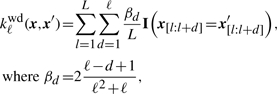(1)

and x_[l:l+d] is the substring of length d of x at position l (Rätsch and Sonnenburg, 2004; Sonnenburg et al., 2007b).

In the WD kernel, only oligos appearing at the same position in the sequence contribute to the similarity of two sequences. The WD kernel with shifts (Rätsch et al., 2005), or WDS kernel, is an extension of the WD kernel allowing some positional flexibility of matching oligos:

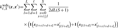(2)

It considers oligomers up to length d, and allows them to be shifted up to S positions, starting from i, in the input sequences. This kernel is better suited for motifs with indels or at varying positions; see e.g. Rätsch et al. (2005) and Sonnenburg et al. (2007a).

The locality improved and oligo kernels by Zien et al. (2000) and Meinicke et al. (2004), respectively, achieve a similar goal in a slightly different way.

2.3 WD kernel with conservation information

To include conservation information, we extended the WDS kernel with a term to multiply the score of the local matches of an oligo of length d at position i with a quantity that depends on its conservation. We propose to use the average conservation of the oligo in pregenerated alignments of sequences from G other organisms:

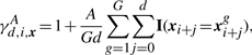(3)

where x^g is the sequence of the syntenic regions in the genome of organism g=1,…, G and A>0 is a parameter allowing one to control the importance of the conservation. We add 1 to not ignore unconserved sequences: ideally, the conservation should only add information by emphasizing the conserved and hence likely functionally important regions of the regulatory sequence. All results shown were obtained with the setting of A=1. Using this definition of a conservation score, we can now define the WD kernel with shifts and conservation (WDSC):

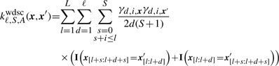(4)

The above kernel, like the WDS kernel, corresponds to a feature space spanned by all possible k-mers at every position. While the feature value is 1 for the WDS kernel if the k-mer is present at a certain position, for the WDSC kernel the feature value is γ_d,i,x, i.e. it is computed depending on the conservation of the k-mer at this position.

2.4 A kernel for regulatory modules

Suppose we are given a set of M motifs ℳ_m, m=1,…, M, which may either come from a database or from a de novo motif detection method. Such motifs are often represented in a way that one can easily scan a given sequence for occurrences of the motif (e.g. as PWMs). In a preprocessing step, we compute the best matching position p_m,x⁽ⁱ⁾ of each motif ℳ_m in all considered sequences x⁽ⁱ⁾, i=1,…, N. In case of PWMs, the PWM score (Schneider et al., 1986) and in case of oligo-based motifs, the Hamming distance may be used to decide which position in the sequence matches best. We use MotifScanner from the inclusive package by Thijs et al. (2002) to scan sequences for the best matching occurrence of a PWM; in case of an oligomer, we use a regular expression pattern with decreasing discriminative power to find the closest match. In case of a tie, the last match in the sequence is selected.

2.4.1 Kernel for multiple motifs

For the kernel functions, all input vectors need to be of the same length. Therefore, we have to choose the same number of matches per sequence for all motifs (1 in our case), regardless of the quality of the matches, as shown in Figure 1. Biologically, a threshold quality seems more intuitive. Then, several good matches would be considered, or no match for sequences that do not contain the motif. However, a soft margin during training allows the algorithm to ignore some mislabeled data points, i.e. sequences that do not contain the motif, without strong effects on generalization. A soft margin SVM uses a slack variable ξ and can tolerate training data points that, e.g. clearly lie in the space of the class they do not belong to without skewing the separating hyperplane in order to correctly classify such outliers. This allows the SVM to separate data that would not be linearly separable when using a hard margin, usually achieves a better classification result due to a ‘smoother’ hyperplane, and makes the SVM more robust against noisy data (Schölkopf and Smola, 2001).

Fig. 1.

The idea behind the RM kernel: a motif finder is applied to the regulatory sequences in the input set (long, dark bars), which identifies overrepresented motifs (short, light bars). The best matching motifs (boxed) in every sequence serve as starting points, where we excise a window of 20 bp around the center of each motif occurrence for the WDSC kernel. Conservation information for these windows is looked up in a precomputed multiple genome alignment (cf. Section S.2 of the Supplementary Material for details on conservation data). Additionally, we construct an input vector for the RBF kernel of the pairwise motif distance, and distance to the transcription start (if available).

Similar ideas have been proposed and successfully used in image analysis, using kernel methods where motifs correspond to points of interest, e.g. sharp edges (Mikolajczyk et al., 2005; Nowak et al., 2006).

The main idea of the kernel that we propose is to represent an input sequence x by the set of sequences x_m≔x_{[pm,x−w,pm,x+w]} originating from the region of length 2w around the best motif match p_m,x of motif ℳ_m in x. Each sequence region x_m contributes independently to the similarity between two input sequences: k₁(x, x′)=∑_m=1^Mk(x_m, x′_m). This term characterizes the co-occurrence of a collection of motifs in two sequences x and x′. The similarity is highest if all motifs appear in both sequences (in arbitrary order). We propose to use a position-specific string kernel, for instance the WDSC kernel, to compute the similarity of the regions.

2.4.2 Modeling positional information

For the first part of the kernel, the position of the motif does not influence the similarity at all, since the motif windows have been extracted from the input sequence. In the second part of the kernel, we try to capture the relative position of the best motif matches to each other and to the transcription start site, if available. This is achieved by computing all pairwise distances between match positions of motifs: v(x)=(p_1,x−p_tss,…, p_M,x−p_tss, p_1,x−p_2,x,…, p_i,x−p_j,x,…, p_M−1,x−p_M,x)^⊤, for all i≠j=1,…, M, where p_tss is the position of the transcription start site in the sequence. A simple way of computing the similarity between two such vectors is to use the radial basis function (RBF) kernel, e.g. Schölkopf and Smola (2002):

where σ is a kernel hyperparameter to be found by model selection.

In the kirmes pipeline (described below), we create one string kernel per motif, with all the windows where the motif occurs as input data and sum them up to a combined kernel, and add an RBF kernel for all pairwise positions. Having both parts of the kernel defined, the question how to combine them remains. We propose to simply add both contributions in the RM kernel:

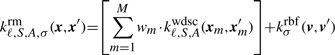(5)

Here, w_m are the weights assigned to the subkernels k^wdsc, which are all set to 1 per default, and x_m is the best match of motif ℳ_m in the sequence x.

Please note that if we add the kernels, it amounts to concatenating the feature spaces. If one multiplied the contributions of distances and motif-sequence similarity, the kernel would be in some sense similar to the previously proposed oligo kernel (Meinicke et al., 2004). In our case, this would not be feasible, since we want to inspect the kernel contributions independently and determine the sequence logo that each string kernel uses to discern the two input classes. Therefore, we want a clear distinction between the contributions of the positional kernel part and the motif part of the kernel.

3 METHODS

3.1 kirmes pipeline

Below, we introduce an integrated python pipeline, called kirmes, using the previously described kernels to classify promoter regions of genes as targets of a certain combination of TFs (i.e. as co-regulated). We outline a use case with a scenario where this pipeline can be applied. DNA sequences considered in the input sets can come from any part of the euchromatin, e.g. upstream and downstream regions of a gene, intronic and exonic parts, as well as untranslated regions (UTR) in the 3′ or 5′ direction, each of arbitrary length. The selection of this region depends on the organism the data stems from; for the use case, we will assume this to be A.thaliana, where good results can be obtained with a combination of upstream, UTR and intronic sequences. We used 1000 bp upstream of the transcription start; in general, longer sequences introduce more noise. In organisms with shorter promoters a reduction would be beneficial for the signal-to-noise ratio.

Figure 2 shows an outline of the pipeline for the classification of promoter sequences based on microarray experiments (cf. Section 3.2).

Fig. 2.

A cartoon workflow of the kirmes pipeline: the preprocessing step requires the genomic sequence and a set of regulatory sequences from genes that were determined to be co-expressed in microarray experiments, and ideally a negative set. kirmes conducts a motif finding step, where it locates the positions of overrepresented motifs in fasta files of the genes' regulatory region. For the classification, we build an input vector with sequence sections of 20 bp, centered around the motif positions obtained during the motif finding step, and optional conservation information from related genome sequences for the WDSC kernel, as described in Section 2.3. The classifier is trained on the labeled dataset of positives and negatives and can then be applied repeatedly on unlabeled prediction datasets to classify genes as co-regulated by the same mechanism as the input dataset or not.

3.1.1 Initial motif finding

In the first step, there is a chocie between several methods to identify candidate motifs. Initially, we used a common Gibbs sampling algorithm (Lawrence et al., 1993) called MotifSampler from the inclusive package by Thijs et al. (2002) that finds overrepresented motifs ℳ_m, m=1,…, M and creates subkernels for up to M motifs. To make sure we do not include motifs that are too common, we use several strategies: first, a background model for this organism; second, minimum occurrences were set to 15 % or three genes of the set, whichever is more; third, 1000 random gene sets were generated and searched for motifs of the same length and determinacy. This was measured through the information content of the position frequency matrix of the motif, an output of the Gibbs sampling program.

Since this last step takes a significant amount of time depending on the length and number of sequences, we searched for alternatives. We settled on one approach, where we count the occurrence of any oligomer of length six in positive sequences (oligo counting). We selected a subset of those oligomers that appear in at least 15% of all positive sequences. This simple strategy certainly leaves room for improvements, but our experiments in Section 3.2 illustrate that it already works rather well.

3.1.2 SVM training

We use the large-scale machine learning toolbox shogun at http://www.shogun-toolbox.org (Sonnenburg et al., 2006) through its python interface. It provides implementations of all kernels described in this work and allows for fast training using several different SVM implementations, e.g. SVM^light (Joachims, 1999). As described in Section 2.4, we create a kernel for every candidate motif ℳ_m and use a window of 20 bp around each occurrence in every sequence. We tested different widths and settled for this length as it gave the highest accurracy for a representative dataset (cf. Supplement S.4 in the Supplementary Material).

3.1.3 Interpretation of results

To find out which of the candidate motifs ℳ_m, m=1,…, M from the initial motif finding step contribute the highest discriminative power of the combined RM kernel k^rmk, we take a look at all the subkernels, each of which describe exactly one motif. Every subkernel has an assigned weight w_m=1 ∀ m=1,…, M, as described in Equation (5). If we iterate over all motifs ℳ_m and in turn set w_m=0, w_i=1 ∀ i≠m once for every motif ℳ_m and re-evaluate the SVM with the combined kernel k^rm\{m} on the same dataset x, we can obtain a ranked list of all motif kernels: we subtract the new training accuracy from the re-evaluation with one of the weights set to 0 (measured in area under the receiver operating characteristic curve, auROC) from the reference accuracy of the combined kernel with all weights set to 1.

This difference gives us the gain in accuracy for just this motif window. The subkernels that contribute the largest difference are the most interesting ones for the experiment, since they contain the strongest candidate binding motif. We then calculate positional oligomer importance matrices developed by Sonnenburg et al. (2008) to obtain a 1mer sequence logo (Schneider and Stephens, 1990) from the kernel that shows the motif that this kernel is attuned to. This ranked list of motifs, along with the auROC difference, allows for a straightforward interpretation of the kirmes prediction results.

3.2 Microarray expression data

We derive sets of co-expressed genes from microarray experiments performed with the commercial Affymetrix GeneChip Arabidopsis ATH1 array. This chip is designed to measure transcript abundance of more than 20 000 genes of the model organism A.thaliana (Redman et al., 2004).

The sets are obtained through a stringent analysis of expression change using the software GeneSpring (Agilent Technologies). We labeled genes as co-expressed when they showed a 4-fold change of expression in the experiment as compared with the control, and considered those genes not co-expressed if their levels remain the same, compared with the control, within a margin of 0.2-fold change. The fold change is computed from the normalized gene expression level p in treatment and respective control, c:

In this case, the direction of the change is represented by the sign of n, positive means up and negative means down relative to the control. If several replicates were available, the mean after normalization is taken for every gene, for all replicates of p and c, respectively.

We used microarray data from two different experimental setups (cf. Section S.1 in the Supplementary Material). The first setup uses leaves from wild type A.thaliana plants exposed to medium at 38^°C versus leaves exposed to the same medium at room temperature, expression measurement taken 1 h after exposure (Busch et al., 2005). The second setup uses inducible overexpression of Arabidopsis meristem regulators with the AlcR/AlcA system. Plants harboring 35S::AlcR/AlcA::GOI (gus control, leafy, shootmeristemless, wuschel) constructs were grown in continuous light for 12 days and induced with 1% ethanol. After 12 h of EtOH treatment, seedlings were dissected and RNA was processed from the shoot apex and from young leaves. Affymetrix ATH1 arrays were hybridized in duplicates for each gene construct and condition (Leibfried et al., 2005). In total, we considered 14 different gene sets to be discriminated by the methods.

3.3 Use case

When a researcher has conducted several microarray experiments and has obtained a list of co-expressed genes that react in concert, ideally over several different experiments, and assumes they are targets of a specific combination of TFs, kirmes can be used to find common motifs in this list and in turn in all other known genes. The experimental design is cruical for the success of our method: kirmes will work best if used on gene sets derived from time-series experiments or from loss or gain of function experiments of a specific gene.

The regulatory sequences of a gene set identified in such a manner have to be available in fasta format. The regulatory region can be anything from promoters, introns, to even the whole chromatin, of arbitrary length, and can stem from any organism. To effectively use the positional information of promoter regions, it is a good idea to select the sequences in such a way that the translation start site is at the same position in each of them.

kirmes assumes that the sequences of regulatory regions are given in two sets: a set enriched with TF targets (labeled positive) and a second set containing no or very few targets (labeled negative). Negative sets could be genes whose expression does not change from the control to the experimental condition, and that are ideally expressed at levels above the microarray detection threshold.

kirmes is available publicly at http://galaxy.fml.mpg.de/, our Galaxy webserver. Galaxy is an open source, scalable framework for tool and data integration developed by Giardine et al. (2005): users can upload their sequence files; kirmes will classify the input gene set and return the names of the co-regulated genes as well as discriminative motifs in a list.

fasta files of sequences can be uploaded to our Galaxy server, where we use the 6mer oligo-counting strategy and the WDS kernel. Conservation information is not supported as it depends on the organism from which the sequences were obtained, it may not always be available and would require a significantly larger infrastructure. There is no upper limit on the amount of input sequences in place, but at least five sequences should be uploaded for cross-validation to work.

In our case, we worked with gene sets from microarray experiments described in Section 3.2. Here, we were looking for a heat shock element identified by Leibfried et al. (2005) as well as a binding motif for the TF wuschel in A.thaliana. We made use of the experimental logic to obtain well-suited gene sets (cf. Section S.1 in the Supplementary Material).

The user working with kirmes can adjust the number of most discriminative motifs to be reported by the program. These motifs are ranked according to their contribution towards class discrimination and are good starting points for further expression or binding validation experiments.

After training of a kirmes classifier, a further prediction dataset can be uploaded. This could for instance be comprised of the same regulatory regions, but this time for all of the annotated genes of this organism. This is especially useful if some newly discovered genes are not yet represented on the microarray platform the expression experiments were performed with, or they were expressed close to the detection threshold and so cannot be readily excluded from the list of genes whose expression was changed in the experiment.

3.4 Experimental setup

To train and test the method and compare it against baseline kernels, we first split the data into two parts (80% : 20%). The first part is used for motif finding and SVM training. For hyperparameter tuning, we used the first part with 5-fold cross-validation to find the optimal combinations of hyperparameters. (The SVM and the considered kernels have several hyperparameters to be given in advance. This includes the regularization parameter C of the SVM, the maximal length of oligomers ℓ and the maximal shift S considered in the WDS kernel.) The second part is used to estimate the generalization performance. Here, we measure the auROC as the generalization performance (random guessing corresponds to 50% auROC).

The above procedure is repeated five times for different splits of training and test examples (outer cross-validation loop). As performance measure, we report the average auROC over the five splits.

To compare our method with the priority algorithm, we used the datasets from yeast chromatin immunoprecipitation experiments on tiling array chips from the extensive study by Harbison et al. (2004). priority was developed by Gordân et al. (2008) and has been applied to this dataset before, but only in comparison to other Gibbs sampling algorithms. We chose this algorithm to compare our method with because it was tested on exactly the kind of data we recommend to be used with kirmes.

The comparison to kirmes is in some ways different to the original setup by Gordân et al. (2008): our method needs labeled information as it is a supervised learning technique. Thus, we employ a 5-fold cross-validation, as described above. To make the conditions as comparable as possible, the unsupervised priority will also see only the same 80% split of sequences to find an overrepresented motif PWM. We search for the top-ranking PWM reported on the training set in the remaining 20% of the positive and negative sequences and calculate the auROC from the distance of the best motif occurrences in the sequences from the reported PWM. This area is compared with the one reported by the cross-validation run of kirmes.

4 RESULTS

The goal is to predict the expression change status of potential target genes for overexpressed TFs based on their promoter sequence, with the datasets and the setup described above.

4.1 Comparison on A.thaliana gene sets

In a first experiment, we illustrate that simple methods, as for instance SVMs with a spectrum or WDS kernel, cannot easily solve the considered classification problem. The results are given in Figure 3A. We can observe that essentially for all gene sets, an SVM with the spectrum kernel fails to identify positive genes (auROC close to 50%). An SVM with the WDS kernel performs slightly better, but still produces close to random predictions.

Fig. 3.

(A) Accuracy of the spectrum and WDS kernels: the prediction is rarely better than random guessing for these kernels. The kernels are not well-suited for this particular problem. The names of the gene sets are derived from the tair7 annotation by the Swarbreck,D. et al. (2007) and are explained in detail in Section S.1 of the Supplementary Material. (B) Accuracy of variations of the kirmes approach: this graph shows a comparison of the basic kernels and the conservation kernels (C) combined with two different motif generation approaches: by oligo-counting (Oligo) or by Gibbs sampling (Gibbs). The average performance (μ) is given for each kernel variant. The first set is taken from a control experiment, where no overrepresented motifs should occur.

In Figure 3B, we present results of the proposed methods in four variants: with motif discovery by Gibbs sampling versus oligo-counting as well as with and without the use of conservation.

We can make the following observations: (i) all four versions show a significantly improved performance relative to the base-line methods. (ii) Motif finding using oligo-counting seems to work considerably better in combination with SVMs than Gibbs sampling, except on the control. A possible reason may be that the number of considered oligos M=100,…, 200 is higher than the number of motifs generated by the Gibbs sampler, M<50. (iii) Using conservation as weighting for the WDS kernel considerably improves the recognition performance. It results in an average performance improvement of 5 percentage points.

4.2 Contribution of vector features

To evaluate the contributions of the individual feature types of the input vectors, we used a representative gene set of the A.thaliana experiments for illustration. We considered different combinations of the feature types of the RM kernel (sequence windows, conservation information and positional information) and observed the classification performance. The results are shown in Figure 4, where each bar corresponds to the auROC after a 5-fold cross-validation with the respective features. We also analyzed other gene sets (data not shown), and observed that the sequence window feature was consistently the most important feature, while positional information in some cases made a big difference, while in other cases its contribution was neglectable. Positional preference or lack thereof has been studied for many TFs, e.g. by Smith et al. (2007) for the cyclic-AMP response element. For this TF, position plays a major role in many reported experiments, but there are cases of functional binding sites that have effects on genes many thousands of base pairs away from the binding site (Smith et al., 2007). Therefore, it is not surprising that for some sequences positional information adds no discriminative power, even within the same gene set, and for others it adds more than 10 percentage points.

Fig. 4.

Comparison between the contributions of each feature type of the input vector. A dataset of 42 positive and 1562 negative genes was used from the A.thaliana experiments.

Conservation always boosts the performance by ≈5 percentage points (cf. Fig. 3).

4.3 Comparison to priority

As described in Section 3.4, we compared kirmes to the state-of-the-art Gibbs sampler priority by Gordân et al. (2008). This setup lets us use priority as a classifier: we measure its performance on a testing set that the Gibbs sampler did not use to build its motif PWM. That way, we can use the top-scoring PWM from the training set and find occurrences in the testing set. The distance to the PWM of each respective best match is scored. This score is used to compute a ROC curve. In Figure 5, we show a box plot on the average auROC of the two approaches on 268 gene sets from Harbison et al. (2004), preprocessed by Raluca Gordân. kirmes is clearly the more accurate classifier, and it can also reveal the motifs it deemed most discriminant.

Fig. 5.

Comparison between the Gibbs sampler priority and the kirmes approach for the task of identifying genes regulated by a TF. The box plot shows the average auROC on the 268 gene sets, giving the minimum, maximum, median, first and third quartile values (cf. Sections 3.4 and 4.3).

5 CONCLUSION

The results clearly illustrate the power of our approach in exploiting the relationship between motifs as well as conservation to improve the recognition of TF targets. All four variants significantly improve the performance over naïve baseline methods. The normalization scheme for the multiple genome alignment can be remodeled to take into account evolutionary distances.

The comparison with priority in Figure 5 shows that kirmes is, not surprisingly, a more accurate classifier than this state-of-the-art Gibbs sampler, because it can make use of several motifs and their positional interdependence. We are not aware of a more similar classification program that uses the same type of original data, against which we could have compared kirmes in lieu of priority.

We chose the Gibbs sampling program MotifSampler in our study because it performed best on the A.thaliana data among four compared Gibbs samplers. It was, however, not included in the comparison of samplers by Gordân et al. (2008). In light of the versatility of kirmes, it would seem pertinent to reinvestigate the performance on a wider selection of data, e.g. by choosing priority as a replacement for the older sampling program or the simplistic oligo-counting method.

For practical purposes, the kirmes algorithm can be applied to any combination of regulatory regions and also any organism. A researcher may use kirmes to filter gene sets obtained through statistical methods from expression or binding data. These sets are usually generated when evaluating microarray expression or binding data, e.g. from analyzing a regulatory network around a TF. Careful experimental design will lead to very concise predictions.

Use of the web service integrated into Galaxy is straightforward and the resulting classification may help to select genes that should be investigated further. kirmes can visualize the central motifs and the area surrounding them that were most discriminant during classification; this output can serve as a starting point for researchers wanting to investigate the regulatory mechanism that drives the expression changes in the experiments they have conducted. The output is more valuable than the one shown by a Gibbs sampling algorithm, because the surrounding regions describe the regulatory module to greater detail than the original 6mer would. Even for experiments where very complex regulatory mechanisms are suspected, kirmes will report at least dominant signatures of the most prevalent mechanism. Here, careful experimental design and time-series experiments can help to untangle more complex relationships. In that sense, using kirmes is not the final solution when trying to understand regulation, but a tool that can be used to direct the design of further validation experiments.

The use by experimentalists will ultimately determine the utility of this approach and govern the direction of further extensions together with technological advances such as next-generation sequencing methods for transcriptome or protein binding data, or its application to other motif-driven biological processes like alternative splicing.

REFERENCES

- Bailey T, Elkan C. Proceedings of ISMB'94. Vol. 2. Menlo Park, CA, USA, ISCB: AAAI Press; 1994. Fitting a mixture model by expectation maximization to discover motifs in biopolymers; pp. 28–36. [PubMed] [Google Scholar]
- Ben-Hur A, et al. Support vector machines and kernels for computational biology. PLoS Comput. Biol. 2008;4:e1000173. doi: 10.1371/journal.pcbi.1000173. [DOI] [PMC free article] [PubMed] [Google Scholar]
- Boser B, et al. Proceedings COLT '92. Pittsburgh, Pennsylvania: ACM Press; 1992. A training algorithm for optimal margin classifiers; pp. 144–152. [Google Scholar]
- Busch W, et al. Identification of novel heat shock factor-dependent genes and biochemical pathways in A. thaliana. Plant J. 2005;41:1–14. doi: 10.1111/j.1365-313X.2004.02272.x. [DOI] [PubMed] [Google Scholar]
- Frith M, et al. Discovering sequence motifs with arbitrary insertions and deletions. PLoS Comput. Biol. 2008;4:e1000071. doi: 10.1371/journal.pcbi.1000071. [DOI] [PMC free article] [PubMed] [Google Scholar]
- Giardine B, et al. Galaxy: a platform for interactive large-scale genome analysis. Genome Res. 2005;15:1451–1455. doi: 10.1101/gr.4086505. [DOI] [PMC free article] [PubMed] [Google Scholar]
- Gordân R, et al. A fast, alignment-free, conservation-based method for transcription factor binding site discovery. In: Vingron M, Wong L, editors. Lecture Notes in Computer Science: RECOMB 2008. Vol. 4955. Heidelberg: Springer; 2008. pp. 98–111. [Google Scholar]
- Gupta M, Liu J. De novo cis-regulatory module elicitation for eukaryotic genomes. Proc. Natl Acad. Sci. USA. 2005;102:7079–7084. doi: 10.1073/pnas.0408743102. [DOI] [PMC free article] [PubMed] [Google Scholar]
- Harbison C, et al. Transcriptional regulatory code of a eukaryotic genome. Nature. 2004;431:99–104. doi: 10.1038/nature02800. [DOI] [PMC free article] [PubMed] [Google Scholar]
- Joachims T. Making large-scale SVM learning practical. In: Schölkopf B, et al., editors. Advances in Kernel Methods - Support Vector Learning. Cambridge, MA: MIT Press; 1999. [Google Scholar]
- Lawrence CE, et al. Detecting subtle sequence signals: a Gibbs sampling strategy for multiple alignment. Science. 1993;262:208–214. doi: 10.1126/science.8211139. [DOI] [PubMed] [Google Scholar]
- Leibfried A, et al. Wuschel controls meristem function by direct regulation of cytokinin-inducible response regulators. Nature. 2005;438:1172–1175. doi: 10.1038/nature04270. [DOI] [PubMed] [Google Scholar]
- Leslie C, et al. Proceedings of the Pacific Symposium on Biocomputing. New Jersey, London, Singapore, Beijing, Shanghai, Hong Kong, Taipei: World Scientific; 2002. The spectrum kernel: a string kernel for SVM protein classification; pp. 564–575. [PubMed] [Google Scholar]
- Leslie C, et al. Mismatch string kernels for discriminative protein classification. Bioinformatics. 2003;20:467–476. doi: 10.1093/bioinformatics/btg431. [DOI] [PubMed] [Google Scholar]
- Matys V, et al. Transfac: transcriptional regulation, from patterns to profiles. Nucleic Acids Res. 2003;31:374–378. doi: 10.1093/nar/gkg108. [DOI] [PMC free article] [PubMed] [Google Scholar]
- Meinicke P, et al. Oligo kernels for datamining on biological sequences: a case study on prokaryotic translation initiation sites. BMC Bioinformatics. 2004;5:169. doi: 10.1186/1471-2105-5-169. [DOI] [PMC free article] [PubMed] [Google Scholar]
- Mikolajczyk K, et al. A comparison of affine region detectors. Int. J. Comput. Vis. 2005;65:43–72. [Google Scholar]
- Müller K, et al. An introduction to kernel-based learning algorithms. IEEE Trans. Neural Netw. 2001;12:181–201. doi: 10.1109/72.914517. [DOI] [PubMed] [Google Scholar]
- Noble W. What is a support vector machine? Nat. Biotechnol. 2006;12:1565–1567. doi: 10.1038/nbt1206-1565. [DOI] [PubMed] [Google Scholar]
- Nowak E, et al. European Conference on Computer Vision. Heidelberg: Springer; 2006. Sampling strategies for bag-of-features image classification. [Google Scholar]
- Rätsch G, Sonnenburg S. Accurate splice site detection for Caenorhabditis elegans. In: Schölkopf KTB, Vert J-P, editors. Kernel Methods in Computational Biology. Cambridge, MA, USA: MIT Press; 2004. pp. 277–298. [Google Scholar]
- Rätsch G, et al. RASE: recognition of alternatively spliced exons in C. elegans. Bioinformatics. 2005;21(Suppl. 1):i369–i377. doi: 10.1093/bioinformatics/bti1053. [DOI] [PubMed] [Google Scholar]
- Redman J, et al. Development and evaluation of an Arabidopsis whole genome affymetrix probe array. Plant J. 2004;38:545–561. doi: 10.1111/j.1365-313X.2004.02061.x. [DOI] [PubMed] [Google Scholar]
- Sandelin A, et al. Jaspar: an open-access database for eukaryotic transcription factor binding profiles. Nucleic Acids Res. 2004;32:D91–D94. doi: 10.1093/nar/gkh012. [DOI] [PMC free article] [PubMed] [Google Scholar]
- Schneider TD, Stephens RM. Sequence logos: a new way to display consensus sequences. Nucleic Acids Res. 1990;18:6097–6100. doi: 10.1093/nar/18.20.6097. [DOI] [PMC free article] [PubMed] [Google Scholar]
- Schneider TD, et al. Information content of binding sites on nucleotide sequences. J. Mol. Biol. 1986;188:415–431. doi: 10.1016/0022-2836(86)90165-8. [DOI] [PubMed] [Google Scholar]
- Schölkopf B, Smola AJ. Learning with Kernels: Support Vector Machines, Regularization, Optimization, and Beyond. Cambridge, MA: MIT Press; 2001. [Google Scholar]
- Schölkopf B, Smola A. Learning with Kernels. Cambridge, MA: MIT Press; 2002. [Google Scholar]
- Schölkopf B, et al. Kernel Methods In Computational Biology. Cambridge, MA: MIT Press; 2004. [Google Scholar]
- Segal E, Sharan R. A discriminative model for identifying spatial cis-regulatory modules. J. Comput. Biol. 2005;12:822–834. doi: 10.1089/cmb.2005.12.822. [DOI] [PubMed] [Google Scholar]
- Sinha S, Tompa M. Discovery of novel transcription factor binding sites by statistical overrepresentation. Nucleic Acids Res. 2002;30:5549–5560. doi: 10.1093/nar/gkf669. [DOI] [PMC free article] [PubMed] [Google Scholar]
- Smith B, et al. Evolution of motif variants and positional bias of the cyclic-amp response element. BMC Evol. Biol. 2007;7(Suppl. 1):S15. doi: 10.1186/1471-2148-7-S1-S15. [DOI] [PMC free article] [PubMed] [Google Scholar]
- Sonnenburg S, et al. Large scale multiple kernel learning. J. Mach. Learn. Res. 2006;7:1531–1565. [Google Scholar]
- Sonnenburg S, et al. Accurate splice site prediction using support vector machines. BMC Bioinformatics. 2007a;8(Suppl. 10):S7. doi: 10.1186/1471-2105-8-S10-S7. [DOI] [PMC free article] [PubMed] [Google Scholar]
- Sonnenburg S, et al. Large scale learning with string kernels. In: Bottou L, et al., editors. Large Scale Kernel Machines. Cambridge, MA, USA: MIT Press; 2007b. pp. 73–104. [Google Scholar]
- Sonnenburg S, et al. POIMs: positional oligomer importance matrices–understanding support vector machine-based signal detectors. Bioinformatics. 2008;24:6–14. doi: 10.1093/bioinformatics/btn170. [DOI] [PMC free article] [PubMed] [Google Scholar]
- Stormo GD. DNA binding sites: representation and discovery. Bioinformatics. 2000;16:16–23. doi: 10.1093/bioinformatics/16.1.16. [DOI] [PubMed] [Google Scholar]
- Swarbreck D, et al. The Arabidopsis Information Resource (TAIR): gene structure and function annotation. Nucleic Acids Res. 2007;36(Database issue):D1009–D1014. doi: 10.1093/nar/gkm965. [DOI] [PMC free article] [PubMed] [Google Scholar]
- Thijs G, et al. Inclusive: integrated clustering, upstream sequence retrieval and motif sampling. Bioinformatics. 2002;18:331–332. doi: 10.1093/bioinformatics/18.2.331. [DOI] [PubMed] [Google Scholar]
- Yada T, et al. Automatic extraction of motifs represented in the hidden Markov model from a number of DNA sequences. Bioinformatics. 1998;14:317–325. doi: 10.1093/bioinformatics/14.4.317. [DOI] [PubMed] [Google Scholar]
- Zien A, et al. Engineering support vector machine kernels that recognize translation initiation sites. Bioinformatics. 2000;16:799–807. doi: 10.1093/bioinformatics/16.9.799. [DOI] [PubMed] [Google Scholar]