

Abstract
Stereotaxic atlases of the mouse brain are important in neuroscience research for targeting of specific internal brain structures during surgical operations. The effectiveness of stereotaxic surgery depends on accurate mapping of the brain structures relative to landmarks on the skull. During postnatal development in the mouse, rapid growth-related changes in the brain occur concurrently with growth of bony plates at the cranial sutures, therefore adult mouse brain atlases cannot be used to precisely guide stereotaxis in developing brains. In this study, three-dimensional stereotaxic atlases of C57BL/6J mouse brains at six postnatal developmental stages: P7, P14, P21, P28, P63 and in adults (P140–P160) were developed, using diffusion tensor imaging (DTI) and micro-computed tomography (CT). At present, most widely-used stereotaxic atlases of the mouse brain are based on histology, but the anatomical fidelity of ex vivo atlases to in vivo mouse brains has not been evaluated previously. To account for ex vivo tissue distortion due to fixation as well as individual variability in the brain, we developed a population-averaged in vivo MRI adult mouse brain stereotaxic atlas, and a distortion-corrected DTI atlas was generated by nonlinearly warping ex vivo data to the population-averaged in vivo atlas. These atlas resources were developed and made available through a new software user-interface with the objective of improving the accuracy of targeting brain structures during stereotaxic surgery in developing and adult C57BL/6J mouse brains.
Keywords: brain, stereotaxic atlas, diffusion tensor MRI, micro-CT, mouse
Atlases of the mouse brain are fundamentally important in various types of neuroscience studies, including identification of specific brain regions, guidance of stereotaxic operations, and registration of information such as gene expression locations. In the past, histology-based atlases of rodent brains have been widely used for these purposes (Sidman et al., 1971; Pellegrino et al., 1979; Paxinos and Watson, 1982; Kaufman, 1992; Kruger et al., 1995; Franklin and Paxinos, 1997; Jacobowitz and Abbott, 1997; Hof et al., 2000; Baldock et al., 2001; Valverde, 2004; Paxinos et al., 2007; Dong, 2008; Schambra, 2008). Among these applications of the atlases, stereotaxic surgical operations such as injection of chemical substances, implantation of electrodes, site-targeted cell delivery and irradiation, require knowledge of the accurate coordinates of brain structures of interest. Stereotaxic surgery in the mouse is based on the assumption that structures within the brain can be precisely and reliably located with respect to external skull landmarks (Slotnick and Leonard, 1975; Athos and Storm, 2001). Currently, the Franklin and Paxinos atlas (2008) and the Allen Institute atlases (Lein et al., 2007; Dong, 2008) offer such stereotaxic coordinates for C57BL/6J adult mouse brains. There are, however, several limitations in using these histology-based atlases. The first issue is coordinate accuracy. Brain coordinates need to be defined relative to external skull features such as the bregma or the lambda junction. For histological staining, the brain has to be dissected out from the skull, and since the skull and brain tissue are examined separately, there is a prospect of misalignment. The procedures of specimen fixation, sectioning and staining involved in histological processing can induce deformation of the tissue sample, which is another source of significant inaccuracy. Second, histology-based atlases are inherently two-dimensional. This makes it extremely difficult to design a needle path at an oblique angle to avoid damaging important structures of interest. Third, to the best of our knowledge, there is currently no widely available stereotaxic atlas of developing postnatal mouse brains.
In the past, several excellent magnetic resonance imaging (MRI)-based atlases of adult (Benveniste et al., 2000; MacKenzie-Graham et al., 2004; Kovacevic et al., 2005; Dorr et al., 2008), as well as developing (Jacobs et al., 1999; Dhenain et al., 2001; Lee et al., 2005; Ma et al., 2005; Ma et al., 2008) mouse brains have been introduced. The advantage of MRI atlases is clear. They are three-dimensional and, without the sectioning process, have much less anatomical deformation. There are also MRI-based mouse atlases with detailed segmentations (Ali et al., 2005; Bock et al., 2006; Badea et al., 2007; Dorr et al., 2008; Ma et al., 2008; Sharief et al., 2008). However, MRI has limited value for visualizing skull structures, which is necessary to establish skull-based stereotaxic coordinates. Recently, Chan et al. (2007) published the first micro-computed tomography (CT) and MRI combined atlas of the adult C57BL/6J mouse brain. In our study, we extended these atlases in several respects. First, we developed stereotaxic atlases for six different developmental stages of the C57BL/6J mouse, starting from postnatal day 7 (P7). During the early postnatal period, rapid age-related morphological changes in the brain occur concurrently with the growth of bony plates at the cranial sutures (Zimmermann et al., 1998). The most obvious postnatal changes relate to myelination (Barbarese et al., 1978; Carson et al., 1983; Vincze et al., 2008) which begins in the mouse spinal cord on about the day of birth, and then advances into the mouse brain more or less progressively in the rostral direction beginning at about P10, proceeding rapidly from P10–P30 with a peak rate of formation at about P17, then progressing at a slower rate from P30–P60 and probably continuing at a very slow rate thereafter. Due to the changing spatial relationships between the brain and the overlying skull structures during development, adult mouse brain atlases cannot be used to guide stereotaxic operations in early postnatal subjects. Second, we performed diffusion tensor imaging (DTI) (Basser et al., 1994) to obtain satisfactory tissue contrasts in early postnatal mouse brains. During early postnatal development, brains are not fully myelinated; and since conventional MRI contrasts rely mostly on tissue myelin content, these brains look relatively homogeneous, so that it is difficult to identify specific brain structures. As shown in past studies by our group and others (Mori et al., 2001; Verma et al., 2005; Zhang et al., 2005; Chahboune et al., 2007; Larvaron et al., 2007; Baloch et al., 2009), DTI can provide superior contrasts to delineate neuroanatomy in these brains. Third, for the adult atlas, we attempted to increase the accuracy of structural coordinates by incorporating population-averaged anatomy of in vivo adult mouse brains, in order to correct for tissue distortion caused by fixation and to avoid any sample-specific bias in the definition of anatomical structures associated with the single-subject atlas. A user-interface was developed for use of these 3D MRI-CT atlases to guide stereotaxic operations.
Our atlas is still not comprehensive in terms of coverage of ages, gender, population size, annotation, and segmentation. The format requirement of the atlases may vary depending on how these atlases will be used. To enhance further development of more comprehensive atlases, our database will be open to the public at our website (http://lbam.med.jhmi.edu). In this paper, we describe the details of our atlas construction, and compare stereotaxic coordinate locations of adult C57BL/6J brain structures provided by our MRI-CT atlas with the existing widely-used histology-based atlases.
Experimental Procedures
Animal samples
All experimental procedures performed conformed to the animal care guidelines by NIH and the Animal Research Committee at the Johns Hopkins University School of Medicine. C57BL/6J mice at six different developmental stages: postnatal day 7 (P7), P14, P21, P28, P63, and adult (P140–160) were used to construct the stereotaxic atlases. The number of samples used for in vivo MRI, ex vivo MRI, and CT scanning are listed in Table 1. Among these samples, 5 adult brains were each imaged for all of CT, in vivo and ex vivo MRI. Mice were perfusion-fixed with 4% paraformaldehyde in 0.1 M phosphate buffer by transcardial perfusion, followed by removal and immersion fixation of brain specimens within the intact skulls for four weeks. Prior to imaging, the specimens were placed in PBS for more than 24 hours to wash out the fixation solution and then transferred to home-built glass tubes for MR imaging. The tubes were filled with fomblin (Fomblin Profludropolyether, Ausimont, Thorofare, NJ, USA) to prevent dehydration.
Table 1.
The number of animal samples used for CT, ex vivo MRI and in vivo MRI studies
| Age | P7 | P14 | P21 | P28 | P63 | >P140* |
|---|---|---|---|---|---|---|
| Micro CT | 1 | 1 | 1 | 1 | 1 | 8 (5) |
| Ex vivo MRI | 1 | 1 | 1 | 1 | 1 | 10 (5) |
| In vivo MRI | 0 | 0 | 0 | 0 | 0 | 9 (5) |
Figures in parentheses indicate the number of samples imaged with all of CT, ex vivo and in vivo MRI, and used for construction of the population-averaged stereotaxic atlas of the adult mouse brain.
In vivo MRI
In vivo T2-weighted MRI of 9 adult mice was performed with a Bruker 400 MHz (9.4 T) spectrometer. Mice were anesthetized using 1% isoflurane mixed with air and oxygen at a 3:1 ratio. Respiration was monitored via a small animal monitoring system. The respiratory rate was maintained at approximately 80 breaths per minute by adjusting the amount of isoflurane. A 3D T2-weighted fast spin echo sequence with navigator-echo phase correction scheme (Mori and van Zijl, 1998) was used with 4 spin echoes, echo time (TE) of 35 ms, repetition time (TR) of 700 ms and two signal averages. The acquired imaging matrix size was 210 × 120 × 80, and the k-space data were zero-filled to twice the size of the original matrix, to give an image resolution of 0.050 mm × 0.050 mm × 0.125 mm. The total imaging time was about 1 hour for each animal.
Ex vivo MRI
Ex vivo imaging was performed with an 11.7 T NMR spectrometer (Bruker BioSpin, Billerica, MA, USA). The gradient system (Micro 2.5, Bruker Biospin) was calibrated by a phantom with known physical dimensions. Bird-cage RF coils of 15–20 mm diameter were used for transmitting and receiving. Images were acquired using a 3D diffusion-weighted multiple spin echo sequence with 4 spin echoes, TE/TR = 35/550 ms and two signal averages. The imaging matrices and fields-of-view were varied within the range of 150 × 96 × 86 to 186 × 100 × 76 and 17 mm × 11 mm × 9.8 mm to 23 mm × 12.4 mm × 9.4 mm, respectively, depending on the size of the heads. The spectral data were apodized by a 10% trapezoidal function and zero-filled to give a nominal resolution of 62.5 × 62.5 × 62.5 μm3. For DTI of each sample, two non diffusion-weighted and six diffusion-weighted images (b value ~1600–1800 s/mm2) were acquired with δ = 6 ms and Δ= 14 ms. Diffusion sensitizing gradients were applied along six non-collinear directions: [0.707, 0.707, 0], [0.707, 0, 0.707], [0, 0.707, 0.707], [−0.707, 0.707, 0], [0.707, 0, −0.707], [0, −0.707, 0.707]. The total imaging time was approximately 24 hours for each sample. The diffusion tensor was calculated by a multivariate linear fitting method, and diagonalized to obtain three pairs of eigenvalues and corresponding eigenvectors. For quantification of diffusion anisotropy, we used fractional anisotropy (FA) and Westin’s linear anisotropy (CL) (Westin et al., 2002). Color map images were computed from the primary eigenvector and CL images. For each voxel, the ratio between the red, green and blue components was defined by the ratio of absolute values of x, y and z components of the primary eigenvector, and the intensity was proportional to CL. Red was assigned to the medial-lateral direction, green to the rostral-caudal, and blue to the dorsal-ventral direction.
In addition to DTI, high-resolution T2-weighted images were also acquired with the same field of view and resolution, using a 3D fast spin echo sequence with an echo train length of 4, flip angle of 40 degrees, TE/TR = 40/800 ms, four signal averages and imaging time of 3 hours per sample.
Micro-CT
Micro-CT of the mouse heads was performed with a SkyScan 1172 micro-CT system (Micro Photonics Inc., Allentown, PA, USA), with the source biased at 70kV/141μA and an Al-0.5 mm filter to reduce beam hardening. The images were acquired at a pixel size of 18.16 μm, with the camera to source distance 217 mm, and the object to source distance 83 mm. A 0.4° rotation step was used through 180° and 6 frames were averaged together at each rotation step with an exposure time of 158 ms per frame. The scan duration was about 15 minutes for each sample.
Fusion of MRI and CT data
Once the anatomy of the nervous system tissue is characterized either by ex vivo (early postnatal brains) or ex vivo/in vivo (adult brains) MR imaging, the next important step is the fusion of the MRI and CT data.
To develop an atlas for stereotaxic purposes, the CT images of the mouse skull at each developmental stage were co-registered with the MR images. As the first step, landmark-based rigid registration was used for spatial alignment of the CT and MR datasets. Several anatomical landmarks were manually defined on the micro-CT skull images with the Landmarker software (www.mristudio.org) (Zhang et al., 2009), and corresponding landmarks were then identified on the MR images. The anatomical landmarks used for registration were selected such that they could be reliably identified on both the CT and MR images. A rigid transformation model with six degrees of freedom was then used to spatially align the two datasets. Next, the bregma and lambda junctions were identified on the skull images, and the coregistered MRI-CT images were then spatially reoriented using a rigid transformation such that the height of the dorsal skull surface at the bregma and lambda landmarks would be the same (bregma – lambda horizontal), according to the standard orientation defined in the Paxinos murine atlases (Paxinos and Watson, 1982; Franklin and Paxinos, 2008).
Population-averaged adult mouse brain anatomy and estimation of the degree of anatomical variability
We used the in vivo imaging data of the adult mouse population (n = 9) to create an averaged brain anatomical template. First, we chose one of the mouse brains with median brain volume as the reference brain (R0). All other brain images were intensity-normalized (using a piece-wise linear function to equalize the mean intensities of the gray and white matter regions across all brain images), and then rigidly aligned to the reference brain, to match the spatial location and orientation. These aligned brain images were intensity-averaged voxel-wise to create the first population-averaged brain (1st reference, R1). The R1 brain was used as a template for affine (12-mode linear) transformation of the rigidly aligned images. These affine transformed images were averaged to generate the 2nd reference (R2), which was then used as the new template for affine transformation. This process was repeated iteratively five times to generate the 5th reference brain (R5), which was used as the template for non-linear transformation of all in vivo images, based on Large Deformation Diffeomorphic Metric Mapping (LDDMM) (Miller et al., 2002). LDDMM generates diffeomorphic transformations, which are differentiable transformations with differentiable inverses. The diffeomorphism is estimated as the end point of the flow of a velocity vector field, and can accurately map one brain image to another such that the topological relationships of anatomical structures are preserved under the mapping, so that connected structures remain connected, disjoint structures remain disjoint, and substructures are preserved. The diffeomorphism is especially important for mapping tensor images since it ensures that the transformed diffusion tensors remain positive definite. After LDDMM, the deformed images were averaged to create the final in vivo population-averaged atlas (called “master atlas” hereafter). Transformations generated by LDDMM record the quantitative differences between the template and each mouse brain at every voxel. For a given template coordinate [x, y, z]template, a deformation vector [Δx, Δy, Δz]template-sample was obtained for each sample. By averaging the length of the deformation vectors for the 9 mice at each voxel, the anatomical variability magnitude map (AVM) was obtained.
Correction of adult ex vivo atlas
While ex vivo imaging can provide high-resolution images with various contrasts, there are two possible sources of inaccuracy. First, the anatomical fidelity could be compromised by fixation-related tissue deformation. Second, because the ex vivo atlas is based on a single mouse brain, it may include bias due to sample-specific anatomical features. To minimize these effects, we used the in vivo-based master atlas and warped a high-resolution ex vivo image non-linearly to the master atlas. The population-averaged in vivo T2-weighted image was used as the template and the ex vivo T2-weighted image was non-linearly registered to the template. To enable precise region-to-region mapping, the images were first intensity-normalized using a piece-wise linear function to equalize the mean intensities of the grey matter, white matter and cerebrospinal fluid regions in the brain. The ex vivo image was registered to the in vivo master atlas using a rigid transformation, followed by nonlinear warping using LDDMM. The resultant transformation was then applied to the diffusion tensor to create a high-resolution ex vivo DTI atlas of the adult mouse brain in the master template space (simply a “distortion-corrected ex vivo atlas” hereafter). The transformation of the tensor field was carried out by the method proposed by Alexander et al. (Alexander et al., 2001; Xu et al., 2003).
Results
Micro-CT of developing brains
High resolution micro-CT of the developing mouse skull enabled three-dimensional visualization of the bone structures and identification of the cranial sutures and prominent skull landmarks. Fig. 1 shows the three dimensional reconstructions of mouse skulls from micro-CT images at six time points: P7, P14, P21, P28, P63 and adult (P140). To establish the stereotaxic coordinate frame, two anatomical landmarks were identified on each skull: the bregma junction (the point of intersection of the posterior frontal, sagittal and coronal sutures), and the lambda junction (the point of intersection of the lamboid and sagittal sutures). The lambda junction was defined as the point of intersection of the best fit lines passing through the sagittal and lamboid sutures, as in the Franklin and Paxinos atlas. During early stages of postnatal development of the mouse skull, there is rapid ongoing appositional growth along the suture margins leading to progressive narrowing of the sutures (Zimmermann et al., 1998). Therefore, at postnatal day 7, limited ossification of the neurocranium and existence of wide sagittal and lamboid sutures (Fig. 1, P7) made it difficult to define accurately the positions of the bregma and lambda landmarks. The cranial landmarks defined on the adult mouse skull (Fig. 1, P140) were used to measure the size of the skulls (Table 2).
Figure 1.

Three dimensional reconstruction of micro-CT images showing the dorsal view of the mouse skull at six developmental stages from P7 to P140. Cranial landmarks used to measure the skull dimensions are defined on the P140 skull image: nasion (1), bregma (2), lambda (3), intersection of the occipital and interparietal bones at the midline (4), left and right intersection of the parietal, temporal and occipital bones (5, 6).
Table 2.
Basic dimensions of the skull and the brain of C57BL/6J adult mice measured by CT, ex vivo MRI, and in vivo MRI
| Skull | Length1 | Width2 | Height3 | B-L distance4 |
|---|---|---|---|---|
| CT | 14.75 ± 0.08 | 9.91 ± 0.09 | 6.71 ± 0.13 | 4.13 ± 0.05 |
| Brain | Length5 | Width6 | Height7 | Volume8 |
| Ex vivo MRI | 14.53 ± 0.18 | 9.96 ± 0.07 | 6.13 ± 0.10 | 454.43 ± 12.48 |
| In vivo MRI | 14.86 ± 0.14 | 10.10 ± 0.07 | 6.20 ± 0.08 | 472.85 ± 11.56 |
| % shrinkage | 2.2 ± 0.8 | 1.4 ± 0.8 | 1.1 ± 0.6 | 3.8 ± 0.6 |
Distance between landmarks 1 and 4 in Fig. 1.
Distance between landmarks 5 and 6 in Fig. 1.
Maximum dorsal-ventral distance in the bregma coronal plane of the skull, after bregma-lambda horizontal alignment.
Bregma-Lambda distance (between landmarks 2 and 3 in Fig. 1).
Distance between the tip of the olfactory bulb and the posterior edge of the cerebellum.
Left-right width at the widest coronal section of the brain.
Maximum dorsal-ventral distance in the brain, after registration of the brain to the bregma-lambda horizontally oriented skull.
Brain tissue volume from the anterior edge of the olfactory bulb to the posterior edge of the cerebellum.
Single-subject MRI-CT combined images of developing brains
To construct the single-subject stereotaxic surgical atlases of developing mouse brains, the micro-CT and MRI datasets were co-registered using the landmark-based rigid registration approach described above. Fig. 2 shows the results of co-registration of the CT and MR images for C57BL/6J mice at P7, P14, P21, P28 and adult (P140). For each stage, the mid-sagittal section and a coronal section are shown. Micro-CT skull images are shown as a metallic color map overlaid on gray-scale diffusion-weighted images. Color map images generated from CL and the principle eigenvector directions are also shown in Fig. 2. In conventional T2-weighted and average diffusion-weighted images, the overall brain and ventricle boundaries can be clearly delineated, and several structures of interest in stereotaxic operations can be identified. However, during the early stages of postnatal development (before P28), due to incomplete myelination in the brain, conventional MR images often appear homogeneous, and delineation of structures in these images can be challenging. DTI provides superior contrasts for demarcation of brain structures even in these early postnatal brains. This can be seen in the color-coded coronal maps derived from DTI (Fig. 2, third column), where major gray and white matter structures can be clearly identified throughout the development process.
Figure 2.

Co-registered CT and MRI sections from single-subject C57BL/6J mouse brain images from P7 to adult. CT skull images (in metallic color) are overlaid on grey-scale average diffusion-weighted MR images of the brain. For each time point, the mid-sagittal sections are shown in the first column, and a coronal section in the second column. In the third column, the same coronal sections are shown in color-coded orientation maps derived from DTI.
User-interface of the MRI-CT atlases
The atlas consists of high-resolution mouse brain images with micro-CT and multiple MR contrasts (T2-weighted, diffusion-weighted, fractional anisotropy and color-coded orientation maps) at each of the six postnatal stages. The bregma landmark on the dorsal skull surface was chosen as the origin of the coordinate system, and the y-axis was defined along the bregma-lambda horizontal line. Thus, in our atlas database the y-coordinate represents the distance from bregma along the rostral-caudal orientation, while the x- and z-coordinates represent the distances from bregma along the medial-lateral and dorsal-ventral directions, respectively.
The 3D viewing software “AtlasView” (H. Jiang and S. Mori, http://lbam.med.jhmi.edu) was developed to provide a user-interface for navigation through the different imaging contrasts. Fig. 3 shows the AtlasView interface that can be used to directly read the stereotaxic coordinates of any location within the brain, relative to the origin. We chose bregma as the origin of the coordinate frame, but in this software the user can define the origin at bregma, lambda, interaural line, or any other user-defined point. Once a structure of interest is identified, its coordinates can be directly read by moving the cursor to the structure location, and used for stereotaxic operations. The brain anatomy can be inspected three-dimensionally, with a 3D re-orientation capability. AtlasView can dynamically rotate and reslice the atlases (Fig. 3B), which could be an important function if the mouse head is not fixed in the bregma-lambda flat position (the standard orientation adopted in many stereotaxic atlases), and the atlas needs to be rotated to the corresponding orientation. AtlasView also has an interface to visualize pre-defined 3D anatomical structures to aid in understanding the spatial relationships of an intended needle trajectory with the surrounding brain anatomy. This enables designing an oblique injection path to target a particular region of interest without damaging important adjoining structures. Fig. 3A illustrates an example of one of the functions that allows the user to visualize a hypothetical needle path by specifying the needle coordinates (X, Y and Z translation) and the angle of tilt about the X axis with respect to the anatomical landmark chosen as the origin. These functions would significantly enhance our ability for pre-operative planning of needle paths. The AtlasView software, image database, and list of segmented structures can be downloaded at http://lbam.med.jhmi.edu.
Figure 3.

User interface of the AtlasView visualization software, that enables navigation through CT and different MR contrasts in the mouse atlas with three orthogonal views, and also allows 3D rotation and extraction of oblique slices. Pre-defined anatomical structures are listed, which can be chosen for 3D and 2D visualization. In this figure, the caudoputamen (green), the thalamus (yellow), and hippocampus (red) are shown. A) 1: 3D Rotation and oblique slice extraction. 2: Grid selection for stereotaxic coordinate display. 3: CT or different MRI contrast selection. 4: Pre-defined anatomical structures. 5: Selection of coordinate origin. The origin can be specified at bregma, lambda, interaural line or a user-defined point. 6: Interface for visualization of a hypothetical needle path, by specifying the needle translation and angles of tilt and rotation. In this example, the needle (shown in red) is targeting the thalamus without hitting the hippocampus and caudoputamen. 7: Stereotaxic coordinates of any region can be read directly by moving the cursor to that location. B) Oblique slice extraction after the atlas is rotated by 10 degrees about the medial-lateral axis. The rotated brain position can be appreciated in the sagittal view and the coronal view shows a re-sliced section based on the new orientation. The new coordinates are established in the rotated brain position as shown in the grid.
Population-averaged anatomy of the adult mouse brain and characterization of anatomical variability
For the adult mouse brain, a 2nd level atlas was developed, in which we attempted to answer important questions related to atlas accuracy, i.e. tissue deformation due to fixation and the degree of anatomical variability. In Table 2, the overall anatomical dimensions of the adult skull and brain based on CT, in vivo, and ex vivo MRI are tabulated.
To evaluate the degree of anatomical variability, we first created a population-averaged master atlas for the adult mouse brain based on the 9 in vivo MRI datasets (Fig. 4A). This master atlas was designed to be unbiased and to represent the “average” anatomy within the sample population by the procedure described in the Methods section. A deformation map was then computed for each subject by mapping individual brain MRI data to this master atlas. The deformation vector gives the displacement of each voxel under the warping (shape matching between the individual data and the master atlas), which quantitatively measures the anatomical differences. The variability map (AVM) obtained by averaging the magnitude of the deformation vectors at every voxel location in the brain is shown in Fig. 4B. Grey-scale intensity levels in the AVM denote distances in micrometers, and represent the average anatomical variability in the adult mouse brain across the sample population used in this study. The highest degree of variability across subjects, as much as 0.21 mm, was seen in the olfactory bulb and brainstem regions. Tissues around the lateral ventricles also tended to have large variability (up to 0.16 mm). The average spatial variability in the whole brain was calculated to be 0.10 ± 0.03 mm.
Figure 4.

The 2nd level shrinkage- and distortion-corrected atlas of the adult C57BL/6J mouse brain. (A) Population-averaged in vivo ‘master’ atlas of the C57BL/6J brain. Three orthogonal sections are shown, with contours outlining the overall brain volume and the ventricular volume. (B) The anatomical variability magnitude map (AVM) of the sections in panel A. The grey scale intensities represent distances in micrometers. (C) The distortion-corrected ex vivo atlas after warping to the in vivo master atlas. The contour lines of the in vivo atlas are overlaid on T2-weighted images of the corrected ex vivo atlas. (D) Coronal sections from the corrected ex vivo atlas, showing the color-coded orientation maps derived from DTI, with overlaid contours from the in vivo atlas.
Correction of fixation-caused tissue deformation
The extent of ex vivo tissue shrinkage due to fixation was observed (Table 2) to be as much as 0.5 mm in the rostral-caudal orientation (1–4% shrinkage). If we assume that the response to fixation remains relatively unchanged during the postnatal period, these numbers reflect the accuracy of our 1st level single-subject atlases shown in Fig. 2. For the 2nd level adult atlas, we corrected the shrinkage distortion by warping an ex vivo data to the in vivo-based master atlas. The results are shown in Fig. 4(C, D), where the quality of the distortion correction can be seen when the brain and ventricle contours of the in vivo master atlas are superimposed onto the corrected ex vivo atlas. This ex vivo DTI atlas in the master atlas coordinate space provides high-SNR, high-contrast, and high-fidelity views of the adult mouse brain anatomy.
Placement of the master atlas in skull-based stereotaxic coordinates
The master atlas and the distortion-corrected ex vivo atlas were created independent of the skull coordinates. Because stereotaxic surgical operations are mostly based on anatomical landmarks on the skull (such as bregma and lambda), these atlases need to be registered with respect to the skull coordinate system. Unlike the single-mouse atlases as shown in Fig. 2, the population-based atlases cannot be simply placed in a single-subject CT skull image. This procedure depends on the choice of anatomical landmark(s) on the skull used in the actual stereotaxic operations. As a simplified example, suppose there are two identical brains with the only difference being in the relative locations of the lambda landmark with respect to other brain and cranial features. The stereotaxic coordinates of these two brains are identical if bregma is used as the origin of the coordinate frame. However, if the lambda junction is used as the origin of the coordinates, the two brains no longer have the same coordinates with respect to the skull.
For the adult sample population used in this study, the relative locations of bregma and lambda were separated by 4.13 ± 0.05 mm and the difference between the shortest and the longest bregma-lambda distance among the 8 samples was 0.19 mm, which indicates the degree of inaccuracy dependant on the choice of cranial landmarks. In our atlas, we assumed that bregma is used as the origin of the stereotaxic coordinates. In order to establish a coordinate reference frame for the averaged master atlas, the skull CT images from 5 adult mice were registered at the bregma landmark (after bregma-lambda horizontal orientation). The in vivo brain images of these mice, already in the individual stereotaxic frames after registration to the respective skulls, were then superimposed and averaged. Fig. 5A and 5B show the averaged CT and in vivo brain MRI images after rigid alignment at bregma. The blurred edges of the averaged skull image after bregma alignment (Fig. 5A) indicate the degree of inter-subject variability in the adult C57BL/6J skull shape. We used the averaged brain image in Fig. 5B as the template to place our master atlas in the stereotaxic coordinate frame. The actual placement was carried out by rigid registration of the master atlas to the bregma-aligned averaged brain. The quality of the alignment can be seen in Fig. 5C which shows the ‘master’ in vivo atlas after placement in the skull-based stereotaxic coordinate frame.
Figure 5.

Placement of the adult population-averaged in vivo master atlas in skull-based stereotaxic coordinates. (A) Orthogonal sections showing the averaged CT image of the adult C57BL/6J skull after rigid alignment at bregma. (B) Averaged in vivo image of the adult brain after bregma alignment. (C) Corresponding sections from the population-averaged master atlas registered to the bregma-aligned brain in panel B. The contours indicate the brain and ventricular boundaries.
Comparison with widely-used histology-based stereotaxic atlases
In Fig. 6, our adult mouse brain stereotaxic atlas (the distortion-corrected ex vivo DTI atlas) is compared to the Franklin and Paxinos atlas and the Allen Institute atlas at the corresponding stereotaxic coordinates. For each slice, the sections from the histology-based atlases with the closest stereotaxic coordinates were chosen for comparison, and the coordinate grids were precisely aligned so that the corresponding structures at each stereotaxic coordinate location in the brain could be superimposed and compared in all three atlases. From the sagittal sections (Fig. 6a and 6b), the following points can be appreciated:
Figure 6.

Comparison of the distortion-corrected MRI-CT atlas with the existing histology-based Franklin and Paxinos and the Allen Institute (Dong, 2008) atlases for the adult C57BL/6J brain. In each panel, the color-coded orientation map derived from DTI is shown, overlaid with the closest corresponding sections from the histology-based atlases. White arrows indicate the differences in stereotaxic positions of brain structures as given by the MRI-CT and histology atlases. White circles indicate the regions with perfect alignment between the atlases. The horizontal white lines indicate the z = 0 mm (bregma-lambda line) and z = −6 mm coordinates. (a) and (b): Sagittal sections at x = 0 mm and x = 1.1 mm. The top and bottom panels show the DTI color maps overlaid with the Paxinos and the Allen Institute atlas sections respectively. (c), (d) and (e): Coronal sections at y = 1.18 mm, −1.06 mm and −2.94 mm respectively. The locations of these three coronal slices are indicated by dotted lines in (a) and (b). In each coronal section, the Franklin and Paxinos atlas slice is overlaid on the left half of the DTI section, while the Allen Institute atlas slice is overlaid on the right half for comparison. All scales are in mm units.
The agreement among the three atlases is better in the caudal areas (the brainstem and the cerebellum).
In the rostral areas, the histology-based atlases tend to be shorter in the rostral-caudal orientation, indicated by the rostrally-shifted locations of the anterior commissure (ac) and the genu of the corpus callosum (gcc) by up to 0.4 mm.
In the sagittal plane, the cerebral hemisphere of the Franklin and Paxinos atlas is rotated clockwise, leading to a seemingly “squished” colliculus (SC). That of the Allen atlas is rotated counter-clockwise, leaving a space between the cortex and the superior colliculus.
The hemisphere of the Allen atlas is thicker than the other two atlases in the dorsal-ventral orientation.
For non-midsagittal panels, the Franklin and Paxinos atlas seems to be shifted dorsally by 0.5 mm (Fig. 6b). This seems to be simply a misplacement of the sagittal histology sections because such a shift is not present in the coronal panels (Fig. 6c–6e).
From the coronal panels (Fig. 6c–6e), the following points can be observed:
The coronal panels of the Allen atlases are substantially larger than those of the Franklin and Paxinos and the MRI-CT atlases. There is a contradiction in the dorsal-ventral height between the coronal and sagittal sections of the Allen atlas by 0.5 mm or more (coronal sections are larger).
The lateral width of the Franklin and Paxinos atlas is smaller than in the other two atlases. The MRI-CT atlas is intermediate between the two histology-based atlases in terms of lateral width of the coronal sections.
Overall, the MRI-CT atlas tends to be intermediate between the two histology-based atlases in terms of brain width, height and horizontal orientation.
Discussion
In this study, stereotaxic atlases of developing postnatal mouse brains were created. High-resolution CT and ex vivo MRI were acquired and MRI-CT atlases were developed starting at P7. Previously, several MRI-based atlases have established the capability of MRI for high-resolution imaging of the developing mouse brain (Lee et al., 2005; Verma et al., 2005; Zhang et al., 2005; Chahboune et al., 2007; Larvaron et al., 2007; Petiet et al., 2008; Baloch et al., 2009). Recently, an MRI-CT atlas of the adult C57BL brain was also introduced, which demonstrated the excellent ability of 3D MRI-CT atlases for image-guided stereotaxic operations (Chan et al., 2007). Our study provides unique information about skull-based stereotaxic coordinates of developing mouse brains with DTI-based contrasts. In addition, the 2nd level distortion-corrected atlas is introduced, in which in vivo MRI was used to obtain the average adult brain anatomy, and fixation-related shrinkage ex vivo was corrected. The stereotaxic coordinates are readily accessible through the user interface in the AtlasView software.
Atlases of the mouse brain with detailed segmentations, based on histology as well as ex vivo MRI have been introduced in the past. However, the morphological fidelity to in vivo mouse brains has not been evaluated. Previously for histology-based atlases, the brain weights before and after fixation have been used to estimate the overall volume shrinkage (Sidman et al., 1971), and a linear shrinkage factor calculated by assuming equal shrinkage along each dimension has been used to rescale the coordinate grid isotropically to construct an in vivo grid (Williams, 2000). However, in our study, we found that the shrinkage percentages along the length, width, and height dimensions were not equal. A previous study by Schuz et al. (2006) has also reported unequal linear shrinkage factors along different planes in the mouse brain. In addition, different structures within the brain may not undergo the same degree of shrinkage. For instance, in the human brain significant reduction in the ventricular volume is known to occur as a result of extracranial fixation (Kretschmann and Weinrich, 1997). Thus, it is important to use a nonlinear mapping of the ex vivo brain data to the in vivo brain, in order to estimate and compensate for the fixation-related tissue deformation.
In our study, fixation-caused shrinkage in the adult mouse brain was largest, up to 0.5 mm, in the caudal-rostral orientation. Comparison with the widely used histology-based atlases indicated excellent agreement in the cerebellum and the brainstem regions while discrepancies were more prominent in the rostral areas. The extent of shrinkage and shape changes due to fixation and sectioning may be influenced by many factors, such as the choice of reagents and concentrations, fixation methods (perfusion or immersion), and time of removal from the skull. Therefore, our results on tissue shrinkage may not serve as a general representation of fixation-caused tissue deformation. In our study, brains were perfusion-fixed and kept within the intact skull to minimize damage. If we can assume that the amount of shrinkage remains relatively consistent throughout postnatal development, the errors summarized in Table 2 (up to 4% along the rostral-caudal orientation and 2% along the dorsal-ventral and right-left orientations) reflect the accuracy levels of our uncorrected single-subject (1st level) MRI-CT atlases of the developing brains. It may be noted that fixation-caused inaccuracy in absolute distance would likely be much smaller for neonatal brains due to the small brain sizes.
For the adult mouse brain, the fixation-related tissue distortion was corrected using the population-averaged in vivo master atlas to create the 2nd level atlas. This was feasible for adult brains because T2-weighted MRI could provide good anatomical contrasts for these brains, which enabled high-quality registration between the in vivo and ex vivo T2-weighted images. The master atlas provides population-averaged unbiased brain anatomy that is based on in vivo imaging. Similarly, the AVM map represents anatomical variability in the in vivo adult mouse brain, and is thus not influenced by alterations in anatomy that may be introduced by fixation and postmortem sample preparation. For immature brains, correction of fixation-related distortion was not possible due to lack of sufficient anatomical contrast in the T2-weighted images and therefore precise region-to-region mapping between the ex vivo and in vivo images was difficult. In the future, in vivo high-resolution DTI of neonatal brains may be necessary to enable high-quality distortion correction between in vivo and ex vivo DTI-scanned specimens.
In our study, the 2nd level adult atlases were derived from a relatively small number of samples. The master in vivo atlas was created from 9 brains and the bregma-aligned images were from 5 brains. These sample sizes may not be large enough to construct atlases representative of the brain anatomy of the entire adult C57BL/6J mouse population. It is widely known that the body size of mice is influenced by many factors, including cage conditions and even the timing of transportation of pregnant mice. It is, however, not well known how these conditions affect the skull and brain morphology. In addition, the mice used for stereotaxic operations might have been genetically altered or chemically treated. It is therefore unlikely, without a major advance in methodological efficiency, that atlases representing the anatomy of C57BL/6J mouse brains will be generated for every type of application. Similarly, our variability atlas can provide an estimate of regional differences in brain anatomy, but the absolute numbers may not be representative for every specific sample population. Considering these factors, we recommend confirming that the skull sizes of given experimental animals are within the range used in the construction of this atlas (Table 2). For stereotaxic surgery, the dorsal surface of the skull is usually exposed, and the B-L length can be measured. If the experimental animal’s skull is larger or smaller than the specimens used in our study, one may ask whether a linear correction factor based on the skull dimensions can be invoked. Our study does not provide an answer to this question, which is an important future study that requires a larger sample size and age range, to establish possible spatial correlations between skull features and the underlying brain structures.
A related question is the age range for which our adult atlas can be used. In Fig. 7, we have shown 95% reliability ranges for skull length, width, height, and B-L length obtained from the adult (P140–P160) specimens used in this study. The data indicate that judged by the skull dimensions, our adult atlas could be used for brains as young as P28. Fig. 7 shows that the skull shape changes during postnatal development (the width reaching the adult dimension earlier than the length) and therefore, a single linear correction factor such as the B-L length cannot precisely correct the brain coordinates to compensate for the size differences across postnatal ages.
Figure 7.
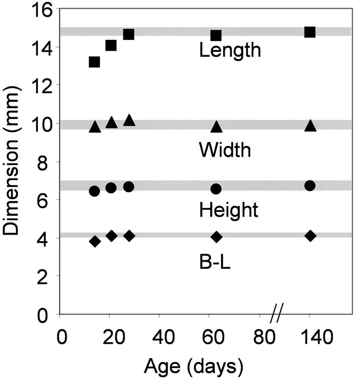
Changes in skull dimensions of the C57BL/6J mouse during development, from age P14 to adult (P140), from the sample population used in this study. The shaded zones indicate the 95% reliability ranges for the skull length, width, height and B-L length obtained from the adult samples.
The recent CT-based study by Chan et al. (2007) demonstrated consistent differences in skull landmarks between C57BL and 129/Sv mice, indicating probable errors if C57BL atlases are applied to different murine strains. Differences in the volumes of internal neuroanatomical components have recently been documented among BXD recombinant inbred mouse lines, which are of particular value for genetic analysis (Jan et al., 2008; Badea et al., 2009; Rosen et al., 2009). More data are needed to determine how adequate a skull dimension-based correction would be for adult mouse brains of different sizes and strains.
In summary, we have created MRI-CT atlases of developing and adult C57BL/6J mouse brains. The single-subject atlases include P7, P14, P21, P28, P63, and P140 brains. For the adult (P140–P160) brain, population-averaged and deformation-corrected atlases were created. All atlases are accessible with our user-interface software. These resources are designed to improve the accuracy of stereotaxic targeting during surgical operations in the C57BL/6J mouse brain.
Acknowledgments
This study was supported by National Institutes of Health grants RO1EB003543, RO1ES012665, RO1AG20012, and P41RR15241.
Abbreviations
- AVM
anatomical variability magnitude map
- CT
computed tomography
- MRI
magnetic resonance imaging
- DTI
diffusion tensor imaging
- FA
fractional anisotropy
- LDDMM
large deformation diffeomorphic metric mapping
- PBS
phosphate buffered saline
- SNR
signal to noise ratio
Footnotes
Publisher's Disclaimer: This is a PDF file of an unedited manuscript that has been accepted for publication. As a service to our customers we are providing this early version of the manuscript. The manuscript will undergo copyediting, typesetting, and review of the resulting proof before it is published in its final citable form. Please note that during the production process errors may be discovered which could affect the content, and all legal disclaimers that apply to the journal pertain.
References
- Alexander DC, Pierpaoli C, Basser PJ, Gee JC. Spatial transformations of diffusion tensor magnetic resonance images. IEEE Trans Med Imaging. 2001;20(11):1131–1139. doi: 10.1109/42.963816. [DOI] [PubMed] [Google Scholar]
- Ali AA, Dale AM, Badea A, Johnson GA. Automated segmentation of neuroanatomical structures in multispectral MR microscopy of the mouse brain. NeuroImage. 2005;27:425–435. doi: 10.1016/j.neuroimage.2005.04.017. [DOI] [PubMed] [Google Scholar]
- Allen Mouse Brain Atlas [Internet]: Allen Institute for Brain Science. http://mouse.brain-map.org.
- Athos J, Storm D. High precision stereotaxic surgery in mice. Current Protocols in Neuroscience Appendix. 2001;4A:1–9. doi: 10.1002/0471142301.nsa04as14. [DOI] [PubMed] [Google Scholar]
- Badea A, Ali-Sharief AA, Johnson GA. Morphometric analysis of the C57BL/6J mouse brain. NeuroImage. 2007;37(3):683–693. doi: 10.1016/j.neuroimage.2007.05.046. [DOI] [PMC free article] [PubMed] [Google Scholar]
- Badea A, Johnson GA, Williams RW. Genetic dissection of the mouse brain using high-field magnetic resonance microscopy. NeuroImage. 2009 doi: 10.1016/j.neuroimage.2009.01.021. [DOI] [PMC free article] [PubMed] [Google Scholar]
- Baldock R, Bard J, Brune R, Hill B, Kaufman M, Opstad K, Smith D, Stark M, Waterhouse A, Yang Y, Davidson D. The Edinburgh mouse atlas: using the CD. Brief Bioinform. 2001;2:159–169. doi: 10.1093/bib/2.2.159. [DOI] [PubMed] [Google Scholar]
- Baloch S, Verma R, Huang H, Khurd P, Clark S, Yarowsky P, Abel T, Mori S, Davatzikos C. Quantification of brain maturation and growth patterns in C57BL/6J mice via computational neuroanatomy of diffusion tensor images. Cereb Cortex. 2009;19(3):675–687. doi: 10.1093/cercor/bhn112. [DOI] [PMC free article] [PubMed] [Google Scholar]
- Barbarese E, Carson J, Braun P. Accumulation of the four myelin basic proteins in mouse brain during development. J Neurochem. 1978;31(4):779–782. doi: 10.1111/j.1471-4159.1978.tb00110.x. [DOI] [PubMed] [Google Scholar]
- Basser PJ, Mattiello J, LeBihan D. Estimation of the effective self-diffusion tensor from the NMR spin echo. J Magn Reson B. 1994;103:247–254. doi: 10.1006/jmrb.1994.1037. [DOI] [PubMed] [Google Scholar]
- Benveniste H, Kim K, Zhang L, Johnson G. Magnetic resonance microscopy of the C57BL mouse brain. NeuroImage. 2000;11:601–611. doi: 10.1006/nimg.2000.0567. [DOI] [PubMed] [Google Scholar]
- Bock NA, Kovacevic N, Lipina TV, Roder JC, Ackerman SL, Henkelman RM. In vivo magnetic resonance imaging and semiautomated image analysis extend the brain phenotype for cdf/cdf mice. J Neurosci. 2006;26(17):4455–4459. doi: 10.1523/JNEUROSCI.5438-05.2006. [DOI] [PMC free article] [PubMed] [Google Scholar]
- Carson J, Nielson M, Barbarese E. Developmental regulation of myelin basic protein expression in mouse brain. Dev Biol. 1983;96(2):485–492. doi: 10.1016/0012-1606(83)90185-9. [DOI] [PubMed] [Google Scholar]
- Chahboune H, Ment LR, Stewart WB, Ma X, Rothman DL, Hyder F. Neurodevelopment of C57B/L6 mouse brain assessed by in vivo diffusion tensor imaging. NMR Biomed. 2007;20(3):375–382. doi: 10.1002/nbm.1130. [DOI] [PubMed] [Google Scholar]
- Chan E, Kovacevic N, Ho SK, Henkelman RM, Henderson JT. Development of a high resolution three-dimensional surgical atlas of the murine head for strains 129S1/SvImJ and C57Bl/6J using magnetic resonance imaging and micro-computed tomography. Neuroscience. 2007;144(2):604–615. doi: 10.1016/j.neuroscience.2006.08.080. [DOI] [PubMed] [Google Scholar]
- Dhenain M, Ruffins SW, Jacobs RE. Three-dimensional digital mouse atlas using high-resolution MRI. Dev Biol. 2001;232(2):458–470. doi: 10.1006/dbio.2001.0189. [DOI] [PubMed] [Google Scholar]
- Dong HW. The Allen Reference Atlas: A Digital Color Brain Atlas of the C57BL/6J Male Mouse (DVD Edition) New York: Wiley; 2008. [Google Scholar]
- Dorr AE, Lerch JP, Spring S, Kabani N, Henkelman RM. High resolution three-dimensional brain atlas using an average magnetic resonance image of 40 adult C57Bl/6J mice. NeuroImage. 2008;42(1):60–69. doi: 10.1016/j.neuroimage.2008.03.037. [DOI] [PubMed] [Google Scholar]
- Franklin KBL, Paxinos G. The Mouse Brain in Stereotaxic Coordinates. 1. San Diego: Academic Press; 1997. [Google Scholar]
- Franklin KBJ, Paxinos G. The Mouse Brain in Stereotaxic Coordinates. 3. New York: Elsevier; 2008. [Google Scholar]
- Hof PR, Young WG, Bloom FE, Belichenko PV, Celio MR. Comparative Cytoarchitectonic Atlas of the C57BL/6 and 129/Sv Mouse Brains. Amsterdam: Elsevier; 2000. [Google Scholar]
- Jacobowitz DM, Abbott LC. Chemoarchitectonic atlas of the developing mouse brain. CRC; 1997. [Google Scholar]
- Jacobs RE, Ahrens ET, Dickinson ME, Laidlaw DH. Towards a microMRI atlas of mouse development. Comput Med Imaging Graph. 1999;23(1):15–24. doi: 10.1016/s0895-6111(98)00059-7. [DOI] [PubMed] [Google Scholar]
- Jan T, Lu L, Li C, Williams RW, Waters R. Genetic analysis of posterior medial barrel subfield (PMBSF) size in somatosensory cortex (SI) in recombinant inbred strains of mice. BMC Neurosci. 2008;9:3. doi: 10.1186/1471-2202-9-3. [DOI] [PMC free article] [PubMed] [Google Scholar]
- Kaufman M. Atlas of Mouse Brain Development. London: Academic Press; 1992. [Google Scholar]
- Kovacevic N, Henderson JT, Chan E, Lifshitz N, Bishop J, Evans AC, Henkelman RM, Chen XJ. A three-dimensional atlas of the mouse brain with estimates of the average and variability. Cereb Cortex. 2005;15(5):639–645. doi: 10.1093/cercor/bhh165. [DOI] [PubMed] [Google Scholar]
- Kretschmann HJ, Weinrich W. Neurofunctional systems: 3D reconstructions with correlated neuroimaging. Thieme Medical Publishers; 1997. [Google Scholar]
- Kruger L, Saporta S, Swanson L. Photographic Atlas of the Rat Brain: The Cell and Fiber Architecture Illustrated in Three Planes with Stereotaxic Coordinates. Cambridge: Cambridge University Press; 1995. [Google Scholar]
- Larvaron P, Boespflug-Tanguy O, Renou J, Bonny J. In vivo analysis of the post-natal development of normal mouse brain by DTI. NMR Biomed. 2007;20(4):413–421. doi: 10.1002/nbm.1082. [DOI] [PubMed] [Google Scholar]
- Lee EF, Jacobs RE, Dinov I, Leow A, Toga AW. Standard atlas space for C57BL/6J neonatal mouse brain. Anat Embryol (Berl) 2005;210(4):245–263. doi: 10.1007/s00429-005-0048-y. [DOI] [PubMed] [Google Scholar]
- Lein ES, Hawrylycz MJ, Ao N, Ayres M, Bensinger A, Bernard A, Boe AF, Boguski MS, Brockway KS, Byrnes EJ, Chen L, Chen L, Chen TM, Chin MC, Chong J, Crook BE, et al. Genome-wide atlas of gene expression in the adult mouse brain. Nature. 2007;445:168–176. doi: 10.1038/nature05453. [DOI] [PubMed] [Google Scholar]
- Ma Y, Hof PR, Grant SC, Blackband SJ, Bennett R, Slatest L, McGuigan M, Benveniste H. A three-dimensional digital atlas database of the adult C57BL/6J mouse brain by magnetic resonance microscopy. Neuroscience. 2005;135(4):1203–1215. doi: 10.1016/j.neuroscience.2005.07.014. [DOI] [PubMed] [Google Scholar]
- Ma Y, Smith D, Hof PR, Foerster B, Hamilton S, Blackband SJ, Yu M, Benveniste H. In vivo 3D digital atlas of the adult C57BL/6J mouse brain by magnetic resonance microscopy. Front Neuroanat. 2008;2:1. doi: 10.3389/neuro.05.001.2008. [DOI] [PMC free article] [PubMed] [Google Scholar]
- MacKenzie-Graham A, Lee EF, Dinov ID, Bota M, Shattuck DW, Ruffins S, Yuan H, Konstantinidis F, Pitiot A, Ding Y, Hu G, Jacobs RE, Toga AW. A multimodal, multidimensional atlas of the C57BL/6J mouse brain. J Anat. 2004;204(2):93–102. doi: 10.1111/j.1469-7580.2004.00264.x. [DOI] [PMC free article] [PubMed] [Google Scholar]
- Miller MI, Trouve A, Younes L. On the metrics and euler-lagrange equations of computational anatomy. Annu Rev Biomed Eng. 2002;4:375–405. doi: 10.1146/annurev.bioeng.4.092101.125733. [DOI] [PubMed] [Google Scholar]
- Mori S, Itoh R, Zhang J, Kaufmann WE, van Zijl PCM, Solaiyappan M, Yarowsky P. Diffusion tensor imaging of the developing mouse brain. Magn Reson Med. 2001;46:18–23. doi: 10.1002/mrm.1155. [DOI] [PubMed] [Google Scholar]
- Mori S, van Zijl PCM. A motion correction scheme by twin-echo navigation for diffusion weighted magnetic resonance imaging with multiple RF echo acquisition. Magn Reson Med. 1998;40:511–516. doi: 10.1002/mrm.1910400403. [DOI] [PubMed] [Google Scholar]
- Paxinos G, Halliday G, Watson C, Koutcherov Y, Wang H. Atlas of the developing mouse brain at E17.5, P0, and P6. San Diego: Elsevier; 2007. [Google Scholar]
- Paxinos G, Watson C. The rat brain in stereotaxic coordinates. 1. Sydney: Academic Press; 1982. [DOI] [PubMed] [Google Scholar]
- Pellegrino LJ, Pellegrino AS, Cushman AJ. A Stereotaxic Atlas of the Rat Brain. New York: Plenum Press; 1979. [Google Scholar]
- Petiet AE, Kaufman MH, Goddeeris MM, Brandenburg J, Elmore SA, Johnson GA. High-resolution magnetic resonance histology of the embryonic and neonatal mouse: A 4D atlas and morphologic database. PNAS. 2008;105(34):12331–12336. doi: 10.1073/pnas.0805747105. [DOI] [PMC free article] [PubMed] [Google Scholar]
- Rosen G, Pung C, Owens C, Caplow J, Kim H, Mozhui K, Lu L, Williams RW. Genetic modulation of striatal volume by loci on Chrs 6 and 17 in BXD recombinant inbred mice. Genes Brain Behav. 2009 doi: 10.1111/j.1601-183X.2009.00473.x. [DOI] [PMC free article] [PubMed] [Google Scholar]
- Schambra U. Prenatal Mouse Brain Atlas. New York: Springer-Verlag; 2008. [Google Scholar]
- Schuz A, Chaimow D, Liewald D, Dortenman M. Quantitative aspects of corticocortical connections: A tracer study in the mouse. Cereb Cortex. 2006;16:1474–1486. doi: 10.1093/cercor/bhj085. [DOI] [PubMed] [Google Scholar]
- Sharief A, Badea A, Dale A, Johnson GA. Automated segmentation of the actively stained mouse brain using multi-spectral MR microscopy. NeuroImage. 2008;39(1):136–145. doi: 10.1016/j.neuroimage.2007.08.028. [DOI] [PMC free article] [PubMed] [Google Scholar]
- Sidman RL, Angevine JB, Taber-Pierce E. Atlas of the mouse brain and spinal cord (Commonwealth Fund Publications) Cambridge: Harvard University Press; 1971. [Google Scholar]
- Slotnick B, Leonard C. A Stereotactic Atlas of the Albino Mouse Forebrain. DHEW Publication, Rockville, MD: U. S. Government Printing Office; 1975. [Google Scholar]
- Valverde F. Golgi Atlas of the Postnatal Mouse Brain. New York: Springer-Verlag; 2004. [Google Scholar]
- Verma R, Mori S, Shen D, Yarowsky P, Zhang J, Davatzikos C. Spatiotemporal maturation patterns of murine brain quantified by diffusion tensor MRI and deformation-based morphometry. PNAS. 2005;102(19):6978–6983. doi: 10.1073/pnas.0407828102. [DOI] [PMC free article] [PubMed] [Google Scholar]
- Vincze A, Mazlo M, Seress L, Komoly S, Abraham H. A correlative light and electron microscopic study of postnatal myelination in the murine corpus callosum. Int J Dev Neurosci. 2008;26(6):575–584. doi: 10.1016/j.ijdevneu.2008.05.003. [DOI] [PubMed] [Google Scholar]
- Westin CF, Maier SE, Mamata H, Nabavi A, Jolesz FA, Kikinis R. Processing and visualization for diffusion tensor MRI. Med Image Anal. 2002;6(2):93–108. doi: 10.1016/s1361-8415(02)00053-1. [DOI] [PubMed] [Google Scholar]
- Williams RW. Mapping genes that modulate mouse brain development: a quantitative genetic approach. In: Goffinet AF, Rakic P, editors. Mouse Brain Development. New York: Springer-Verlag; 2000. pp. 21–49. [DOI] [PubMed] [Google Scholar]
- Xu D, Mori S, Shen D, van Zijl PCM, Davatzikos C. Spatial normalization of diffusion tensor fields. Magn Reson Med. 2003;50(1):175–182. doi: 10.1002/mrm.10489. [DOI] [PubMed] [Google Scholar]
- Zhang J, Miller MI, Plachez C, Richards LJ, Yarowsky P, Van Zijl PCM, Mori S. Mapping postnatal mouse brain development with diffusion tensor microimaging. NeuroImage. 2005;26(4):1042–1051. doi: 10.1016/j.neuroimage.2005.03.009. [DOI] [PubMed] [Google Scholar]
- Zhang W, Li X, Zhang J, Luft A, Hanley DF, Van Zijl PCM, Miller MI, Younes L, Mori S. Landmark-referenced voxel-based analysis of diffusion tensor images of the brainstem white matter tracts: Application in patients with middle cerebral artery stroke. NeuroImage. 2009;44(3):906–913. doi: 10.1016/j.neuroimage.2008.09.013. [DOI] [PMC free article] [PubMed] [Google Scholar]
- Zimmermann B, Moegelin A, de Souza P, Bier J. Morphology of the development of the sagittal suture of mice. Anat Embryol. 1998;197:155–165. doi: 10.1007/s004290050127. [DOI] [PubMed] [Google Scholar]