A stochastic neighborhood conditional autoregressive model for spatial data

Abstract

A spatial process observed over a lattice or a set of irregular regions is usually modeled using a conditionally autoregressive (CAR) model. The neighborhoods within a CAR model are generally formed deterministically using the inter-distances or boundaries between the regions. An extension of CAR model is proposed in this article where the selection of the neighborhood depends on unknown parameter(s). This extension is called a Stochastic Neighborhood CAR (SNCAR) model. The resulting model shows flexibility in accurately estimating covariance structures for data generated from a variety of spatial covariance models. Specific examples are illustrated using data generated from some common spatial covariance functions as well as real data concerning radioactive contamination of the soil in Switzerland after the Chernobyl accident.

1. Introduction

The accident that occurred at the Chernobyl nuclear power plant on April 26, 1986 was one of the most serious nuclear power plant catastrophes in history. Discharge from the plant lasted for ten days and deposited a variety of radioactive particles into the atmosphere. Predicting and monitoring the pattern of contamination across Europe has been difficult, due to the variety of radioactive particles, as well as the meteorological conditions. In the ensuing period data on contamination has been collected across Europe. We analyze a subset of this data collected at 200 irregularly located sites across Switzerland. This data consists of observations of cesium (¹³⁷Cs) concentration per square meter measured in kBq/m² where 1 Bq = one radioactive decay per second (Kanevski and Maignan, 2004). This concentration is of interest because it is thought to be a good overall indicator of contamination levels.

Data of this type can be modeled using either a traditional geostatistical model where the spatial dependence between observed concentrations is captured based on estimating parameters of a weakly stationary isotropic covariance function. The covariance is defined as a function of some measure of the separation between observations' locations. Commonly used covariance weakly stationary functions are Exponential, Gaussian or more generally the Matern family (Cressie, 1993). However, the use of such stationary isotropic covariance models may not be appropriate for our motivation data set as we shall show in Section 4. Alternatively, a conditionally autoregressive (CAR) model can also be used. In the CAR model spatial dependence is expressed through the mean term by setting the expected value of observations in a region to be a function of the adjacent areas' means (Besag, 1974). Traditionally geostatistical models are considered more flexible in capturing the spatial dependence when a large number of observations can be measured at different sites. The disadvantage to these models is in the computational burden involved as well as the limitation of the available models for non-stationary covariance structures. CAR models are seen typically as too restrictive in the range of spatial dependence that they will model successfully, though computationally they offer an advantage over geostatistical models (Rue and Tjelmeland, 2002).

Due to potential non-standard features in the data such as anisotropy or non-stationarity it is desirable to perform an analysis using a class of spatial models that are as flexible as possible. The size of the dataset studied here, though not excessive lends itself to any effort to improve computational efficiency, as is useful in general for spatial data analysis. In order to accomplish these goals we extend the family of Gaussian–Markov Random Fields (MRF) proposed by Hrafnkelesson and Cressie (2003) for the regular lattice to the case of an irregular lattice and allow for a stochastic variation of neighborhood for a CAR model. This model combines the flexibility of a geostatistical model with the computational advantages of a CAR model. The resulting model demonstrates good characteristics for fitting data from a variety of spatial covariance models. In addition it is also computationally efficient and easy to implement for large data sets.

In Section 2, we discuss some of the existing models and present our extension. In Section 3, we present results based on measuring the Kullback–Liebler discrepancies between true data generating distribution and the proposed model. We also use simulated data sets to compare the performance of our proposed model to other existing models. In Section 4, we apply our proposed model to the motivating data of cesium-137 (¹³⁷Cs) contamination in Switzerland and discuss the results. Finally we close with a discussion of the overall results and directions for possible future work in Section 5.

2. Spatial models

Spatial data can be defined as observed over either specific sites or areas. In the first case, analysis involves using a geostatistical model where the covariance is defined as a function of some measure of the separation between the location of observations (Cressie, 1993). In the case of areal data covariance is modeled typically as a function of the adjacency structure of the areas, as in a CAR model, or in general as a Markov Random Field on a regular discrete lattice. For point referenced data the observations are made on a continuous spatial region, rather than a discrete grid. It has been demonstrated that the difference between these two approaches is not as distinct as it may initially appear (Werner, 2004; Song et al., in press). We demonstrate that the proposed Stochastic Neighborhood CAR (SNCAR) model can better approximate some of the common geostatistical models as compared to regular CAR models.

In our application ¹³⁷Cs concentration was measured at 200 sites. The locations of these sites are irregularly located and are most likely not randomly selected. It is assumed that the concentrations are highly correlated in space. This motivated the use of a spatial model. The use of an MRF model is motivated by the desire to improve computational efficiency and to explore the capabilities of anisotropy and non-stationarity in the proposed model.

2.1. Gaussian MRFs

We begin the development of our model by reviewing the definition of a Gaussian Markov Random Field. For y = (y(s₁), …, y(s_n))′ an n×1 vector of observations at locations {s₁, …, s_n} from a spatial process the full conditional means and variances can be written as

$$E(y\left({\mathit{s}}_i\right)\mid \{y\left({\mathit{s}}_j\right):j\ne i\})={\mu }_i+\rho \underset{j=1}{\overset{n}{\Sigma }}{c}_{\mathit{ij}}\{y\left({\mathit{s}}_j\right)-{\mu }_j\}∕\underset{j=1}{\overset{n}{\Sigma }}{c}_{\mathit{ij}}$$ (1)

and

$$\mathrm{Var}(y\left({\mathit{s}}_i\right)\mid \{y\left({\mathit{s}}_j\right):j\ne i\})={\sigma }^2∕\underset{j=1}{\overset{n}{\Sigma }}{c}_{\mathit{ij}}.$$ (2)

If we assume that each of these univariate full conditional distributions are normally distributed then it follows from Brook's Lemma (Besag, 1974) that the joint distribution is an n-dimensional multivariate normal distribution given by

$$\mathit{y}\sim N(\mu ,{\sigma }^2{(\mathit{D}-\rho \mathit{C})}^{-1}),$$ (3)

where ρ is a parameter describing the relative strength of spatial dependence, C is an n × n matrix such that c_ij = c_ji and c_ii = 0, and D is a diagonal matrix with diagonal entries $d_{\mathit{ii}}={\Sigma }_{j=1}^n{c}_{\mathit{ij}}$. This form is most familiar as a CAR model, where C is commonly chosen as the adjacency matrix with c_ij = 1 if areas i and j are adjacent and 0 otherwise (Besag and Kooperberg, 1995). In general this form is not strictly limited to the traditional CAR model definition of adjacency in defining C. The matrix C can be defined in a variety of ways as long as the resulting matrix, (D − ρC) is positive definite (Banerjee et al., 2004) for a range of parameter values and any number of sites/regions. As a result we define C using a similar neighborhood measure proposed by Hrafnkelesson and Cressie (2003) for a Markov random field. The resulting model can be used as an approximation of the geostatistical model over a continuous spatial index, as the regions shrink to their centroids.

2.2. The SNCAR model

In this section we propose a neighborhood measure that defines the off diagonal elements of the matrix C which are allowed to change with unknown parameter(s). A neighborhood function can be defined in several different ways as long as the resulting matrix C is symmetric and (D − ρC) is positive definite. In particular when the observations are point referenced, it is desirable to create a neighborhood measure based on d_ij, the intra-point distance for pairs of locations or centroid of a pair of regions. In the case of data on a regular lattice the adjacency function for a CAR model, given an upper limit d_u is c_ij = I(0 < d_ij ≤ d_u) where I(·) denotes the indicator function taking the value 1 if the condition within (·) is satisfied and taking the value 0 otherwise. For areal data the definition is

$$c_{\mathit{ij}}=\{\begin{array}{cc}1\hfill & \text{if regions}i\text{and}j\text{share a common boundary for}i\ne j\hfill \\ 0\hfill & \text{otherwise}.\hfill \end{array}\phantom{\}}$$ (4)

If the observed areas are on a regular lattice (4) is the same as c_ij = I(0 < d_ij ≤ d_u) where d_u is the largest distance between the centroid for locations that are considered adjacent. For an irregular lattice, d_u is chosen such that no row of C will have all 0 entries. Other choices are also available for defining d_u, though caution should be exercised to maintain the positive definiteness of the matrix D − ρC. The result is a step function which coincides with the CAR adjacency matrix definition of the neighborhood measure for regular grids. In general this neighborhood function can be defined as

$$c_{\mathit{ij}}=\{\begin{array}{cc}1\hfill & \text{if}0<d_{\mathit{ij}}\le d_l,\hfill \\ c(d_{\mathit{ij}},\psi )\hfill & \text{if}{d}_l<d_{\mathit{ij}}<d_u,\hfill \\ 0\hfill & \text{otherwise},\hfill \end{array}\phantom{\}}$$ (5)

where c(d_ij,ψ) is some function such that c(d_ij,ψ) ≤ 1, which may depend on unknown parameters ψ. As in Hrafnkelesson and Cressie (2003), we employ the following function $c(d_{\mathit{ij}},\psi )=d_{\mathit{ij}}^{-\psi }$ where ψ = −log(α)/log(d_u) and α > 0 is the amount of spatial dependence present when d_ij is equal to some upper limit d_u; in this paper we set α = 0.05. The value d_l is chosen to ensure that the resulting matrix D − ρC(ψ) is positive definite, and d_u is chosen as an unknown upper limit for adjacency to be estimated. The parameter d_u helps us to ensure that the resulting precision matrix D − ρC(ψ) is sparse, and d_l ensures that it is not too sparse. Note that d_ij can always be scaled such that the smallest non-zero value of d_ij, d_l = 1 so that c(d_ij,ψ) is strictly decreasing in d_ij, for i ≠ j. The resulting spatial model has the form of a traditional CAR model and if the parameter ψ is considered a random variable then the resulting model is a stochastic neighborhood conditional autoregressive (SNCAR) model.

3. Performance of SNCAR model

In order to compare the performance of a given spatial model we use the Kullback–Liebler discrepancy (KLD) of the proposed model to the true data generating distribution. Suppose that data y is generated from a density f(y|A₀) and the proposed model is based on f(y|A), where A₀ and A denote the precision matrices under the true and proposed models, respectively. If we assume that our data are generated from zero mean Gaussian distributions, then it easily follows that −2 logf(y|A_j) = n log(2π) + y_TA_jy − log(|A_j|) for j = 0, 1 and hence the KLD between f(y|A₀) and f(y|A) is given by

$$\begin{array}{cc}\hfill D(\mathit{A}\mid {\mathit{A}}_0)& =\int f(\mathit{y}\mid {\mathit{A}}_0)\log \left(\frac{f(\mathit{y}\mid {\mathit{A}}_0)}{f(\mathit{y}\mid \mathit{A})}\right)\mathrm{d}\mathit{y}\hfill \\ \hfill & =\frac{1}{2}[\mathrm{tr}\left({\mathit{AA}}_0^{-1}\right)-\log \mid {\mathit{AA}}_0^{-1}\mid -n].\hfill \end{array}$$

Now given a true precision matrix A₀ and two competing models with precision matrices A₁ and A₂ we can find Â₁ and Â₂ that minimize D(A₁|A₀) and D(A₂|A₀), respectively. The model with precision matrix A₁ is said to perform better than the model with precision matrix A₂ if D(Â₁|A₀) < D(Â₂|A₀). Next we consider several choices for the true precision matrix A₀ and compare the performance of the SNCAR with another competing model. For all our illustrations we use the centroid of the counties in Missouri as our choice for the sites s₁, …, s_n. The main difference between the hierarchical models for the CAR, exponential and SNCAR models is in the spatial covariance (or equivalently the precision) matrix used and the associated priors.

(a) The CAR model

The hierarchical model is specified as

$$\begin{array}{cc}\hfill & \mathit{y}\mid {\delta }_0,\rho \sim N(0,{\delta }_0{(\mathit{D}-\rho \mathit{C})}^{-1}),\hfill \\ \hfill & {\delta }_0\sim \text{InvGamma}(a_0=0.1,b_0=0.1),\hfill \end{array}$$

and

$$\rho \sim \text{Beta}(2,1).$$

For the example here we have an adjacency matrix for Missouri based on (4). When the CAR model is chosen as the data generating distribution we used ρ = (0.2, 0.5, 0.9) and δ₀ = (0.1, 1, 10) which results into nine different CAR models. Notice that the CAR precision matrix is given by A(δ₀, ρ) = (D − ρC)/δ₀.

(b) The Exponential model:

The hierarchical model is specified as

$$\begin{array}{cc}\hfill & \mathit{y}\mid {\delta }_0,\varphi \sim N(0,\Sigma ({\delta }_0,\varphi )),\text{where}{\sigma }_{\mathit{ij}}={\delta }_0\exp (-\varphi d_{\mathit{ij}}),\hfill \\ \hfill & \varphi \sim U(0.01,41),\hfill \end{array}$$

and

$${\delta }_0\sim \text{InvGamma}(a_0=0.1,b_0=0.1).$$

The range (0.01, 41) for the uniform prior on ϕ is chosen based on prior beliefs about the maximum and minimum correlation at the largest and smallest distances of the data. When the Exponential model is chosen as the true data generating distribution we used ϕ = (3, 0.31, 0.17) and δ₀ = (0.1, 1, 10) resulting into nine different true Exponential models. Notice that the Exponential precision matrix is given by A(δ₀, ϕ) = Σ(δ₀, ϕ)⁻¹.

(c) The SNCAR model:

The hierarchical model is specified as

$$\begin{array}{cc}\hfill & \mathit{y}\mid {\delta }_0,\rho ,\Delta \sim N(0,{\delta }_0{(\mathit{D}-\rho \mathit{C}\left(\psi \right))}^{-1}),\hfill \\ \hfill & {\delta }_0\sim \text{InvGamma}(a_0=0.1,b_0=0.1),\hfill \\ \hfill & \Delta \sim \text{Uniform}(d_l+∊,10)\text{where}\Delta =d_u-d_l,\hfill \\ \hfill & \rho \sim \text{Beta}(2,1)\hfill \end{array}$$

and

$$\psi =-\log \left(\alpha \right)∕\log (d_l+\Delta )$$

where d_l is fixed at a suitable value so that the resulting precision matrix is positive definite and ψ = −log(α)/ log(d_u) with α = 0.05. The prior for Δ is chosen with ∊ = 0.0001 and the upper limit reflecting a reasonable belief about the maximum distance, in this case this upper limit is approximately 1/3 the maximum distance between centroid. Notice that the SNCAR precision matrix is given by A(δ₀, ρ, ψ) = (D – ρC(ψ))/δ₀ where ψ is a decreasing function of Δ.

3.1. KLD comparison between SNCAR and competing models

We present the performance of the SNCAR when the true data arise either from a given CAR model (as specified in (a)) or a given Exponential model (as specified in (b)). Specifically, suppose A₀ ≡ A₀(δ₀, ρ) to be the precision matrix corresponding a given CAR model, let A₁(δ₀, ρ, ψ) represent the precision matrix of a SNCAR model as defined above. Let A₂(δ₀, ϕ) denote the precision matrix of an exponential covariance model with range ϕ and partial sill δ₀. We use numerical optimization to obtain (ψ̂, σ̂², ρ̂) that minimizes D(A₁(ψ, σ², ρ)|A₀) and similarly obtain (δ̂₀, ϕ̂) that minimizes D(A₂(δ₀, ϕ)|A₀). In Table 1, we report values of D(A₁(ψ̂, σ̂², ρ̂)|A₀) and D(A₂(δ̂₀, ϕ̂)|A₀) when A₀ is chosen as one of the nine CAR models with true values δ₀ = (0.1, 1, 10) and ρ = (0.3, 0.5, .02). We repeat a similar procedure when A₀ is chosen as one of the nine Exponential model with δ₀ = (0.1, 1, 10) and ϕ = (3, 0.31, 0.19) and report the minimized KLD values in Table 2. The minimized KLD indicates that the proposed SNCAR models outperform both CAR and Exponential models when the models are misspecified as Exponential and CAR, respectively. These results indicate that if a maximum likelihood procedure is used, then the proposed SNCAR model would provide a better fit when the true precision matrix is misspecified.

Table 1.

The minimized KLD of the SNCAR (A₁) and exponential (A₂) models relative to true CAR (A₀) model

δ0	ρ	SNCAR	Exp	ρ	SNCAR	Exp	ρ	SNCAR	Exp
0.1	0.3	60.42	64.33	0.5	61.53	66.47	0.9	67.83	74.66
1.0	0.3	60.41	64.33	0.5	61.53	66.47	0.9	65.50	74.66
10.0	0.3	58.97	64.33	0.5	59.32	66.47	0.9	60.62	74.66

Table 2.

The minimized KLD of the SNCAR (A₁) and CAR (A₂) models relative to true exponential (A₀) model

δ0	ϕ	SNCAR	CAR	ϕ	SNCAR	CAR	ϕ	SNCAR	CAR
0.1	3	59.28	60.28	0.37	60.63	62.91	0.19	61.60	64.73
1.0	3	59.29	60.28	0.37	60.54	62.91	0.19	61.59	64.73
10.0	3	59.40	60.28	0.37	60.54	62.91	0.19	61.64	64.73

3.2. Simulation study to compare the out-of-sample performance of the SNCAR model

Next in order to asses the predictive performance of the SNCAR model as compared to the Exponential and CAR models we use data sets simulated from Exponential and CAR models. For each of the previously stated covariance matrices (see (a) and (b) in Section 3) ten data sets of size 115 are generated from each of nine CAR and nine Exponential models as the true models. Thus, we have eighteen true models with ten replicated data sets for each. For each of the 180 data sets we fit a CAR, Exponential and SNCAR models with priors as specified in (a)–(c) and obtain posterior samples. For each of the 90 data sets generated from a CAR (or Exponential) model, a random subset of 15 observations is withheld and their values are predicted using the posterior predictive distribution under the assumed model. If y^w denotes the vector of 15 withheld values and if y^pred denotes the corresponding vector of 15 predicted values, we measure the predictive performance by the sum of squared predictive errors (SSPE) given by SSPE = ||y^pred – y^w||², where || · || denotes the Euclidean norm. Notice that, if y^obs denote the vector of observed 100 values that were used to fit the model then MSPE = E[SSPE|y^obs] = tr(V^w)+||μ^w–y^w||², where V^w = Var[y^pred|y^obs] and μ^w = E[y^pred|y^obs] denote the predicitve variance and the mean of y^pred given y^obs, respectively. Notice that as the data sets are generated from zero mean Gaussian distributions, both μ^w and y^w are expected to be close to zero vector and hence the dominating term of MSPE would be the tr(V^w), where tr(·) denotes the trace of the matrix. Thus, the predictive performance of the models is in their ability to predict the covariance structure of the withheld data. The difference is then entirely in the estimation of the covariance matrices. In this predictive measure, it is easy to see that the SNCAR model outperforms the other models for the misspecified data.

3.3. Performance of SNCAR based on comparing DIC

In addition to the predictive sum of squares and trace metric used to compare models under misspecification we also calculated DIC and p_D (Spiegelhalter et al., 2002) for each of the ten replicates of the eighteen different models fit. The results are shown in Tables 5 and 6 and Figs. 4-9 (see Appendix). It is clearly evident that when the true model is a CAR and we fit SNCAR and EXP models, the SNCAR provides a much better fit (in terms having lower DIC), in comparison to the EXP model for all possible eighteen combinations of the parameter values. In Table 5 we see by comparing the p_D values, that the SNCAR model uses effectively more parameters compared to the EXP model but in terms of DIC values the SNCAR model is preferred, as evidenced by the lower DIC. Also from Table 6 it appears that in most cases SNCAR is preferable to the CAR model when the data is generated from the EXP model. Except for two cases when ϕ = 3 and δ₀ = 0.1 and 1. In these two cases the spatial correlation is rather weak (recall that σ_ij = δ₀ exp(−ϕd_ij)) and the observations are nearly white noise. In all other scenarios, especially when the true spatial autocorrelation is comparatively strong, the SNCAR outperforms the other two commonly used models in terms of DIC and the other two measures that we described in the earlier two subsections.

Table 5.

The mean DIC and (p_D) of the SNCAR (A₁) and exponential (A₂) models relative to true CAR (A₀) model

δ0	ρ	SNCAR	Exp	ρ	SNCAR	Exp	ρ	SNCAR	Exp
0.1	0.3	10007 (538.74)	11218 (69.187)	0.5	9279.1 (443.67)	9926.7 (539.07)	0.9	7679.6 (382.29)	8454.8 (2166.2)
1.0	0.3	1199.9 (54.199)	1224.7 (10.768)	0.5	1301.9 (62.990)	1243.9 (33.142)	0.9	1012.6 (37.521)	1058.0 (220.42)
10.0	0.3	412.29 (5.2382)	417.21 (−1.2766)	0.5	408.91 (4.9308)	418.81 (−1.2590)	0.9	398.97 (2.2100)	417.71 (−9.4061)

Table 6.

The mean DIC and (p_D) of the SNCAR (A₁) and CAR (A₂) models relative to true exponential (A₀) model

δ0	ϕ	SNCAR	CAR	ϕ	SNCAR	CAR	ϕ	SNCAR	CAR
0.1	3	2097.0 (104.92)	1952.9 (62.314)	0.37	2335.4 (95.903)	3130.6 (819.07)	0.19	3175.6 (156.01)	3982.6 (1122.5)
1.0	3	463.33 (11.343)	430.02 (6.0676)	0.37	476.95 (8.1129)	727.32 (158.72)	0.19	651.63 (12.341)	685.33 (135.93)
10.0	3	505.85 (−0.0513)	526.76 (2.1660)	0.37	459.72 (−0.3531)	760.98 (112.39)	0.19	423.48 (0.1875)	567.81 (33.616)

Fig. 4.

Density of log(SSPE) for SNCAR (– – –) and Exponential (—) fit to CAR data.

Fig. 9.

Box Plot of DIC for SNCAR and CAR fit to Exponential data.

The occurrence of negative p_D values in several cases of the SNCAR and the exponential models is a notable event. Negative values for deviance and DIC are not necessarily an indication of possible problems with the model. Negative values for p_D do merit further attention. This subject has been addressed in Spiegelhalter et al. (2002) as well as in several recent papers including Celeux et al. (2006) and Plummer (2006). In summary the causes of negative p_D can be the non-log concavity of the sampling distribution, or a posterior distribution where the mean is a poor estimator. Several remedies for this, and other methods of model selection have been proposed. However we have not explored such remedies in this article.

From our extensive simulation study (consisting of 18 different scenarios with 10 replication each), we can safely conclude that, in most practical cases, the proposed SNCAR model will provide a better fit than the CAR or EXP model when the models are misspecified.

4. Application to the Swiss ¹³⁷Cs soil contamination data

In this section we present analysis of the data set that motivated us to develop the SNCAR model. This data was collected after the Chernobyl Nuclear Reactor accident at 200 locations measuring cesium (¹³⁷Cs) concentration per square meter (see Fig. 2). While the contamination consists of several different radioactive isotopes, the concentration of radioactive cesium is an important indicator of overall contamination. A spatial model of concentration is useful for both prediction of concentration at unobserved locations as well as for inference about the general distribution of contaminants across Switzerland. Before we fit the proposed SNCAR model to this data set we performed some exploratory data analysis to check the validity of the assumptions (e.g., Gaussianity, stationarity and isotropy).

Fig. 2.

Bubbleplot of observed ¹³⁷Cs concentrations along with the estimated concentration.

4.1. Exploratory data analysis

Based on some preliminary analysis we find that log-normal distribution would be a suitable family to model the observed concentrations. Let y_i be the natural logarithm of the observed level of ¹³⁷Cs at site s_i = (s_1i, s_2i), for i = 1, …, n = 200, where s_1i and s_2i denote the latitude and longitude of the ith location. Our preliminary analysis suggests that the following model serves as good approximation for the concentration data:

$$y_i={\beta }_0+{\beta }_1{s}_{1i}+{\beta }_2{s}_{2i}+z_i+e_i,$$ (6)

where measurement errors e_i's are independent of the spatial random effects z_i's and β₀, β₁ and β₂ are regression coefficients of the linear trend. The spatial random effect vector z = (z₁, …, z_n) is modeled using one of the three spatial models discussed earlier in Section 3. It is also assumed that the measurement errors e_i's are independent and identically distributed (iid) with mean 0 and variance δ₁.

Further exploratory data analysis was carried out using the geoR package in R software. This initial spatial analysis suggests that the underlying spatial correlations between the sites are anisotropic. Hence, we transform the observed sites s_i's using the following transform

$${\mathit{s}}_i^{\ast }={\mathit{s}}_i\left(\begin{array}{cc}\hfill \cos \left(\theta \right)\hfill & \hfill -\sin \left(\theta \right)\hfill \\ \hfill \sin \left(\theta \right)\hfill & \hfill \cos \left(\theta \right)\hfill \end{array}\right)\left(\begin{array}{cc}\hfill 1\hfill & \hfill 0\hfill \\ \hfill 0\hfill & \hfill {\eta }^{-1}\hfill \end{array}\right)$$ (7)

and use the modified measure of distance

$$d_{\mathit{ij}}^{\ast }=\sqrt{({\mathit{s}}_i^{\ast }-{\mathit{s}}_j^{\ast }){({\mathit{s}}_i^{\ast }-{\mathit{s}}_j^{\ast })}^{\prime }}.$$ (8)

The parameters θ and η denote the angle and ratio respectively, that describe the anisotropy as defined in Diggle and Ribeiro (2007). For all subsequent analysis we fix the angle (θ) and ratio (η) parameters at the maximum likelihood estimates θ̂ = 0.55 and η̂ = 1.374, obtained using geoR Ribeiro and Diggle (2001). Moreover, for numerical stability we have centered (by mean) and scaled (by standard deviation) the response variables y_i's and also the site variables $s_{i1}^{\ast }$ and $s_{i2}^{\ast }$. Hence we can use the simplified model given by

$$y_i={\beta }_1{s}_{1i}^{\ast }+{\beta }_2{s}_{2i}^{\ast }+z_i+e_i,$$ (9)

where the y's and s*'s have been suitably centered and scaled to achieve ${\Sigma }_i{y}_i={\Sigma }_i{s}_{1i}^{\ast }={\Sigma }_i{s}_{2i}^{\ast }=0$ and ${\Sigma }_i{y}_i^2=n-1$. Notice that the intercept is now dropped from the model as its estimate would be essentially zero by using centered responses and predictors.

4.2. Results based on spatial analysis of Swiss data

We estimated the parameters of the model (9) with z distributed as one of the spatial models (a)–(c) as described in Section 3. In addition we also fitted a model without the spatial effect (i.e., setting z_i = 0 in model (9)). In order to compare the four models first we use DIC (Spiegelhalter et al., 2002). The DIC and p_D values are presented in Table 7. Clearly the null model having no spatial effects performs poorly and can be safely eliminated from further considerations. Among the remaining three spatial models SNCAR has the lowest DIC value along with the lowest p_D value. This indicates that the proposed SNCAR model not only provides a better fit to the data but it also used effectively fewer parameters. The SNCAR model did take a longer time than the other two models to converge satisfactorily and was run for 50,000 iterations of burn-in, thereafter retaining 10,000 iterations for posterior inference. This model will be the one discussed in the remainder of this section.

Table 7.

DIC and p_D for various models based on Swiss ¹³⁷Cs data

Model	DIC	pD
Null	690.232	2.021
CAR	−7.594	158.814
Exponential	−272.257	165.199
SNCAR	−300.086	158.610

4.3. Parameter estimates based on the SNCAR model

In this section we present the analysis based on the proposed SNCAR model. The estimates of the various model parameters are of interest in examining the results and better understanding the model. The posterior distributions of the model parameters are summarized in Table 8 and Fig. 1.

Table 8.

Posterior estimates of parameters from SNCAR model

Parameter	Mean	Std. dev.	2.5%	Median	97.5%
δ1	0.007	0.002	0.004	0.007	0.011
δ0	0.024	0.014	0.009	0.015	0.05
ρ	0.994	0.005	0.983	0.996	0.999
Δ	0.505	0.225	0.158	0.384	0.815
β1	0.576	0.091	0.412	0.573	0.797
β2	−0.238	0.056	−0.341	−0.245	−0.113

Fig. 1.

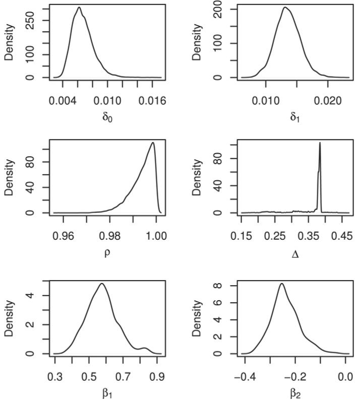
Posterior density estimates of the parameters of SNCAR model fitted to ¹³⁷Cs concentration data.

The density of ρ (in Fig. 1) is extremely skewed to the right (near unity) indicating the presence of a strong spatial effect. The posterior densities (presented in Fig. 1) for δ₀, β₁, and β₂ appear reasonably smooth and unimodal. The posterior estimates of β₁ and β₂ in Table 8 indicate that there is a significant linear trend with concentrations increasing in the southeastern direction and that this trend is statistically significant. There is some roughness in the density estimates for Δ. The posterior correlation between the β's is 0.44 and the posterior correlation between Δ and δ1 is 0.68. This is also possibly the cause of some variance inflation of the parameter estimates as well as inflating the p_D value. All the posterior estimates are based on 10,000 MCMC samples following 50,000 burn-ins obtained via WinBUGS (Lunn et al., 2000).

4.4. Mapping concentrations

In order to evaluate the model performance we employed several graphical plots. In Fig. 2, we present the bubble plot of the observed concentrations and also the estimated concentrations using the posterior predictive mean of the concentration. There appears to be a reasonable similarity between the observed and predicted concentrations. Next to explore the uncertainty of our predicted values we also present the standard errors of the predicted concentrations in Fig. 3 as well as the coefficient of variation. The coefficient of variation (cv) is defined as

$${\mathrm{cv}}_i=\frac{\mathit{sd}(y_i\mid {\mathit{y}}^{\mathrm{obs}})}{E(y_i\mid {\mathit{y}}^{\mathrm{obs}})},$$ (10)

where sd(y_i|y^obs) is the predictive standard error for the estimated concentration E(y_i|y^obs). Smaller values for the cv are more desirable and the value of the cv > 0.3 are considered unreliable (Mendenhall and Sincich, 2003).

Fig. 3.

Standard errors and coefficients of variation of the log-concentrations.

The bubble plot of the observed data and heatmap of the estimated concentrations show that there is one region in the southeast corner that appears to have much higher concentrations than the rest of the area. There is also little smoothing of the data by the model, as evidenced by both the heatmap and the large p_D. This may be due to this prominent anomaly. The large p_D value and the lack of smoothing typically indicate large prediction intervals that compromise the models' predictive ability, and possibly the inferential value of the model as well.

The second set of heatmaps in Fig. 3 shows the standard errors of the estimated concentrations and the coefficients of variation as well. The heatmap of the standard errors indicates that the errors are largest in the regions surrounding the area of lower concentration and are smallest in the areas of highest concentration. This is also expected as we have used a log-normal model which allows the variance to vary with the mean. The heatmap of the cv values shows again that they are lowest in the region of highest concentration, and they are smallest in the region of lowest concentration immediately adjacent. The model in short works best at estimating higher concentrations, which would be of primary interest in assessing health risks. One reason for this result is that the locations where the concentrations are considered low also have a low density of sites. This lack of information and sparseness of locations provide little information for estimating a concentration at a specific site other than the single observation taken there. Another source of variability could be measurement error when observing small values.

The results show that there appears to be an area in south-eastern Switzerland where the concentration of ¹³⁷Cs is higher than that in other areas. Geography may play a role in this as this portion of Switzerland is separated by the Alps mountain range. Since the primary transport mechanism for ¹³⁷Cs is by wind patterns, geographic features such as mountain ranges are an important consideration in interpreting the data. This may also account for the relatively large p_D of the model and the heavy tailed posterior density of Δ.

5. Conclusions

The model results show a good overall fit to the data with standard errors for the fitted values very reasonable. The overall performance of the SNCAR model based on simulated data as well as the analysis of the ¹³⁷Cs data show that it is more flexible in fitting various spatial data. The SNCAR model has the flexibility of traditional geostatistical models while retaining the computational advantages of a CAR model.

The region of higher concentration for the ¹³⁷Cs data may indicate non-stationarity resulting from geographic and meteorological factors. This is a possible cause of the heavy tailed posterior density for Δ. The overall results for the model were good and provide useful information in assessing the underlying ¹³⁷Cs exposure in Switzerland. Incorporation of other predictors, such as altitude, wind speed etc. might improve the model fit.

In this paper we have explained a simple function for c(d_ij, ψ) as defined in (5). It would be of interest to extend the scope of this function to estimate more complicated forms of the neighborhood function. However in making such extensions cautions should be exercised so as to keep the precision matrix positive definite. Our proposed SNCAR can also be used as a prior within the generalized linear model (GLM) by using a suitable link function.

Fig. 5.

Density of log (tr(V^w)) for SNCAR (– – –) and Exponential (—) fit to CAR data.

Fig. 6.

Density of log(SSPE) for SNCAR (– – –) and CAR (—) fit to Exponential data.

Fig. 7.

Density of log (tr(V^w)) for SNCAR (– – –) and CAR (—) fit to Exponential data.

Fig. 8.

Box Plot of DIC for SNCAR and Exponential fit to CAR data.

Table 3.

The MSPE and (mean tr(V^w)) of the SNCAR (A₁) and exponential (A₂) models relative to true CAR (A₀) model

δ0	ρ	SNCAR	Exp	ρ	SNCAR	Exp	ρ	SNCAR	Exp
0.1	0.3	0.926 (0.531)	1.076 (0.348)	0.5	0.982 (0.560)	1.209 (0.394)	0.9	1.438 (0.755)	4.974 (2.225)
1.0	0.3	4.252 (0.525)	10.26 (3.341)	0.5	4.192 (0.561)	10.272 (3.429)	0.9	7.371 (0.758)	71.63 (34.12)
10.0	0.3	38.25 (0.557)	94.08 (32.69)	0.5	40.28 (0.558)	110.97 (34.95)	0.9	63.99 (0.759)	223.3 (86.70)

Table 4.

The MSPE and (Mean of tr(V^w)) of the SNCAR (A₁) and CAR (A₂) models relative to true exponential (A₀) model

δ0	ϕ	SNCAR	CAR	ϕ	SNCAR	CAR	ϕ	SNCAR	CAR
0.1	3	4.107 (2.195)	22.92 (11.12)	0.37	6.109 (3.578)	13726 (7264)	0.17	7.289 (4.694)	49169 (31164)
1.0	3	20.81 (2.073)	43.45 (22.12)	0.37	21.92 (3.090)	32821 (19953)	0.17	27.63 (4.722)	259875 (156824)
10.0	3	207.5 (1.970)	637.8 (295.4)	0.37	230.8 (3.445)	12351120 (6841942)	0.17	225.1 (4.647)	95676 (49303)

Appendix

See Figs. 4-9.

References

- Banerjee S, Carlin BP, Gelfand AE. Hierarchical Modeling and Analysis for Spatial Data. Chapman and Hall; CRC: 2006. [Google Scholar]
- Besag J. Spatial interaction and the statistical analysis of lattice systems (with discussions) (Series B).Journal of the Royal Statistical Society. 1974;36:192–236. [Google Scholar]
- Besag J, Kooperberg C. On conditional and intrinsic autoregressions. Biometrika. 1995;82:733–746. [Google Scholar]
- Celux G, Forbes F, Titterington DM. Deviance information criteria for missing data models. Bayesian Analysis. 2006;1:651–674. [Google Scholar]
- Cressie NAC. Statistics for Spatial Data. Wiley; 1993. [Google Scholar]
- Diggle PJ, Ribeiro PJ. Model Based Geostatistics. Springer; 2007. [Google Scholar]
- Hrafnkelsson B, Cressie N. Hierarchical modeling of count data with application to nuclear fall-out. Environmental and Ecological Statistics. 2003;10:179–200. [Google Scholar]
- Kanevski M, Maignan M. Analysis And Modelling Of Spatial Environmental Data. EPFL Press; Lausanne, Switzerland: 2004. [Google Scholar]
- Lunn DJ, Thomas A, Best N, Spiegelhalter D. WinBUGS — a Bayesian modelling framework: Concepts, structure and extensibility. Statistics and Computing. 2000;10:325–337. [Google Scholar]
- Mendenhall W, Sincich T. A Second Course in Statistics: Regression Analysis. Pearson Education; Upper Saddle River, New Jersey: 2003. [Google Scholar]
- Plummer M. Comments on article by Celeux et al. Bayesian Analysis. 2006;1:681–686. [Google Scholar]
- Ribeiro PJ, Jr., Diggle PJ. geoR: A package for geostatistical analysis. 2001 R-News 1, 2 ISSN: 1609-3631. http://cran.r-project.org/doc/Rnews.
- Rue H, Tjelmeland H. Fitting gaussian markov random fields to gaussian fields. Scandinavian Journal of Statistics. 2002;29:31–49. [Google Scholar]
- Song HR, Fuentes M, Ghosh SK. A Comparative Study of Gaussian Geostatistical and Gaussian Markov Random Field Models. Journal of Multivariate Analysis. 2008 doi: 10.1016/j.jmva.2008.01.012. in press. [DOI] [PMC free article] [PubMed] [Google Scholar]
- Spiegelhalter David J., Best Nicola G., Carlin Bradley P., van der Linde A. Bayesian measures of model complexity and fit. (Series B).Journal of the Royal Statistical Society. 2002;64(4):583–615. [Google Scholar]
- Werner L. Spatial inference for non-lattice data using Markov random fields. Lund University; 2004. Ph.D. Thesis. [Google Scholar]