Persistence of Motor Memories Reflects Statistics of the Learning Event

Abstract

Learning to control a new tool (i.e., a novel environment) produces an internal model, i.e., a motor memory that allows the brain to implicitly predict the behavior of the tool. Data from a wide array of experiments suggest that formation of motor memory is not a single process, but one that is due to multiple adaptive processes with different time constants. Here we asked whether these time constants are invariant or are they influenced by the statistics of the learning event. To measure the time constants, we controlled the statistics of the learning event in a reaching task and then assayed the decay rates of motor output in a set of trials in which errors were effectively removed. We found that prior experience with a rapid change in the environment increased the decay rate of memories acquired later in response to a gradual change in the same environment. Prior experience in an environment that changed gradually reduced the decay rates of memories acquired later in response to a rapid change in that same environment. Indeed we found that by manipulating the prior statistics of the learning experience, we could readily alter the decay rates of a given motor memory. This suggests that time scales of processes that support motor memory are not constant. Rather decay of motor memory is the brain's implicit estimate of how likely it is that the environment will change with time. During motor learning, prior statistics that suggest changes are likely to be permanent result in slowly decaying memories, whereas prior statistics that suggest changes are transient result in rapidly decaying memories.

INTRODUCTION

In principle, decay of memories should be a reflection of the rate of change in the environment: we should retain what we learned in environments that changed slowly and forget what we learned in environments that changed rapidly. Do statistics of the environment affect retention rates? There is evidence that specific training protocols have a strong effect on the decay rates of the resulting motor memory. Typically, motor memory decays with passage of time. However, when a perturbation is imposed gradually on movements over many trials, training produces a memory that is more resistant to passage of time than when the same perturbation is imposed in a single step (Hatada et al. 2006; Kagerer et al. 1997; Klassen et al. 2005; Michel et al. 2007). Decay rates of a memory may also be quantified as a function of trial (Criscimagna-Hemminger and Shadmehr 2008). For example, one can train a subject and then measure performance during a washout period (i.e., via after-effect trials), or during a period when errors are clamped to zero (i.e., via error-clamp trials) (Scheidt et al. 2000). Interestingly, studies that have quantified trial dependent decay have also found slower decay rates following gradual training (Kluzik et al. 2008; Reisman et al. 2007). That is, both the time- and trial-dependent rates of decay appear to be affected by the training schedule.

Here we will focus on the trial-dependent decay rate of motor memory and consider the question of why the training schedule should affect this rate. We demonstrate that the decay rate is affected by the statistics of the previous experience with that task. In effect, retention appears to be our implicit estimate of how likely it is that the environment will remain unchanged.

Acquisition and decay of motor memory from a theoretical perspective

A number of results in saccade and reach adaptation suggest that when the brain performs a movement and observes the consequences, it learns from the resulting errors with processes that have multiple timescales (Criscimagna-Hemminger and Shadmehr 2008; Ethier et al. 2008; Joiner and Smith 2008; Kording et al. 2007; Smith et al. 2006). In a typical adaptation experiment, on trial n the learner makes a prediction ŷ⁽ⁿ⁾, observes y⁽ⁿ⁾, and then learns from the prediction error

(1)

The learning appears to be supported by a fast adaptive process that is highly sensitive to error but has poor retention and a slow adaptive process that has poor sensitivity to error but good retention (Smith et al. 2006). If we represent the memory states of the fast and slow adaptive processes with x_f⁽ⁿ⁾ and x_s⁽ⁿ⁾ correspondingly, we can assume that

(2)

On each trial, these states change because of two factors: errors observed on that trial and the inherent forgetting or decay rates (a_f, a_s) of the memory states from the previous trial

(3)

Let us compare two scenarios: in the rapid training scenario, the environment associated with y⁽ⁿ⁾ changes suddenly, whereas in the gradual training scenario, the environment changes slowly. The learning continues in both scenarios until performance errors e⁽ⁿ⁾ reach a small level. In general, at the end of gradual training such a system would show greater change in the slow state than in the fast state. As a result, the postadaptation decay would be slower following the gradual training. We will provide a test of this prediction in our experiments. However, a more interesting question is whether these decay rates of the putative fast and slow processes are constant or are they themselves affected by the statistics of the learning event.

To provide a rationale for why decay rates should not be constant, let us assume that the learner aims to accurately predict the state of the environment. One would need to show that by changing the decay rates to match properties of the environment, the learner performs better. To show that this is true, let us recast the problem of learning in the probabilistic framework of state estimation (Cheng and Sabes 2007; Kording et al. 2007). When the naïve learner is recruited for an experiment, he/she has little or no idea of the dynamics of the environment that he/she is about to learn. In the language of state estimation, the learner does not have an accurate generative model of the environment. A generative model, in this example, is one in which states of the environment are associated with observations of the learner. Without such a generative model, he/she cannot perform optimal estimation. We have earlier suggested that a reasonable generative model is one that describes the learner's own body (Kording et al. 2007), i.e., one that has multiple time scales

(4)

In Eq. 4, x is a vector representing the many hidden states that the learner assigns to the environment, and y is a scalar that represents the learner's observations. The matrix A describes the time scales of the hidden states, and ɛ_x is the noise associated with these states. Starting with a prior prediction ◯^(n|n−1), the learner makes a prediction ŷ⁽ⁿ⁾ and then learns from the prediction error

(5)

In Eq. 5, K⁽ⁿ⁾ is a trial-to-trial learning rate (Kalman gain), which depends on the ratio of the uncertainty about the state being estimated and the uncertainty in the measurements y⁽ⁿ⁾. Equation 5 has been extensively applied as a model of biological learning (Baddeley et al. 2003; Burge et al. 2008; Cheng and Sabes 2007; Kording et al. 2007). However, the problem for the learner is to predict the state at step n + 1, written as ◯^(n+1|n). Given the generative model in Eq. 4, the best that the learner can do is

(6)

If we combine Eqs. 6 with 5, we have

(7)

Equation 7 implies that in error-clamp trials (where prediction errors are eliminated, i.e., the term inside the parenthesis is 0), the rate of change in the motor output is a proxy for matrix A, which we assumed represents the time scales of the generative model.

In a variable environment, a learner performs better if the matrix A is not constant but matches the changes in the environment. Consider a simple example. Suppose that there are no correlations between the state of the environment (e.g., force perturbations) in the past with its state in the future, i.e., the environment is simply a random walk

(8)

If α ≈ 0 in Eq. 8, the learner should shift A toward the fastest time scales, which implies that the learner should both ignore his previous state estimate and stop learning from the new observation (A → 0 in Eq. 6 and 7). That is, the best way to respond to the uncorrelated perturbations is to stop learning. On the other hand, if the perturbations are highly correlated from one trial to the next (α = 1 in Eq. 8), then A should be changed toward the slowest time scales, allowing one to retain as much of the past as possible.

Do people change the way they learn by matching their time scales of learning to the environment? One way to test this hypothesis is to consider training in a given environment as a function of the prior experience in a different environment. If the decay rates are adaptive, then the prior experience should affect the future decay rates. Here we performed an experiment to test this idea.

METHODS

Shooting task

Subjects were asked to hold the handle of a robotic manipulandum. All participants (n = 53) were right-hand-dominant and used their right hand to perform the task. Protocols were approved by the Johns Hopkins School of Medicine Institutional Review Board and participants gave their written consent. A horizontal screen covered the hand, on which a projector painted the screen (Fig. 1A). Hand position was displayed as a small white cursor (5 × 5 mm) and was available at all times. A target (5 × 5 mm) was positioned at 10-cm away from the center of the screen at either 121.5° (away from the right shoulder) or 301.5° (toward the right shoulder) in a pseudorandom sequence. Subjects were instructed to “strike through” the target rapidly to avoid on-line corrections (Huang et al. 2008). As the ballistic movement crossed the invisible 10-cm radius circle, a yellow dot appeared at the crossing point to emphasize the displacement between the strike crossing point and the target as a measure of reach error. If the movement duration was too long (>0.23 s), a blue dot appeared instead. Because the subjects were instructed to strike quickly through the target, peak velocity was usually achieved near the crossing point. The closer the hand cursor came to passing through the target, the greater the number of reward points the participant received. Four accuracy levels were established: 5.16, 4.49, 3.61, and 2.48°. For each additional accuracy level achieved, the movement was award one additional point in that trial for up to a maximum of 4 points. Participants received point-based financial incentives.

FIG. 1.

Experimental procedures. A: the shooting task. Subjects held the handle of a robotic arm under an opaque screen and viewed a cursor corresponding to their hand position above the screen. On presentation of a target at 10 cm, they rapidly moved the handle through the target. If time to cross the target was 0.23 s or less they were rewarded with points proportional to the accuracy. Beyond the target there was a dampening force that absorbed the ballistic strike. B: perturbation schedule. The robot produced a velocity-dependent perturbation force field that transiently deflected the punch. Positive values indicate a clockwise viscous force perturbation while negative values indicate a counterclockwise perturbation. Blocks of 60 error-clamp trials are highlighted with a pink background and a double horizontal line. Twenty percent of all other trials were also error-clamp. This allowed us to measure motor output both during learning and retention. The vertical lines indicate 2-min rests between blocks.

Beyond the invisible circle a dampening force field acted as a “pillow” to absorb the strike, after which subjects brought their hand back to the target. Because the virtual pillow dampened the movement only beyond the target position, it did not alter the kinematics of the movement. Once the cursor was placed in the target, the center mark reappeared and the robot brought the hand back to the center.

Subjects were divided into six groups. The training protocol is illustrated in Fig. 1B. The training schedule included a baseline phase, a learning phase, and a retention phase. In baseline trials, participants reached without additional external perturbation forces (“null trials”). In the learning phase, a velocity-dependent curl force field with speed sensitivity of 8 N·s/m pushed the hand perpendicular to its direction of motion (Shadmehr and Mussa-Ivaldi 1994). Thus to succeed, participants had to produce a compensating force in the opposite direction to the perturbation.

To measure changes in subjects' motor output, we employed error-clamp trials (Huang and Shadmehr 2007; Hwang et al. 2006; Scheidt et al. 2000; Smith et al. 2006). The essential property of an error-clamp trial is that while it allows one to assay the state of the motor system by measuring the force exerted by the subject during that trial, it restricts movement errors to near zero. In error-clamp trials, a stiff spring/damper force channel restricted the hand movement to a straight trajectory toward the target (spring coefficient = 2.5 kN/m; damping coefficient = 25 N·s/m). In these randomly distributed trials (20% of the baseline and adaptation trials, 100% of the retention trials), the force transducer housed in the handle recorded information about the forces exerted by the subjects perpendicular to the direction of motion.

Training schedules

Six groups performed the movements in five sequential blocks (Fig. 1B). Subjects rested for 2 min between the blocks. The session began with a block of 120 baseline trials (block 1, 80% were null trials with no perturbations, 20% were error-clamp trials). This block was then followed by a block of learning and retention testing (block 2). For all subjects, this block started with 10 baseline trials (8 null trials and 2 error-clamp trials) to ensure that changes in subjects' response were due to a change in the perturbation conditions and not due to a transition from a break to practice. For groups 1, 4, and 5, the initial baseline trials were followed by 20 (groups 1 and 4) or 50 (group 5) learning trials that suddenly introduced the force perturbation (i.e., 18 force perturbation trials plus 2 error-clamp trials), and then ended with 60 retention trials (i.e., error-clamp trials). For groups 2 and 3, the 10 baseline trials were followed by 50 learning trials that gradually introduced the perturbation, and then ended with 60 retention trials. Block 3 was a washout block that consisted of 120 baseline trials (80% null trials, 20% error-clamp trials). Block 4 was a re-learning block repeated the learning/retention schedules by examining the various permutations of the sudden/gradual schedule. The idea was to see if the retention after re-learning was different because of the schedule of perturbations in the initial learning.

Our results indicated that retention after re-learning exhibited a slower decay if the initial learning was gradual. To better examine this effect, we recruited a new group of subjects (group 6) and trained them with a gradual perturbation that was in the opposite direction as in groups 1–5. The learning in block 2 was followed by washout, and then in block 4, subjects trained in a suddenly increasing field in the same direction as groups 1–5.

Adaptation index

We calculated an adaptation index (AI) (Hwang et al. 2006; Smith et al. 2006). In error-clamp trials, we recorded the force trace exerted by the subject. Had there been a perturbation, the ideal compensatory force profile should be opposite of the perturbation trace. Thus the adaptation index on each error-clamp trial was computed by a linear regression of the measured lateral force trace onto the ideal force trace (Hwang et al. 2006; Smith et al. 2006). This index was zero if these forces were uncorrelated and one if they were identical. By pseudo-randomly interspersing error-clamp trials, we obtained “snap shots” of the subject's motor adaptation throughout the experimental session.

Statistical analysis

On average, in every 10 baseline or adaptation trials there were two error-clamp trials. Thus we grouped and analyzed the data in bins of 10 movements. Unless otherwise indicated, Student's t-test and repeated-measure ANOVA were used in the statistical comparison of the data groups. When Mauchly's test of sphericity failed, we applied the Greenhouse-Geisser correction in the ANOVA analyses for within-subjects comparisons as needed. All analyses were performed using Matlab (R2006, The MathWorks) or SPSS (R11.5, SPSS).

RESULTS

Gradual training produced slower forgetting

We randomly assigned 16 participants to two groups (groups 1 and 2). In the first training block (block 2), a velocity-dependent clockwise force perturbation was introduced suddenly in group 1, whereas in group 2, the perturbation was introduced gradually (Fig. 1B). Subjects adapted to the perturbation by producing a compensatory force perpendicular to their motion. We measured this compensatory force in randomly interspersed error-clamp trials in which the robot produced a “channel.” The forces produced by subjects in error-clamp trials are shown in Fig. 2B. The corresponding adaptation indices, calculated over bins of 10 trials, are shown in Fig. 2A. The numbers of force trials in sudden and gradual schedules were determined in a preliminary experiment to match the extent of adaptation. After 50 trials, the gradually increasing perturbation in group 2 resulted in an adaptation index [AI = 0.53 ± 0.13 (SD)] that was similar to 20 trials of suddenly introduced perturbation in group 1 [AI = 0.58 ± 0.09, between group t-test t(14) = 0.894, P = 0.39, 2-tailed]. The average peak lateral force produced in the last five force trials was 4.61 ± 1.48 N in group 1 and 4.08 ± 1.11 N in group 2. The average peak lateral force produced by the two groups were similar [2-sample t-test, t(14) = 0.81, P = 0.43]. After the learning trials, subjects were presented with 60 error-clamp trials. In these trials, errors (displacement with respect to a straight line movement) were kept very small (absolute error = 0.498 ± 0.43°). The error-clamp trials in block 2 allowed us to test whether retention after a gradual introduction of the perturbation was better than after a sudden introduction.

FIG. 2.

Learning in a gradually changing environment produces better retention. Yellow boxes in the force perturbation legends indicate the range of trials shown. A: adaptation index (linear correlation of the measured force in error-clamp trials to ideal force) in blocks 1 and 2 for groups 1 and 2. Adaptation indices were computed for bins of 10 trials and plotted against the average trial number of each bin. Gray shades indicate SE across subjects. Retention refers to “error-clamp” trials in Fig. 1B. Asterisk, P < 0.05 main effect of group in a repeated measures, between subject ANOVA. B: mean ideal force to compensate for the perturbation (black), and the actual force produced by the participants of groups 1 and 2 in the 1st 10 (dashed line, “early”) and the last 10 trials (solid line, “late”) in the learning and retention phases of block 2. Force profiles were measured in error-clamp trials and were averaged across subjects. The small triangle indicates average time of crossing the target. Gray shades indicate SE. C: performance of the 2-state model simulation in the rapid (group 1) and gradual (group 2) protocols in initial learning (block 2). In each simulation, the black line is the slow state and the gray line is the fast state. The sums of the slow and fast states are blue and red lines for groups 1 and 2, respectively. D: predicted retention performance of the 2-state model simulation after in gradual (group 1) and rapid (group 2) re-learning (block 4) protocols after a long washout period.

Despite having a similar amount of adaptation at the end of training, the gradual training group showed markedly slower decay than the sudden training group in their adaptation indices (Fig. 2A). The raw motor output traces also confirmed this result (Fig. 2B). Repeated-measure ANOVA on adaptation indices showed a significant main effect from the training schedule [F(1,14) = 8.634, P < 0.05] and a significant within-subject interaction effect between training schedule and movement bins [F(1,14) = 5.513, P < 0.05]. We fitted a single-exponential function to estimate the time constant for the decays. The sudden group's adaptation indices (1/τ = 0.44 ± 0.32 movement bin⁻¹) declined significantly faster than the gradual training group [1/τ = 0.08 ± 0.10 movement bin⁻¹; 2-tailed t-test, t(14) = 2.95, P < 0.05]. In 60 error-clamp trials, participants in the sudden training group lost 76% of their adaptation, while participants in the gradual training group lost 42% by comparison. In summary, adaptation in response to a sudden perturbation produced motor memories that decayed faster than adaptation in response to a gradual perturbation.

Two-state model

We can explain the results of slower decay after gradual learning by a simple two-state model of adaptation (Eqs. 1–3) (Smith et al. 2006). This model posits that changes in performance during motor learning are due to contributions from two adaptive processes: a fast process that learns strongly from error but has poor retention and a slow process that learns weakly from error but has good retention. To simulate adaptive behavior we gave as input to the model a perturbation (magnitude 1) that either changed suddenly or gradually. An error-clamp trial was simulated as a trial in which e⁽ⁿ⁾ and the parameters a_f = 0.85, a_s = 0.988, b_f = 0.08, b_s = 0.04, which gave reasonable fits to the data. The simulation results of the two-state model are shown in Fig. 2C. By end of training the force output has risen by about the same amount in the sudden and gradual conditions. However, in the sudden condition during adaptation the fast system contributes more to the change in performance than in the gradual condition. That is, more of the “credit” is assigned to the fast system when the perturbation is sudden than when it is gradual. As a result, following adaptation the memory acquired in the sudden condition decays more rapidly.

In the two-state model, we have assumed that the rates of trial-to-trial learning from movement error (b_f, b_s) and the rates of forgetting (a_f, a_s) are constant and do not change with the statistics of training. Indeed, the two-state model predicts that a gradual condition will always slow the decay of memory states as compared with a sudden condition in naïve subjects or subjects after sufficient washout (Fig. 2D). As we will see, this prediction will prove to be false.

Prior experience affected future retention

Following the initial training, subjects in groups 1 and 2 were presented with a long series of washout trials (120 trials) in which the forces were returned to zero (block 3, Fig. 1B). We presented a period of washout that was much longer than the period of training (period of washout was 6 times the training period for group 1, 2.4 times for group 2) so that, in theory, the fast and slow states would return to zero. Indeed, by end of the washout period, motor output had returned to baseline [1-sample t-test, t(7) = 1.69, P = 0.14]. Following this period, group 1, which had previously been exposed to a sudden perturbation block, was now presented with a gradual block (re-learning, block 4, Fig. 1B). The change in motor output in response to the gradual perturbation (re-learning, group 1) was indistinguishable with respect to naïve subjects [learning, group 2; Fig. 3A, F(1,14) = 0.799, P = 0.386]. However, in the ensuing retention trials, the motor output of group 1 subjects decayed more quickly than the naïve subjects in group 2 [Fig. 3A, repeated-measure ANOVA, significant interaction effect between group and movement bin, F(5,70) = 3.062, P < 0.05]. Therefore subjects who initially experienced a suddenly changing environment appeared to respond to a later, gradual change in that environment with a memory that decayed more rapidly than naïve subjects.

FIG. 3.

The history of prior experience affects the rate of decay of motor output. Yellow boxes in the force perturbation legends indicate the range of trials shown. A: adaptation indices in blocks 3 and 4 in group 1 and blocks 1 and 2 in group 2. Prior experience with a rapidly changing environment resulted in a more rapid decay of motor output than naïve. B: adaptation indices in blocks 1 and 2 of group 1 and blocks 3 and 4 of group 2. Prior experience with a gradually changing environment resulted in a slower decay of motor output than naïve. C: force output drawn in the same format as in Fig. 2B (early = 1st 10 trials, late = last 10 trials), displayed for block 4 of groups 1 and 2.

Subjects in group 2 had initially been exposed to a gradually changing environment. After the washout period, these subjects were presented with a sudden perturbation (re-learning, Fig. 1B). Performance during re-learning (Fig. 3B) was indistinguishable from naïve [learning, group 1; F(1,14) = 0.222, P = 0.645]. Yet group 2 subjects displayed better retention in response to the sudden perturbation than naïve subjects [2-way ANOVA, main effect on group number, F(1,14) = 5.97, P < 0.05, no significant group and movement bin interaction effect, F(5,70) = 1.479, P = 0.208]. The force profiles during re-learning and retention for groups 1 and 2 are presented in Fig. 3C. Despite the fact that re-learning in group 2 was in a suddenly changed environment, motor output at the late trials of retention were still higher than in group 1. This observation is in direct conflict with the predictions made by the two-state model of adaptation (Fig. 2D). Therefore subjects who initially adapted to a gradually changing environment appeared to respond to a later, rapid change in that environment with a memory that displayed slower decay than naïve subjects.

If retention after a given period of learning depends on the prior experience in that environment, then we should be able to increase or decrease retention by manipulating that prior experience. To test this idea, we recruited two new groups of subjects. Group 3 subjects initially trained in a gradually changing environment and then after wash-out, re-learned in that same environment. Performance during re-learning (Fig. 4A) was not different from re-learning in group 1 [F(1,13) = 0.681, P = 0.424]. Yet, retention after re-learning in group 3 was better than retention after re-learning in group 1 [block 4, 2-way repeated-measure ANOVA with Greenhouse-Geisser correction showed that there was a significant interaction effect between the prior training schedule and movement bin, F(2.7,38.2) = 3.98, P < 0.05, and main effect of prior training F(1,14) = 4.56, P = 0.05]. Indeed, group 1's motor output decayed significantly faster (1/τ = 0.028 ± 0.007 movement bin⁻¹) than group 3 [1/τ = 0.007 ± 0.003 movement bin⁻¹; 2-sample t-test, t(14) = 2.68, P < 0.05]. Therefore prior experience with a sudden perturbation appeared to increase decay rates of memories that were acquired later in response to a gradual perturbation.

FIG. 4.

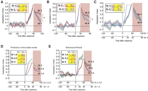
The history of prior experience affects the rate of decay of motor output. Yellow boxes in the force perturbation legends indicate the range of trials shown. A: adaptation indices in blocks 3 and 4 in groups 1 and 3. Prior experience with a rapidly changing environment increases decay rates as measured after an experience with a gradually changing environment. B: adaptation indices in blocks 3 and 4 in groups 2 and 4. Prior experience with a gradually changing environment slows decay rates as measured after an experience with a gradually changing environment. C: adaptation indices in blocks 3 and 4 in groups 1 and 4. Decays rates in these 2 groups are similar despite the fact that group 1 was just exposed to a gradually changing environment. D: predicted adaptation and retention of the sudden and maintained perturbation (group 5) in blocks 1 and 2 by the 2-state model and observed behavioral results as compared with a short, sudden perturbation (groups 1 and 4), and long gradual perturbation (groups 2 and 3). E: adaptation indices in blocks 1 and 2 in groups 1–5. Despite equal number of training trails, motor output decayed faster for group 5 than for groups 2 and 3.

We next tested whether a prior experience could similarly affect decay rates of memories that were acquired later in response to a sudden perturbation. One group initially experienced a gradually changing environment (group 2), and another group initially experienced a rapidly changing environment (group 4). After washout, they re-learned the same rapid perturbation. Performance during re-learning (Fig. 4B) was indistinguishable [F(1,17) = 0.517, P = 0.482]. Yet retention after re-learning was worse in the group that had previously observed a sudden perturbation [repeated-measure ANOVA, significant main group effect F(1,17) = 5.56, P < 0.05]. Indeed, the effect of the prior exposure to a sudden perturbation was remarkably strong: retention in group 1 after a gradual re-learning of perturbation was not significantly different from retention after a sudden perturbation in group 4 [Fig. 4C, F(1,17) = 0.08, P = 0.36].

In summary, despite a long period of washout between initial experience and re-learning, the initial experience had a strong influence on the decay rates of motor output following re-learning. If the initial experience was with a rapidly changing perturbation, it increased decay rates after re-learning. If the initial experience was with a gradually changing perturbation, it reduced decay rates after re-learning.

Control 1: number of trials

A great majority of adaptation experiments impose a sudden perturbation followed by a long period of trials that kept the perturbation constant. How is retention affected as compared with when a gradual perturbation is imposed over the same number of trials? That is, is the decay rate different when there are equal numbers of trials between the sudden and gradual protocols?

To answer this question, group 5 trained with a protocol that introduced the perturbation suddenly and maintained it for 50 trials. The main prediction from the two-state model is that in comparison to the gradual perturbation, the additional trials increase adaptation levels during training and result in superior performance during the following retention trials (Fig. 4D). As predicted, we observed that in group 5 the adaptation index during training (Fig. 4E) was significantly higher than in the gradual training groups [i.e., groups 2 and 3; F(1,22) = 52.184, P < 0.01]. However, contrary to predictions made by the two-state model, repeated-measure ANOVA showed a significant interaction effect between the protocols and movement bins [F(1,22) = 4.805, P = 0.039], suggesting that the motor output for group 5 decayed faster than for groups 2 and 3 (Fig. 4E).

We wondered whether the rapid perturbation in group 5 would bias the retention rates after re-learning. After the initial learning and washout, subjects in group 5 re-learned the field in a gradual protocol (Fig. 1B). The retention profile after re-learning (block 4) was not significantly different from the first retention profile within group 5 [block 2; F(1,14) = 0.527, P = 0.48], which is consistent with the results from other groups. We also compared the adaptation indices in the postrelearning retention trials with group 3 and found a trend toward a faster decay in group 5 though the differences were not significant [no significant group and movement bin interaction effect, F(5,70) = 1.078, P = 0.38, no main group effect, F(1,14) = 0.187, P = 0.672].

Control 2: the influence of the prior rate of change versus the direction of change

The data from groups 1–5 suggest that the exceedingly long washout block following initial learning did not really make the subjects naïve again: the prior experience affects the decay rates following re-learning. In other words, a group's retention behavior after relearning can be predicted by the retention behavior after initial learning. There are two competing scenarios that could explain this result. In the first scenario, despite the 120 washout trials, the slow state did not return to baseline. Rather in all groups that learned gradually in block 2, there was some residual slow state that lingered and aided re-learning and retention in block 4. This could explain the retention data in Figs. 3B and 4, A and B. However, this scenario could not explain the retention data in Figs. 3A and 4C. In a second scenario, the states return to zero but their decay rates maintain a memory of the rate of the change in the environment. The prior experience with the environment allows the learner to identify the environment as one with gradual changes. The learner reduces the decay rates, which encourages retention even if the environment now suddenly changes. That is, adaptation involves a system identification process that determines the structure, or pattern of the environment changes. In principle, this scenario can account for all the data in Figs. 3 and 4. Indeed, this scenario makes the rather unusual prediction that the factor that influences retention is the rate of change in the environment, not its specific contents. For example, it is irrelevant that in group 2, the initial learning was with a perturbation that was in the same clockwise direction as in re-learning (because the states washout completely in the subsequent washout phase). Rather, the crucial factor in the prior training of group 2 is the gradualness of change in perturbation during initial learning.

To directly test this idea, we recruited a new group of subjects (group 6) and in block 2 presented them with a gradual perturbation that was in the opposite (counter-clockwise) direction as all previous groups (Fig. 1B). Then to washout the learning, we followed this with 180 null trials. That is, the washout period was 3.6 times the learning period. Subsequently, the subjects were presented with a sudden perturbation opposite to the one that they had learned in block 2 (i.e., same perturbation in groups 1–5). The idea was that if the gradualness of the perturbation is the cause of better retention, then the subjects in group 6 should show better retention of the sudden field than block 2 of groups 1 and 4 or block 4 of group 4 despite the fact that their original learning was in the opposite field. Performance during the re-learning period of block 4 (Fig. 5A) was indistinguishable among groups 2, 4, and 6. However, retention was significantly better in group 6 than group 4 [Fig. 5A, main group effect, F(1,9) = 5.339, P = 0.032]. Indeed, retention of subjects in block 4 of group 6 was no different from block 4 of group 2 [no main group effect, F(1,16) = 0.222, P = 0.644], further demonstrating that the important common factor was the long prior exposure to a slowly changing environment. Retention in block 4 of group 6 was better than the naïve subjects in block 2 of group 1 [main group effect, F(1,16) = 6.101, P = 0.025] and group 4 [F(1,19) = 10.751, P = 0.004; Fig. 5B].

FIG. 5.

The history of prior experience affects the rate of decay of motor output. Yellow boxes in the force perturbation legends indicate the range of trials shown. A: adaptation indices in blocks 3 and 4 in groups 2, 4, and 6. Despite that group 6 initially adapted to an opposite force perturbation, the retention is significantly better for group 2 vs. 4 and for group 6 vs. 4 (repeated-measure ANOVA main effect, P < 0.05). B: adaptation indices in blocks 1 and 2 for groups 1 and 4, and blocks 3 and 4 for group 6. Retention is significantly better in group 6 vs. the 2 other groups.

Figure 6 summarizes the data with a bar plot that represents the average adaptation indices during the retention blocks. The decay rate of a recently acquired motor memory in a given environment was slowest if the prior experience in that environment did not include sudden changes.

FIG. 6.

Summary of the data in the retention phases of the experiment. Each bar is the across-subject average adaptation index during the error-clamp trials in the retention phase (yellow bar in the insets). The error bars are SE. The open bars are the indices during the 1st retention phase (block 2), and the gray bars are the indices in the 2nd retention phase (block 4). Note that group 5 is not plotted because their adaptation index immediately after learning was not the same as other groups and that group 6 had only 1 retention phase.

DISCUSSION

Our nervous system alters our motor output to maintain performance in a changing environment and with our changing body. Previous literature has suggested that we effectively learn by predicting the current state of the environment from our immediate past observations. Our results provide evidence that we also identify the statistics of change in environment from our past observations, and this in turn affects retention rates of the resulting memory.

Here we considered a task in which the state of the environment was a force that perturbed movements. The force sometimes stayed constant from trial to trial, sometimes changed suddenly, and sometimes changed gradually over many trials. To succeed, subjects needed to estimate this force and produce motor commands that countered it. We made three observations. 1) In naïve subjects in response to a sudden change in the force, the motor output changed rapidly but then also declined rapidly when performance errors were eliminated (i.e., error-clamp trials). In another group of naïve subjects, in response to a gradual change in the force, the motor output increased gradually but then also declined gradually. 2) After a long period of washout in which the force was returned to baseline, the prior training did not affect the rates of re-learning when the force once again changed. However, the prior training affected the decay rate after re-learning. Prior experience with a rapidly changing force encouraged faster forgetting even when re-learning involved a gradually changing force. Prior experience with a gradually changing force encouraged greater retention, even when re-learning included a rapidly changing force. 3) The critical factor in the prior experience was the rate of change in the environment not its direction of change. Therefore we found that we could readily alter the forgetting rate of an experience through manipulation of the prior experiences.

From a theoretical perspective, the new idea that emerges from our work is that learning is not merely a process of state estimation in which the brain uses a default generative model to optimally estimate the environment (Kording et al. 2007). Rather learning is a process of system identification in which we acquire a generative model that represents the environment, and we use that model to perform state estimation. What is surprising is that the process of system identification is evident even for short-term learning experiments that involve hundreds of trials, suggesting that it is highly flexible and responsive.

The results of our experiments demonstrate that time constants of the processes that support motor memory formation (i.e., matrix A in Eq. 7) cannot be constant but are themselves affected by the statistics of the learning experience. After experience with a slowly changing environment, the time constants shift toward slower time scales, whereas after experience with a rapidly changing environment, the time constants shift toward faster time scales. As a result, more of the prior experience is retained for slowly changing environments and more of it is forgotten for rapidly changing environments.

Our results shed some light on some puzzling observations in motor learning. One such observation has been that the adaptive response to a given error is consistently smaller in a randomly changing environment than in a nearly constant environment (Cheng and Sabes 2007; Donchin et al. 2003; Smeets et al. 2006; Smith 2004). One way to explain this is to posit that large errors carry less relevance than smaller errors, resulting in a smaller rate of learning (Wei and Kording 2009). However, our work suggests that a random environment encourages formation of a generative model that displays greater forgetting between trials, which would give the appearance of an adaptive system that learns less from errors.

In another example, it has been shown that the sensitivity to error is highest when the forces in the environment are highly correlated from trial to trial and lowest when the correlation is near zero (Smith and Shadmehr 2004). An environment with low trial-to-trial correlation is equivalent to one in which A in Eq. 6 is near zero, causing greater forgetting between trials, which would be equivalent to an adaptive system that appears to learn less from error.

A potential confound in our study was that to match performance levels at the end of learning period in groups 1 and 2, it was necessary to include more trials in the gradual protocol than the short and sudden protocol. That is, by the end of the initial learning period, the gradual protocol was longer in time than the sudden protocol. However, by the end of the re-learning phase, both groups 1 and 2 had been exposed to the same total exposure time and number of trials, yet they showed markedly different levels of motor ouputs. In group 5, the perturbation was introduced suddenly and maintained for 50 trials (equal number of trials as in the gradual group). However, we still observed a faster drop in motor output in group 5 than in groups that learned with the gradual protocol.

A second potential confound was that perhaps the extensive washout trials after the initial learning period were not long enough to return the slowest states to baseline (our washout trials were ∼3.6 times the length of the initial training). For example, this idea explains that in group 2, decay after re-learning was slow because the slow state did not washout. A strong test of this idea was in group 6 in which the initial training was in a gradually changing environment, but the direction of change during learning was opposite re-learning. We found that decay rates after re-learning were almost identical in groups 2 and 6 despite the fact that the initial learning was in opposite directions in the two groups. This result is consistent with the idea that the washout period returned the states to baseline, but altered the decay parameters of the adaptive process (i.e., a_f and a_s in Eq. 3].

A third potential confound was that the block of error-clamp trials itself introduced prediction errors in proprioception space (i.e., a spring force vs. a viscous force). These errors could in turn form the basis of learning contexts. For example, people could adapt differently to environments with different impedances (Burdet et al. 2001). In group 6, we removed the first block of error-clamp trials and still observed the same effects of gradual training observed in other groups. This indicates that a large contact force experienced in error-clamp trials did not significantly affect the rate of adaptation and de-adaptation in subsequent learning.

Our work here focused on decay properties of motor memories as a function of trial, rather than time. Our previous work demonstrated that these decay rates are distinct (Criscimagna-Hemminger and Shadmehr 2008) with passage of time having much smaller effects than trial. By focusing on the trial-dependent decay, we attempted to test the hypothesis that the decay rates of the putative fast and slow processes that appear to support motor learning were themselves plastic. Our results suggest that these decay rates are influenced by the second-order statistics of the learning experience.

In the current study, we have compared behavioral results against predictions of the two-state model. In another single-state model proposed by Emken et al., the forgetting factor is implemented to minimize effort (Emken et al. 2007). It is possible that a sudden change in the dynamics of the environment increases the instantaneous demand for effort with the consequence that trial-to-trial forgetting will be faster. Thus many sudden changes in the perturbation forces increase this demand further. Indeed Emken et al. show that the trial-to-trial forgetting is slower (0.76 ± 0.21) in an experiment with blocks of constant forces than in an experiment with blocks of different forces (0.64 ± 0.17). In this perspective, the Emken model, like the two-rate model, may functionally be sufficient to explain retention of a naïve learner after sudden or gradual training. However, the Emken model, like other one- or two-state models, assumes constant model parameters. Because of this property, it cannot account for the re-learning retention results in the current study. Taken together, we think the effect on the retention being reported in the current study speaks of a global phenomenon that can only be observed when one studies data beyond a single block of adaptation, much like with the savings studies.

It should be noted that in addition to the gradualness of perturbation exposure, the number of trials that have the same perturbation amount is likely to also have an influence in how learners construct the generative model of the environment. A sudden perturbation that lasts a few trials (e.g., group 4) may be different from a sudden perturbation that is followed by many “constant” trials (e.g., group 5) because trial-to-trial correlation of the perturbation state is much higher in the latter case. The fact that retention in group 3 (gradual learning and relearning) was only nonsignificantly higher than in group 5 in block 4 seems to suggest this. Nevertheless, the fact that retention was the same after learning and re-learning within any group we tested strongly supports the generative model hypothesis.

A main issue raised by recent models of motor learning is that when we observe a prediction error, we face a credit assignment problem (Kording et al. 2007; Smith et al. 2006). Is the change in the environment that caused this error likely to be sustained or is it transitory? Our results here suggest that the credit assignment policy may be based on a generative model that we acquire from the statistics of the performance errors. This generative model of the environment acts as a prior with which we estimate the state of the environment. In effect, forgetting rates are a reflection of our implicit estimate of the timescale of change in the environment.

GRANTS

The work was supported by National Institute of Neurological Disorders and Stroke Grants NS-037422 and NS-057814.

REFERENCES

- Baddeley et al. 2003.Baddeley RJ, Ingram HA, Miall RC. System identification applied to a visuomotor task: near-optimal human performance in a noisy changing task. J Neurosci 23: 3066–3075, 2003. [DOI] [PMC free article] [PubMed] [Google Scholar]
- Burdet et al. 2001.Burdet E, Osu R, Franklin DW, Milner TE, Kawato M. The central nervous system stabilizes unstable dynamics by learning optimal impedance. Nature 414: 446–449, 2001. [DOI] [PubMed] [Google Scholar]
- Burge et al. 2008.Burge J, Ernst MO, Banks MS. The statistical determinants of adaptation rate in human reaching. J Vis 8: 20 21–19, 2008. [DOI] [PMC free article] [PubMed] [Google Scholar]
- Cheng and Sabes 2007.Cheng S, Sabes PN. Calibration of visually guided reaching is driven by error-corrective learning and internal dynamics. J Neurophysiol 97: 3057–3069, 2007. [DOI] [PMC free article] [PubMed] [Google Scholar]
- Criscimagna-Hemminger and Shadmehr 2008.Criscimagna-Hemminger SE, Shadmehr R. Consoidation patterns of human motor memory. J Neurosci 28: 9610–9618, 2008. [DOI] [PMC free article] [PubMed] [Google Scholar]
- Donchin et al. 2003.Donchin O, Francis JT, Shadmehr R. Quantifying generalization from trial-by-trial behavior of adaptive systems that learn with basis functions: theory and experiments in human motor control. J Neurosci 23: 9032–9045, 2003. [DOI] [PMC free article] [PubMed] [Google Scholar]
- Emken et al. 2007.Emken JL, Benitez R, Sideris A, Bobrow JE, Reinkensmeyer DJ. Motor adaptation as a greedy optimization of error and effort. J Neurophysiol 97: 3997–4006, 2007. [DOI] [PubMed] [Google Scholar]
- Ethier et al. 2008.Ethier V, Zee DS, Shadmehr R. Spontaneous recovery of motor memory during saccade adaptation. J Neurophysiol 99: 2577–2583, 2008. [DOI] [PMC free article] [PubMed] [Google Scholar]
- Hatada et al. 2006.Hatada Y, Miall RC, Rossetti Y. Two waves of a long-lasting aftereffect of prism adaptation measured over 7 days. Exp Brain Res 169: 417–426, 2006. [DOI] [PubMed] [Google Scholar]
- Huang and Shadmehr 2007.Huang VS, Shadmehr R. Evolution of motor memory during the seconds after observation of motor error. J Neurophysiol 97: 3976–3985, 2007. [DOI] [PubMed] [Google Scholar]
- Huang et al. 2008.Huang VS, Shadmehr R, Diedrichsen J. Active learning: learning a motor skill without a coach. J Neurophysiol 100: 879–887, 2008. [DOI] [PMC free article] [PubMed] [Google Scholar]
- Hwang et al. 2006.Hwang EJ, Smith MA, Shadmehr R. Adaptation and generalization in acceleration-dependent force fields. Exp Brain Res 169: 496–506, 2006. [DOI] [PMC free article] [PubMed] [Google Scholar]
- Joiner and Smith 2008.Joiner WM, Smith MA. Long-term retention explained by a model of short-term learning in the adaptive control of reaching. J Neurophysiol 100: 2948–2955, 2008. [DOI] [PMC free article] [PubMed] [Google Scholar]
- Kagerer et al. 1997.Kagerer FA, Contreras-Vidal JL, Stelmach GE. Adaptation to gradual as compared with sudden visuo-motor distortions. Exp Brain Res 115: 557–561, 1997. [DOI] [PubMed] [Google Scholar]
- Klassen et al. 2005.Klassen J, Tong C, Flanagan JR. Learning and recall of incremental kinematic and dynamic sensorimotor transformations. Exp Brain Res 164: 250–259, 2005. [DOI] [PubMed] [Google Scholar]
- Kluzik et al. 2008.Kluzik J, Diedrichsen J, Shadmehr R, Bastian AJ. Reach adaptation: what determines whether we learn an internal model of the tool or adapt the model of our arm? J Neurophysiol 100: 1455–1464, 2008. [DOI] [PMC free article] [PubMed] [Google Scholar]
- Kording et al. 2007.Kording KP, Tenenbaum JB, Shadmehr R. The dynamics of memory as a consequence of optimal adaptation to a changing body. Nat Neurosci 10: 779–786, 2007. [DOI] [PMC free article] [PubMed] [Google Scholar]
- Michel et al. 2007.Michel C, Pisella L, Prablanc C, Rode G, Rossetti Y. Enhancing visuomotor adaptation by reducing error signals: single-step (aware) versus multiple-step (unaware) exposure to wedge prisms. J Cogn Neurosci 19: 341–350, 2007. [DOI] [PubMed] [Google Scholar]
- Reisman et al. 2007.Reisman DS, Wityk R, Silver K, Bastian AJ. Locomotor adaptation on a split-belt treadmill can improve walking symmetry post-stroke. Brain 130: 1861–1872, 2007. [DOI] [PMC free article] [PubMed] [Google Scholar]
- Scheidt et al. 2000.Scheidt RA, Reinkensmeyer DJ, Conditt MA, Rymer WZ, Mussa-Ivaldi FA. Persistence of motor adaptation during constrained, multi-joint, arm movements. J Neurophysiol 84: 853–862, 2000. [DOI] [PubMed] [Google Scholar]
- Shadmehr and Mussa-Ivaldi 1994.Shadmehr R, Mussa-Ivaldi FA. Adaptive representation of dynamics during learning of a motor task. J Neurosci 14: 3208–3224, 1994. [DOI] [PMC free article] [PubMed] [Google Scholar]
- Smeets et al. 2006.Smeets JB, van den Dobbelsteen JJ, de Grave DD, van Beers RJ, Brenner E. Sensory integration does not lead to sensory calibration. Proc Natl Acad Sci USA 103: 18781–18786, 2006. [DOI] [PMC free article] [PubMed] [Google Scholar]
- Smith et al. 2006.Smith MA, Ghazizadeh A, Shadmehr R. Interacting adaptive processes with different time scales underlie short-term motor learning. PLoS Biol 4: e179, 2006. [DOI] [PMC free article] [PubMed] [Google Scholar]
- Smith and Shadmehr 2004.Smith MA, Shadmehr R. Modulation of the rate of error-dependent learning by the statistical properties of the task. Adv Comput Mot Control vol. 3, San Diego, 2004.
- Wei and Kording 2009.Wei K, Kording K. Relevance of error: what drives motor adaptation? J Neurophysiol 101: 655–664, 2009. [DOI] [PMC free article] [PubMed] [Google Scholar]