Abstract
Mathematical Principles of Reinforcement (MPR) is a theory of reinforcement schedules. This paper reviews the origin of the principles constituting MPR: arousal, association and constraint. Incentives invigorate responses, in particular those preceding and predicting the incentive. The process that generates an associative bond between stimuli, responses and incentives is called coupling. The combination of arousal and coupling constitutes reinforcement. Models of coupling play a central role in the evolution of the theory. The time required to respond constrains the maximum response rates, and generates a hyperbolic relation between rate of responding and rate of reinforcement. Models of control by ratio schedules are developed to illustrate the interaction of the principles. Correlations among parameters are incorporated into the structure of the models, and assumptions that were made in the original theory are refined in light of current data.
Keywords: Reinforcement, Arousal, Constraint, Association, Coupling, Ratio schedules
1. Introduction
Principles are the skeleton of a theory; models provide the muscle. Principles guide the growth of models; models put the principles into contact with data. Principles are stated in general terms; models engage the particulars. Parameters of the models describe the state of the organism by further restricting the degrees of freedom of the theory. As an example, the equation of motion for a point particle may be based on Newton’s principles; the relevant model may be the mathematical machinery that describes the motion of the particle toward and through a hollow sphere; the parameters may involve the gravitational constant, characteristics of the sphere and particle, and the initial conditions of distance and motion.
If a skeleton is ill suited for a task, the muscles can compensate up to a point. But too heavy a load will eventually break one or the other. Correctly aligned skeletons permit simpler and more efficient musculature. This paper dissects a theory of behavior called Mathematical Principles of Reinforcement (MPR; Killeen, 1994). It articulates the three main principles that constitute its skeleton: motivation, association and constraint. It overlays the principles with models that provide the detail necessary to describe data. Finally, it realigns the way in which the models instantiate the principles, to more accurately reflect patterns in the data, and to render the parameters more descriptive of the principles they represent.
2. The principles
Reinforcement empowers and directs behavior. It empowers it by generating a heightened state of arousal, one that can become conditioned to the context in which reinforcement occurs. It directs behavior by selecting from among the responses it instigates those that immediately precede and predict it. That arousal and direction acts under the constraint of finite time and energy available to execute a response.
2.1. Motivation/activation/arousal
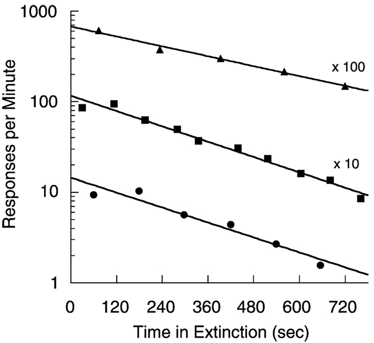
Killeen, Hansen and Osborne (1978) placed pigeons in an enclosure with floor panels that measured their activity, fed them once, and returned them to their home cages after half an hour. Fig. 1 shows that the pigeons became active upon the delivery of food, and settled down slowly thereafter. The straight lines in these semi-log coordinates indicate that the settling proceeds according to an exponential decay function: b(t) = b1e−t/α. The average parameters from these conditions are the intercept b1 = 9.7 responses/min, and the time constant α = 6 min. The total number of responses after such incitement is the integral of the exponential function, αb1.
Fig. 1.
The average rate of activation of floor panels in three experiments in which hungry pigeons were given one feeding per day, shown as a function of time since that feeding. The top two curves are offset by the factors noted. Straight lines in these semi-logarithmic coordinates evidence exponential decay of activity. From Killeen et al. (1978).
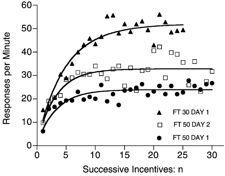
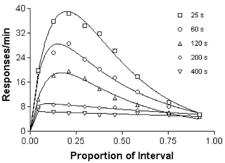
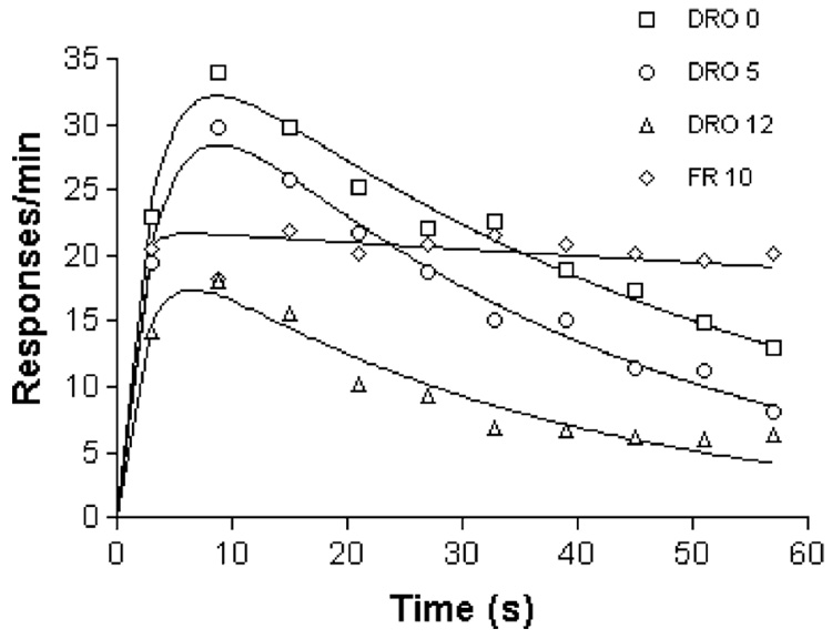
In the next experiment, the frequency of feeding was increased from daily to every FT seconds. Fig. 2 shows that activity increased to well above the levels manifest in the one-trial per day conditions. Was the elevation of the asymptotes due to the operant reinforcement of general activity? If so, a contingency making reinforcement unavailable within 5 s of a report from the activity sensors (a DRO 5 s) should eliminate superstitious activity. Fig. 3 shows the limited effectiveness of the DRO: activity decreased before reinforcement; but it remained at high levels in the earlier part of the inter-reinforcement interval. Were the DRO contingency ineffective we would not see the decrease; were the activity maintained solely by adventitious pairing with food, we would not see the increase before the decrease.
Fig. 2.
When shifted to periodic feedings, pigeons’ response rates increase toward their asymptote with each feeding. From Killeen et al. (1978).
Fig. 3.
The average rate of activation of floor panels in an experiment in which hungry pigeons were fed every t seconds, with t = 25, 60, 120, and 200 and 400 s, displayed over a normalized x-axis. Food was withheld until 5 s had elapsed without measured activity. The curves through the data are generalized Erlang distributions. From Killeen (1975).
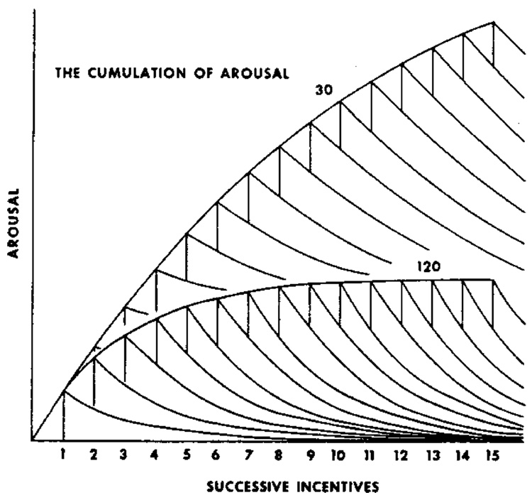
The asymptotic level of activity in these figures appears related to the rate of feeding. It is as though the activity curves in Fig. 2 were stacked atop one another, as shown in Fig. 4. Periodic feeding makes the animal increasingly excited, as though the excitement itself cumulates, and does so increasingly with increasing frequency of reinforcement. Needing a name for this state of excitement, we call it arousal.
Fig. 4.
Driving the system with periodic reinforcement may cause arousal to cumulate. From Killeen et al. (1978).
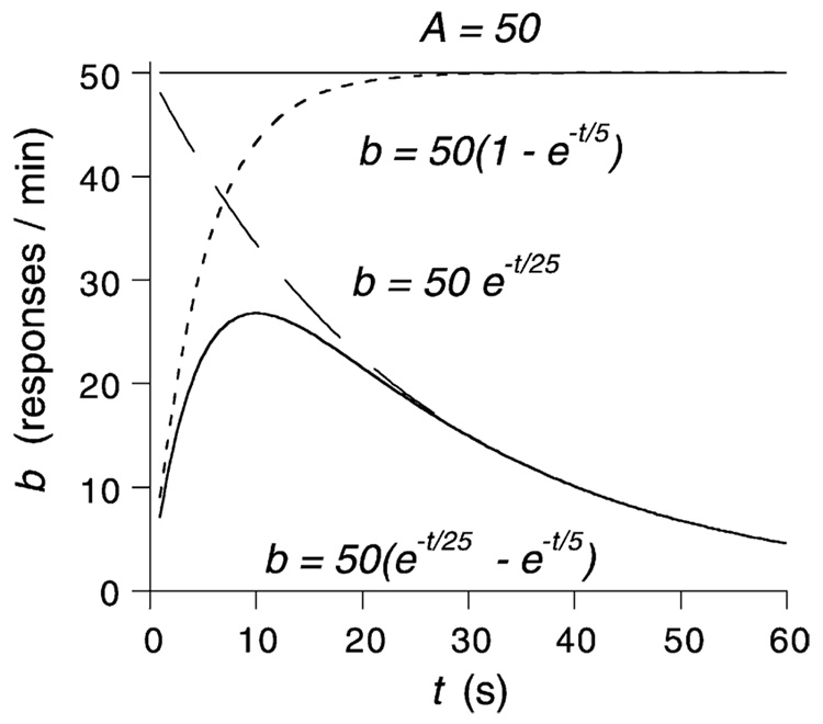
Average response rates increase with the rate of reinforcement, but they also change as a function of other variables—DRO contingencies, hopper approach, and other factors. This is shown in Fig. 5, where responding on a schedule of periodic food presentation was suppressed with increasingly severe DRO contingencies, or encouraged with contingent reinforcement (every 10th response after the time elapsed was followed with reinforcement: an FR 10 schedule). To generate a cleaner measure of asymptotic arousal, the temporal trends in data such as those shown in Fig. 3 and Fig. 5 were removed by fitting a theoretical model, the generalized Erlang distribution, to them. This distribution has been used to characterize timing processes (McGill and Gibbon, 1965), and here captures the idea that animals engage in focal search around the hopper after a feeding (Timberlake and Lucas, 1990), remaining relatively stationary for a period of time that is exponentially distributed with mean 1/β. Thereafter, a period of more-or-less vigorous general search lasts for an exponentially distributed random time with mean 1/γ, followed by another epoch of focal search (“goal tracking”). When measured by proximity switches, the epochs of focal search reveal responding whose temporal pattern is complementary to general activity (Killeen, 1979, Fig. 2.11). If we look into the box at time t, we shall find the animals engaged in general search with a probability proportional to e−βt – e−γt, shown in Fig. 6. This is the function drawn through the data in Fig. 3 and Fig. 5. It accurately describes the time course of general activity and other adjunctive activities of pigeons, rats and chickens (Killeen, 1975).
Fig. 5.
Imposition of contingencies to discourage responding (DRO) does not eliminate activity. From Killeen (1975).
Fig. 6.
The logic of the model of temporal control. A very slowly decaying level of arousal (A) is approximated by the straight line at 50. General activity is inhibited immediately after reinforcement, probably due to hopper-related activity. The inhibition dissipates exponentially, releasing the animal to move about as shown by the dotted curve. Subsequently, attention to the front panel and the hopper grows exponentially with time, depressing general activity as shown by the dashed curve. Squeezed between these forces, general activity follows the bitonic time course shown here and in Fig. 3.
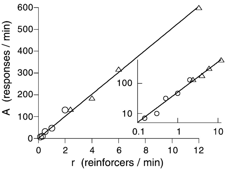
The exponential processes account for the patterning in the data, leaving the scale factor A freedom to reflect the asymptotic level of activity that would occur in absence of the competition from goal tracking and other forces that draw the animals into responses that do not register on the monitors. It is not that animals are less aroused toward the end of interfood intervals; rather, our monitors are differentially sensitive to certain response topographies. We take the vigor of the activity we measure as an index of arousal. The asymptote of the activity curves shown in Fig. 6, A, increases as a linear function of the rate of feeding, as shown in Fig. 7. An increase is consistent with the model of the cumulation of arousal shown in Fig. 4. The function entailed by that graphical model requires the average level of arousal to increase as An = A1αr(1 − e−n/αr). A1 is the jolt of arousal engendered by a reinforcer, which is proportional to the intercept of the curves shown in Fig. 2, α the time constant of those curves, r the rate of reinforcement, and n the number of reinforcers. As n increases, the asymptotic arousal approaches A∞ = A1αr. This may be written as A = ar, with the parameter a standing for A1α. The asymptote A is the same for both fixed and variable interincentive intervals (Killeen and coworkers, 1978).
Fig. 7.
Asymptotic response rates inferred from the model shown in Fig. 4 when applied to the data from Fig. 3 (open circles) and from another study reported in (Killeen, 1975). The inset shows the same data in logarithmic coordinates. The linear increase is predicted by the model shown in Fig. 4 and Fig. 6 (see Killeen et al., 1978, for details).
In MPR a is called specific activation. Both arousal level (A = ar) and specific activation (a) are hypothetical constructs referring to motivational states (A) and to the power of a single reinforcer, of a particular type, applied to a particular organism, at some level of deprivation (a), to induce responding. As hypothetical constructs, they cannot generally be measured directly. The simplest way to connect them to behavior is to assume that response rate is proportional to arousal level, with a constant of proportionality k responses per second. Because k is not measurable, it is simply absorbed into a, changing the dimensions of that parameter from seconds per reinforcer to responses per reinforcer. Then a becomes the integral of the exponential decay curves in Fig. 2. That area under the curves is the total activity elicited by a single reinforcer, measured by a transducer with a sensitivity characterized by k. This construction ties a to the particular response under consideration, as different responses are often differentially sensitive to reinforcement (Killeen, 1979, Fig. 2.13), and differentially affect a particular transducer. The data from Fig. 1–Fig. 4 were collected with the same floor panels with the same sensitivity k, and thus permitted the prediction of the data shown in Fig. 7. In Nevin’s (1992, 2002) theory a construct similar to A is called momentum (Nevin, 1994, 2003; Killeen, 2000). In Skinner’s (1938) theory a was called the reflex reserve (Killeen, 1988). These issues are treated in more detail in Killeen (1979, 1998), and below.
The above considerations are epitomized in The first principle of reinforcement: arousal (A) is proportional to the rate of reinforcement: A = ar. The constant of proportionality, a, is called specific activation.
Response rates may vary considerably even while the motivational state (A) remains unchanged. In the experiments whose results appear in Fig. 5, for instance, neither deprivation level nor quality of reinforcer varied across conditions, so that specific activation, a, was constant, and rate of reinforcement was relatively constant. Yet response rates fell well below their theoretical asymptote A, and varied substantially due to the contingencies that reinforced or punished the target response. Two additional factors must be considered in translating arousal level into measured rates of target responding. The first is competition from other responses, both from the same operant class and from competing classes (such as focal search). The other factor is the contingency that selects which operant class, target or some other, is strengthened by reinforcement and details the topography of that class. Fig. 6 showed one way of parsing competing classes of responses. The following section deals with competition from responses of the same class. The issue of contingencies, and how they focus arousal on the target response, or on a mixture of responses, constitutes the matter of the third principle, and is discussed below.
2.2. Constraint
The first principle related rate of reinforcement to arousal level on one hand and to response rate on the other. The simplest relation between responding and arousal—proportionality—was assumed, with the constant k a feature of the measuring apparatus and absorbed into a. This works at low response rates, such as those shown in Fig. 1. But Fig. 3 and Fig. 6 show that competition from other responses may cause response rate to fall short of its theoretical asymptote A. Another reason it may fall short is because it takes time to make a response, and therefore, responses cannot be emitted as fast as they are elicited. The average response rates in the experiments that provided the data in Fig. 7 did not differ very much at the highest rates of reinforcement; there is a maximum rate at which animals can move about the chamber, and as they approached this rate, increasing reinforcement frequency was of decreasing efficacy in increasing response rates.
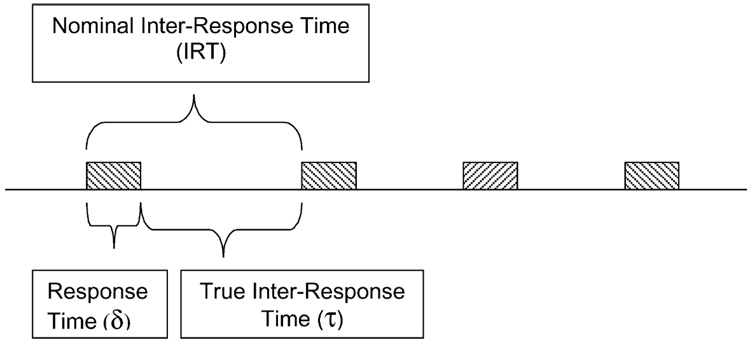
Response rate is a classic, robust, and valid dependent variable (Killeen and Hall, 2001). It is measured by counting the number of target responses within an epoch and dividing that number by the duration of the epoch. This gives rate of responding, b, the reciprocal of the average time from the start of one response to the start of the next. This is traditionally called the interresponse time (IRT). But measured this way it is not what its name suggests—the time between responses—but rather the cycle time, the time from the start of one response to the start of the next. The IRT comprises two subintervals, the time required to emit the response, δ (delta) plus the time between responses, τ (tau, the literal inter-response time; see Fig. 8, and Table 1 for a list of symbols). There is an obvious ceiling on rates measured as responses divided by observation interval: if the observation interval is 1 s, the time available for the first response is 1 s; the time available for a second response is τ = 1−δ s. For an animal responding at the rate of b responses per second, the average time available for an additional response is τ = 1 − bδ. As b approaches 1/δ, the observation epoch becomes filled with responses, and it is difficult or impossible for the animal to squeeze in additional responses. The maximum response rate is thus bmax = 1/δ.
Fig. 8.
The decomposition of an IRT into its components: delta, the time required to complete a response, and tau, the time between responses.
Table 1.
Mathematical symbols and their explanations
| Symbol | Name | Meaning | Constituent |
|---|---|---|---|
| a | Specific activation | The number of responses of duration δ that will be supported by a particular incentive under a particular level of deprivation | a = kνm where k is a scale factor, ν measures the value of an incentive, and m measures motivation of the organism Killeen (1995) |
| A | Arousal level | Governs asymptotic responses rate, when characteristics of the sensor, duration of a response, and competition from other responses are taken into account | A = ar where a is specific activation, and r is rate of reinforcement Killeen (1994, 1998) |
| δ | Delta; response duration | The minimum time required for a single response cycle | b = 1/(τ + δ) where b is response rate and τ is time between responses (Fig. 8) |
| c. | Coupling coefficient | The degree of association between responses of the same operant class and reinforcement. Its expected value depends on the schedule of reinforcement and rate of responding; it was symbolized ζ in Killeen (1994) | where b(t) = 1 while a target response is in progress and 0 otherwise |
| β | Beta | The proportion of the maximum association conferred on the response that immediately precedes reinforcement | β = 1 − e−λδ |
| λ | Lambda | The rate of decay of response traces |
It follows that there are two ways to measure response rate: traditionally, as the number of responses divided by the observation interval: b = 1/(δ + τ), where δ is the average response duration and τ is the average time between responses; or as the number of responses divided by the time available for responding: 1/τ; this is sometimes called the instantaneous rate. At low rates of responding where τ ≫ δ the two measures are essentially equal. At high rates of responding b must bend under its ceiling, never to exceed 1/δ. Response rate measured as b is thus an inverse function of δ; 1/τ is not so constrained. In the parlance of cognitive psychology, b is a confound of both motor (δ) and decision (1/τ) processes. Because the nature of the operandum is arbitrary, and may change by accident or design within the course of an experiment, the instantaneous rate 1/τ may be the best way to measure response rate.
Killeen et al. (2002) developed a map between response rate and probability. They showed that if the probability p of observing a response in a small interval of time is proportional to arousal level, then the instantaneous response rate 1/τ will also be proportional to A. By definition A = ar, so 1/τ = ar; and inversely τ = 1/ar. This proportionality between the expected time between responses, τ, and the expected time between reinforcers, 1/r, is a premise of linear systems theory (McDowell et al., 1993). It has the advantage of being one of the simplest possible relations between input and output of any system.
Remember that the conventional measure of rate of responding, b, equals 1/(δ + τ). If, as suggested above, τ = 1/ar, then b = 1/(δ + 1/ar). Rearranging:
| (1) |
Eq. (1) forms the basis of the final equations of prediction of MPR. It formalizes the idea that while responses may be elicited at a rate proportional to A = ar, they can only be emitted at a rate of b due to the time it takes to make them. As δ → 0, b → ar. The addends in the denominator have the dimension of number of reinforcers per response, and the numerator the dimension of number of reinforcers per second. This is slightly different than the form given in Killeen (1994), as explained in Section 3.3.
Notice what happens to Eq. (1) if we call 1/δ “k”, and 1/δa “r0”:
| (2) |
Eq. (2) shows that this treatment of temporal constraint yields Herrnstein’s hyperbola (Herrnstein, 1970, 1979), as also shown by Staddon (1977).
2.2.1. Relation to other models
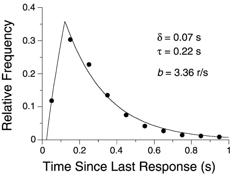
Eq. (1) is the same as the correction applied to data from counters in which each recorded response blocks the machine’s ability to register additional responses for δ s (Bharucha-Reid, 1960). If responses are elicited with constant probability within the epoch, then the IRT distribution consists of quiescence for δ s after a response followed by an exponential waiting time to the emission of the next response. This model provides a good account of the lever-press responses of rats, as seen in Fig. 9. In that figure, the relative frequency of a rat’s IRTs in 0.10 s bins are plotted against the IRT. If the bins were of size δ s, the relative frequency of responses in the first bin would be 0.0, and thereafter decay exponentially. In Fig. 9, the first bin comprises 0.07 s of refractory period plus 0.03 s of the shortest (high frequency) IRTs, yielding the observed intermediate frequency. The survivor function of this distribution (Shull, 1991) is a straight line in semi-logarithmic coordinates, with an x-axis offset of δ s. The key-pecking of pigeons follows a roughly similar course, but close analysis often shows periodic ripples in the function (Killeen et al., 2002; Palya, 1992). The inability of organisms to emit measurable responses of zero duration causes the offset of the exponential decay from the origin by δ s, and requires Eq. (1) as a corrective. This analysis thus ties Herrnstein’s hyperbola to the microstructure of responding. Eq. (1) plays the same role in the analysis of behavior as the Lorentz transformation does in mechanics: both are corrections for ceilings on the rate of motion—ceilings of 1/δ for the speed of an animal’s response, and c for the speed of a body’s movement.
Fig. 9.
The frequency with which different IRTs were emitted by a rat reinforced for every 80th response. The descending curve is an exponential decay function, consistent with a constant-probability emitter with a dead time of δ s. The rising curve plots the expected frequency of observation of IRTs in the interval Δ, as Δ increases from 0 to 0.1 s, plotted over abscissae of x = Δ/2. This figure shows the empirical relation between b = 1/IRT, δ, and τ, the rate of decay of the exponential. From Killeen et al. (2002).
This section has given us The second principle of reinforcement: response rate (b) is constrained by the time required to emit a response (δ). Eq. (1) corrects for the difference between the rate at which responses are elicited by reinforcement and the rate at which they can be emitted by the organism.
2.3. Coupling
How does the delivery of an incentive change the velocity of behavior? Velocity is a vector whose length measures speed and whose orientation indicates direction. Both are affected by how the incentive is scheduled with respect to the target responses, a relationship Skinner called the contingency of reinforcement. Galbicka and Platt (1986) showed that contingencies exercised substantial control over response rates independently of reinforcement rate effects. This section develops those insights into models.
2.3.1. Direction
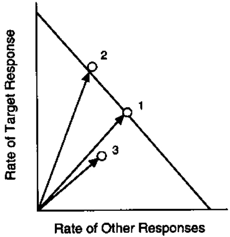
Consider the behavior-systems theory of Timberlake (e.g. Timberlake and Lucas, 1990), which enlists ethograms of organisms’ actions. Select one action as a target response—that is, a response to be measured and reinforced—and plot its rate on the vertical axis of a graph. Plot the rate of other responses on the horizontal axis (see Fig. 10). The maximum response rates for a given level of arousal will fall along a diagonal iso-arousal line, which has intercepts of 1/δy and 1/δx. Changes in A will change the distance of the diagonal from the origin, as shown by Vectors 1 and 3. The y-intercept is given by Eq. (1). The x-intercept is given by Eq. (1) written for responses measured and reinforced independently of the target response.
Fig. 10.
Target (reinforced) response rates are plotted against rates of other responses in this state space. The diagonal is an iso-arousal contour, which shows the possible allocation of responses for a given level of arousal. Increases in arousal level move the diagonal out from the origin, up to the limiting constraint line when all available time is filled with responding (e.g. from 3 to 1). Contingencies of reinforcement move the operating point toward or away from the vertical (e.g. from 1 to 2).
Reinforcement that is tightly associated with the target response will drive behavior primarily up the vertical axis. In such cases, coupling to, or correlation with, the target response, c, may approach +1.0. Vector 2 shows the effect of an increase in coupling to the target response compared to Vector 1. Reinforcement that is independent of the target response (c = 0) will drive behavior primarily along the horizontal axis. Reinforcement of behavior that is incompatible with the target response (c < 0, as the case for the DRO contingencies shown in Fig. 5), drives behavior down the vertical axis.
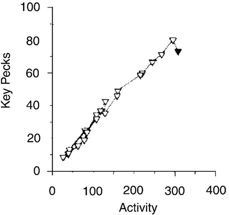
Changes in drive level affect specific activation a (Killeen, 1995), but may leave coupling invariant. The satiation of pigeons working on a schedule in which key-pecks were followed with 10-s access to food every 90 s generated the trajectory shown in Fig. 11. The x-axis shows general activity as measured with a standard stabilimeter. The direct descent of the trajectory to the origin shows that coupling was not affected by drive level. Decreasing rate of reinforcement, however, may generate a curvilinear descent to the origin (e.g. Killeen and Bizo, 1998, Fig. 12), indicating a change in coupling along with the decrease in arousal level.
Fig. 11.
Average satiation trajectory from six pigeons pecking a key for large amounts of food (Killeen and Bizo, 1998). Data from the first 10-min of the session are indicated by the filled triangle, and each 10 min thereafter by the open triangles. The linear descent to the origin indicates a decrease in arousal with little change in coupling.
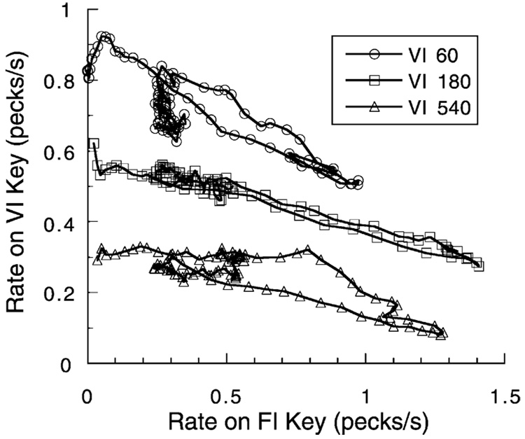
Changes in the coupling between the target response and reinforcer will move behavior along the iso-arousal diagonal. This is shown in Fig. 12, where pigeons could respond on one key for food every 30 s (an FI 30-s schedule) or on another key to receive food randomly every 6 s. Trials lasted for 100 s, with food scheduled for one or the other key probabilistically on each trial. The trajectories start at the left axis and follow a diagonal down to the lower right, returning after 30–45 s to an intermediate position. As the trial continues and it becomes obvious that the periodic food will not be obtained, the probability of reinforcement decreases; the reduced arousal level returns behavior over a lower trajectory which may, in the end, dwindle toward the origin, as seen in the top trajectory.
Fig. 12.
Rates of pecking at a key providing food randomly every VIs on the average are plotted as a function of rate of pecking a second key providing food periodically every 30 s. The data are averages over one session for three pigeons, collected in trials lasting 100 s. Most movement is along iso-arousal contours, but deviation from diagonals indicates decreases in arousal during the last half of the trials. From Killeen (1992).
2.3.2. Calculation
Coupling, as displayed in these figures, involves the association of a class of responses with a reinforcer. It may be measured post hoc as the cosine of the angle a response vector makes with the y-axis. Or, it may be predicted from knowledge of the contingencies of reinforcement.
Sometimes the reinforcer is not controlled by the experimenter: rats spend a substantial portion of the first 10 min of a session exploring the chamber, so when the x-axis is a measure of general activity, their behavioral trajectories always start with a lead from the right (Killeen and Bizo, 1998). Sometimes coupling varies over time, as displayed in Fig. 12. But to a large extent coupling is under the control of the experimenter. Schedules of reinforcement specify the requirements for the delivery of a reinforcer; it is possible to calculate the degree to which they will be effective in coupling the target response to the reinforcer. To do this requires an assumption about the nature of the association, introduced in Fig. 13. The essence of the assumption is captured by the Third Principle: the coupling between a response and reinforcer decreases with the distance between them. This distance may be measured in space, in time, or in number of intervening events; the decrease in coupling (the “response trace” or “delay of reinforcement gradient”) may be of any concave shape; here it is assumed to be exponential. Coupling is assumed to function by increasing the probability of whatever responses are present in memory at the time of reinforcement (Killeen, 2001; cf. Lattal and Abreu-Rodrigues, 1994).
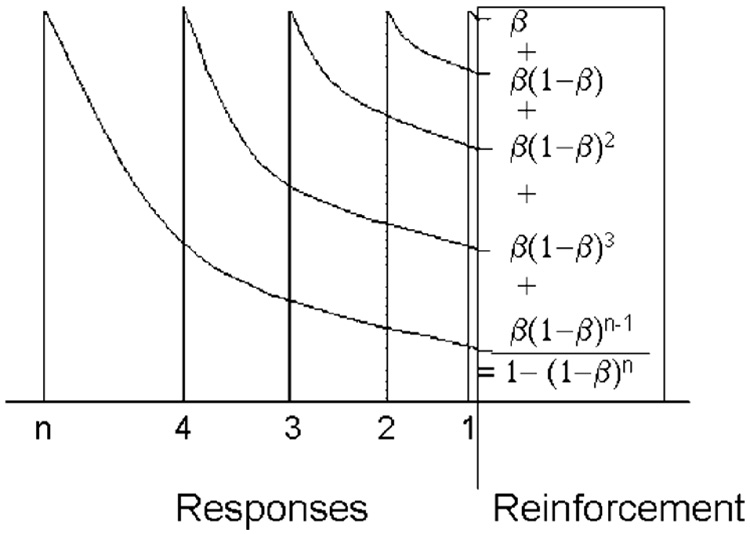
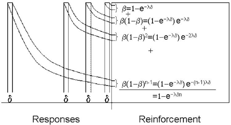
Fig. 13.
Reinforcement strengthens not only the last response but also prior ones, to a decreasing extent as they are remote from the reinforcer, illustrating the third principle of reinforcement. The equations within the reinforcement epoch represent the calculation of the coupling coefficient as the summation of the traces of the target responses.
What does reinforcement strengthen? All reinforceable (Shettleworth, 1975) responses that precede it. These include consummatory, post-consummatory, adjunctive and instrumental target responses (Lucas et al., 1990). Reinforcement may even strengthen responses that preceded the prior reinforcer, if those are recent enough relative to the delay gradient. Consummatory and post-reinforcement responses are not measured as target responses, yet they displace the memory for earlier target responses. Killeen and Smith (1984) called such displacement “erasure”; they showed that the delivery of reinforcement decreased pigeons’ ability to subsequently discriminate whether their target responses caused the delivery of the reinforcer. This overshadowing increased with the duration of the reinforcer up to durations of 4 s, where discrimination approached chance. Consider the implication for the simplest of reinforcement schedules, the fixed ratio (FR) schedule, which follows every nth response with reinforcement. In Fig. 13, one such reinforcer is shown intercepting the traces of five responses: the rightmost which triggered reinforcement, and four prior responses. Each response receives the proportion b of the available associative strength. The last response receives the proportion β of the maximum (1.0), leaving 1 − β for the remaining responses. The penultimate response receives β(1 − β); the third back receives β(1 − β)2. The nth back receives β(1 − β)n−1. If these responses are all from the same class, that of the target response, that class will be strengthened by the sum of this series, which is 1 − (1 − β)n. This is the discrete coupling coefficient for FR schedules, cFR. (Killeen (1994) used the symbol ζ for the coupling coefficient; that is changed here for mnemonic and orthographic convenience.) As the number of prior target responses n gets very large, coupling to the target response approaches 1.0. For an FR 5 schedule and β = 0.25, this is 1–0.755 = 0.76. It is not 1.0 because the five recorded target responses are preceded by consummatory and postprandial responses. The subsequent reinforcer strengthens the memory of these goal-oriented responses, with the potential impact on still earlier target responses muted by the intervening reinforcement. If this sidetracking of memory from target response to consummatory response is complete, coupling is truncated at the ratio value.
How does coupling enter the equations of motion? It tells us how arousal is associated with the target response. But reinforcement can only act on behavior that is manifest, and so it must modulate response rates, not arousal level. The simplest implementation is to multiply Eq. (1) by the coupling coefficient:
| (3) |
Eq. (3) is the fundamental model of MPR. It predicts measured target response rates will equal the product of the coupling coefficient (c.) with the response rate that is supported by that rate of reinforcement (from Eq. (1)). The dot in the symbol for coupling coefficient is a place holder for the designation of the particular contingencies under study.
On FR schedules it is trivial to predict response rates (b) from reinforcement rates (r), because, by definition of the schedule, r is proportional to b: r = b/n, where n is the ratio requirement. This relation is called the schedule feedback function (Baum, 1992). For a true prediction, substitute this schedule feedback function into Eq. (3) in place of r, and solve for b. The result is the equation of motion under ratio schedules:
| (4) |
where c. is the coupling coefficient for the ratio schedule in force. For FR schedules, we saw that:
| (5) |
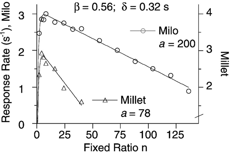
This model provides an accurate account of the response rates of pigeons under FR schedules (see, e.g. Bizo and Killeen, 1997; cf. Baum, 1993). The virtual y-intercept (extrapolated to 1/δ when n = 0) changes with changes in the nature of the response, and the slope (−1/δa) changes with changes in specific activation, and is also affected by response duration. The x-intercepts are found by setting b = 0 and solving for n. The first intercept occurs when n (and therefore cFR0) = 0. The other intercept, Skinner’s extinction ratio, occurs when n = cFRna. On large ratio schedules cFRn approaches 1, so rates go to 0 as n approaches a. This is consistent with the original definition of a as the average number of target responses that a reinforcer can maintain. These parameters can be seen at work in Fig. 14, which shows the response rates of four pigeons on FR schedules with 5 s of access to different grains as reinforcers. The rate of trace decay, β, and minimum response time δ are the same for both conditions. The value of a is significantly greater for milo than millet. Milo is known to be a preferred grain (Killeen et al., 1993).
Fig. 14.
Pigeons’ response rates on FR schedules of reinforcement with milo (left axis) or millet (right axis; notice the axis break). Data from Bizo and Killeen (1997). Projection of the linear portion gives y-axis intercepts of 1/δ = 3.1 responses/s, and x-axis intercepts of a = 78 for millet and 200 for the larger milo grain.
On random ratio schedules in which each response has a probability of 1/VR of being reinforced, the coupling coefficient is the average of the coefficients of FRs of 1, 2, 3, … n responses weighted by the probability that the schedule will provide reinforcement on the nth response. The sum of this series is the coupling coefficient for VR schedules (Bizo et al., 2001):
| (6) |
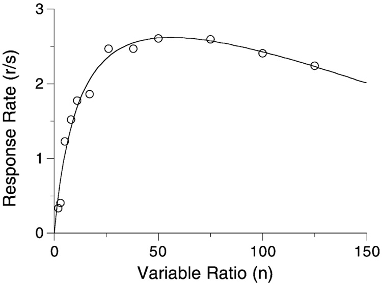
Fig. 15 shows the average data from four rats on a series of VR schedules whose mean is given on the x-axis. The curve is Eq. (4) with the coupling coefficient for VR schedules, Eq. (6).
Fig. 15.
Average response rates of four rats on a series of VR schedules. The curve comes from Eq. (4) and the coupling coefficient for VR schedules, with parameters δ = 0.25 s, β = 0.76, and a = 350 responses/reinforcer.
3. Realignments
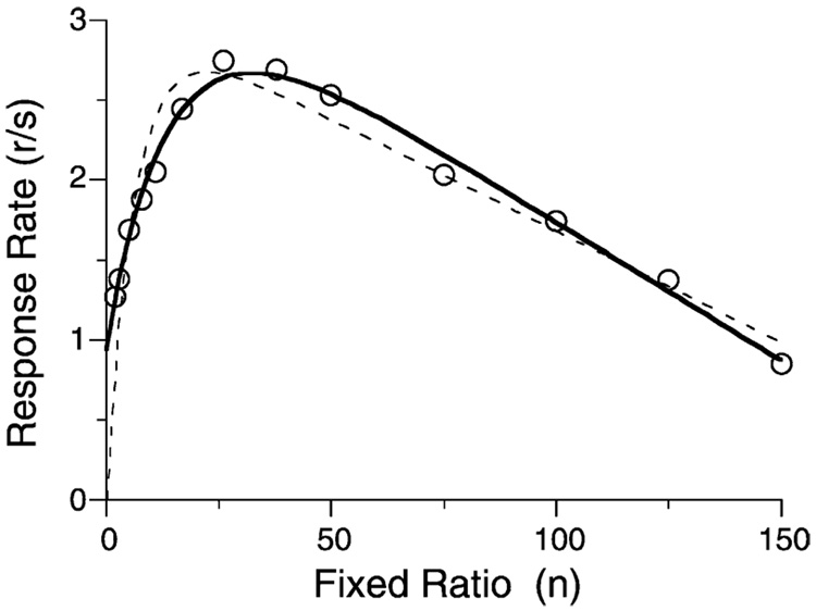
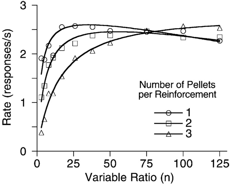
Model development proceeded in the simplest fashion consistent with the data; but then other data arose that were inconsistent with that development. Consider the FR data shown in Fig. 16. The first x-axis intercept of Eq. (5) is at 0, but these data start well above the x-axis. Eq. (5) predicts very low rates at small ratios due to the displacement of the memory of prior target responses by consummatory responses. This is shown by the dashed curve that Eq. (4) and Eq. (5) drawn through the data. Fig. 17 shows a more significant problem. In this experiment rats received either 1, 2, or 3 pellets for responding on VR schedules. Notice that for VRs of 3–50, one-pellet reinforcers generated significantly higher response rates than three pellet reinforcers. The story told by Fig. 17 is not simple: three pellets do sustain higher rates at the largest ratios. Control conditions ruled out satiation as the explanation of the impaired effectiveness of the larger reinforcers at small ratio values (Bizo et al., 2001).
Fig. 16.
Average response rates of four rats on a series of FR schedules. The curves are from Eq. (4) and the old coupling coefficient (dashed curve, Eq. (5)) or the new coefficient (continuous curve, Eq. (5′); parameters δ = 0.29 s, β = 0.25, and a = 200 responses/reinforcer).
Fig. 17.
Average response rates of five rats on a series of VR schedules. The curve comes from Eq. (4) and Eq. (6), with δ = 1/3 s, and β and a increasing with the number of pellets per reinforcement. From Bizo et al. (2001).
3.1. Incomplete erasure
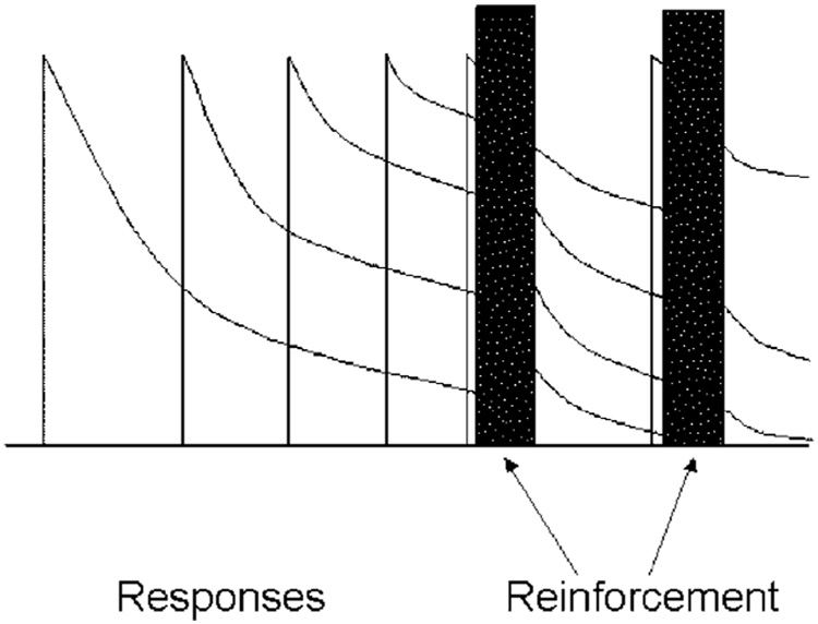
The problems displayed in both figures may be resolved by revisiting a simplifying assumption of the models for coupling, the one depicted in the reinforcement epoch of Fig. 13. Does reinforcement completely displace the traces of prior responses? This often seems to be the case for pigeons; but pigeons are typically given a relatively large amount of food as a reinforcer: around 1.4% of their daily requirement. A 45 mg food pellet is a significantly smaller portion of a rat’s daily requirement, and its consumption does not fill the 3 or 4 s that a pigeon reinforcer typically does. For generality, the coupling coefficient must be modified to allow for the possibility of a reinforcer strengthening not only immediately preceding responses, but also those that predated the prior reinforcer (see Fig. 18). For FR schedules it is simplest to add a free parameter n0 signifying the nominal number of additional responses beyond the prior reinforcer that contribute to response strength (the “savings”). The coupling coefficient for FR schedules becomes:
| (5′) |
Fig. 18.
The traces of early responses may bleed through a reinforcer to receive additional strengthening by a later reinforcer. The rapid attrition of the traces during reinforcement is due to the vigorous consummatory responses occurring then. Traces of these consummatory responses, and the focal search occurring immediately after them, are shown carried forward to the second reinforcement epoch as candidates for reinforcement.
In the rightmost part of the equation, epsilon (ε), which can range from 0 to 1, is the degree of erasure of memory for the target response exerted by the delivery and consumption of a reinforcer; ε = (1 − β)n0. If erasure is complete (ε = 1), there are no savings (n0 = 0) and Eq. (5) is recovered. The y-axis intercept is the response rate projected when n = 0. The FR model with Eq. (5′) as the coupling coefficient gives the intercept as y0 = (1−ε)/δ. With complete erasure, ε = 1, Eq. (5′) reduces to Eq. (5), with an intercept y0 = 0. As the savings n0 gets large, ε approaches zero and coupling approaches its maximum, 1.0. Thus with no erasure, which might be approximated by brief reinforcers such as brain stimulation or points added to a display, FR data fall along a decreasing straight line from y0 = 1/δ. With a value of n0 = 4 (ε = 0.75), Eq. (5′) draws the continuous curve shown in Fig. 16.
What of the paradoxical data shown in Fig. 17? The increased reinforcer magnitude does indeed increase specific activation a, and this is manifest in the shallower slope of the right tails of these functions. But it also increases the erasure of prior response traces. On variable ratio schedules, the effect of incomplete erasure is predicted to be an inflated value of β (Bizo et al., 2001; Eq. (6′)), not an elevation of y0. Eq. (3), using the basic coupling coefficient for VR schedules (Eq. (6)) as shown in the curves through the data in Fig. 17. No new parameters were necessary to fit the data, but the value assigned to the memory decay rate β was a confound of rate of decay and degree of erasure (ε). When erasure is included in the model, coupling is expressed as:
| (6′) |
Data can be accommodated without altering the decay rate, if that is set by other conditions. The rate of decay of response traces at three pellets—where erasure looked to be near complete—was β = 0.06 (half the value typically found for pigeons: Killeen and Fantino, 1990). If we assume erasure is complete (ε = 1) with three pellets, then ε = 0.37 for two pellets and ε = 0.17 for one pellet; a single pellet blocks the prior response traces from additional strengthening from subsequent reinforcers by only 17%.
3.2. Does the duration of a response (δ) affect the rate of decay of memory (β)?
Fig. 13 and Fig. 18 depict responses as instantaneous. Each response, no matter how long its duration, is weighted by β in memory and reduces the memory available to prior responses by the fraction 1 − β. But if responses extend over a period of time—if they comprise a sequence of motions each susceptible to reinforcement—then the weight of an event in memory should be the area of the trace decay that overlaps with reinforcement. For the response that triggered reinforcement, this area is 1 − e−λδ, where the parameter λ is the intrinsic rate of decay of memory (see Fig. 19). If responses are all of the same duration δ, then the formulations are essentially identical, with β = 1 − e−λδ. But if there is variation in response duration, whether within animals, across animals, or as a function of experimental manipulations, then the formulations make different predictions. A goal of modeling is to incorporate regularities of data into the structure of the model, rendering the parameters orthogonal. In an early formulation of MPR, no allowance was made for the duration of a response in calculating the rate of trace decay. When data from numerous studies were assembled, however, a strong positive correlation between β and δ (r = 0.8) was found. Within a single study, Bizo and Killeen (1997) changed the target response from key-pecking to treadle-pressing and found that β increased from 0.58 to 0.92. The parameters were being forced to do work that was not automatically being done by the model itself. Killeen (1994, Section 5.3.1) embedded the correlation in the model, conducting all further analyses under the assumption that β = 1 − e−λδ. Thus β, the proportion of allocation of memory to a target response, became a derived, rather than fundamental variable. Under this construction, the intrinsic rate of decay (λ) may be held constant in the Bizo and Killeen (1997) experiment, sacrificing less than 0.1% of the variance accounted for by the model.
Fig. 19.
Responses of extended duration occupy more of memory, and therefore increase the rate of decay.
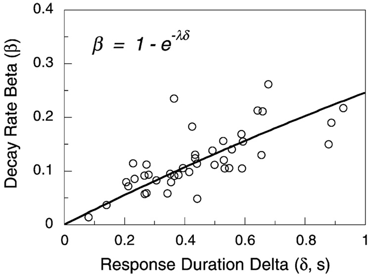
A nice demonstration that apparent rate of decay depends on response duration is found in a large-scale parametric study conducted by Reilly (2003), in which 42 rats were conditioned to respond on five-component multiple FR schedules. These data are valuable for examining the effect of individual differences in response topography, the determinant of δ. Eq. (4) with Eq. (5) as the coupling coefficient provided a good fit to the data—one identical to the old model (Eq. (4) and Eq. (5)). Fig. 20 is a scatter plot of the recovered values of β and δ for the old model. Their product-moment correlation is r = 0.72 (t = 6.56, P < 0.0001). When the correct representation is used, this correlation drops to a non-significant r = −0.18 (t = 1.13, P ≈ 0.2). There is no doubt that longer responses occupy— and displace—more memory than do brief responses. Where variation in response duration is not an issue, then the simple models—Eq. (5′) and Eq. (6′)—suffice. In conditions where response duration may vary, as under pharmacological manipulations, comparison of different populations, or even when reinforcement contingencies are varied, then the more complete model with 1 − e−λδ replacing β is recommended. Notice that making this substitution in Eq. (5′) yields three equivalent forms and an approximation:
| (5″) |
Fig. 20.
Eq. (4) and Eq. (5) fit to the data of 42 rats responding on multiple FR schedules yielded these recovered values of β and δ. Eq. (5″) incorporates this relation and orthogonalizes the parameters.
The first equation is the most transparent; the second the most compact; the third resonates with the founding intuitions; the last, valid when λδ ≫ 1, is most similar to Eq. (5′). When there is near-complete erasure (n0 ≈ 0), or for moderate and large ratios, then epsilon may vanish into 1. Notice that the first and second lines are equivalent because β = 1 − e−λδ. With a value of λ = 0.28 s−1, Eq. (5″) drew the curve in Fig. 20, accounting for half the variance in the data. The other half of the variance arises from differences among animals in the rate of trace decay (λ), along with measurement error. When variations in δ are a consideration for variable ratio schedules, 1 − e−λδ (or its approximation λδ) should replace β in Eq. (6). The closing forms of these equations are given in Table 2.
Table 2.
Fundamental equations
| Equation | Description | ||
|---|---|---|---|
| I | The fundamental equation of motion, combining the three basic principles of activation, constraint and direction; from Eq. (3) | ||
| II | Predicts response rates on ratio schedules; Eq. I with schedule feedback function for ratio schedules (r = b/n); from Eq. (4) | ||
| III | cFRn = 1 − εe−λδn | Coupling coefficient for fixed ratio schedules; from Eq. (5″) | |
| IV | Coupling coefficient for variable ratio schedules, in which: k = ε(eλδ − 1)−1; λ, δ > 0; from Eq. (6′) |
3.3. Does response duration (δ) affect the number of responses supported by a reinforcer (a)?
Skinner (1938) assumed that in extinction the rate of responding dB/dt decreased with each response withdrawn from the reserve: (A − kB); where k is a constant of proportionality, A the size of the reserve, and B the number of responses emitted (Killeen, 1988). This differential equation has a solution b = Ae−kt that is consistent with the exponential decay functions shown in Fig. 2. But those decay functions are also consistent with the assumption that responses of longer durations withdraw proportionately more from the reserve: b = A/δe−δt/k. In absence of the decisive data, Killeen (1994) assumed the latter, implementing the first principle as A = ar/δ. This led to a fundamental equation of motion slightly different from Eq. (3):
| (3′) |
The ensuing equation for ratio schedules was:
| (4′) |
The key difference between these original equations and the current versions (Eq. (3) and Eq. (4)) is that now the duration of a response δ multiplies a, whereas in the originals shown above it did not. Because a is a free parameter, the distinction makes no difference in the quality of fit between theory and data; it arises where variations in δ might confound the inferred value of specific activation.
Now the implementation of the first principle can be simplified in light of newer data. Reilly (2003) analyzed the lever-press rates of 42 rats responding on multiple schedules using Eq. (4′). If the new Eq. (4) is correct, there should be a positive correlation between 1/a and 1/δ in his recovered parameters. This is because the slope 1/a implied by Eq. (4′) omits the factor 1/δ found in Eq. (4). If Eq. (4) truly governs behavior, then when Eq. (4′) is fit to the data, 1/a must adjust to compensate for the omission of 1/δ. This will cause the recovered values of 1/a and 1/δ to be positively correlated. That is exactly what happened: the correlation between 1/a and 1/δ for Reilly’s data was r = 0.75 (t = 7.13, p < 0.0001). Use of Eq. (4) orthogonalizes the parameters: with it the correlation between 1/a and 1/δ falls to an insignificant r = 0.03. Skinner’s original (1938) intuition, in which response duration was not a factor in the depletion of the reserve, was after all correct.
4. Summary and conclusions
The basic principles of MPR have survived for a decade. This is not surprising, because they capture intuitions that are part of the tacit knowledge of the field:
4.1. A
Data such as those shown in Fig. 1 are not new: Fifty years ago Sheffield and Campbell noted that the effect of hunger “is to augment the normal activity responses to novel stimuli and to greatly augment the activity to stimuli associated with the performance of the consummatory response” (Sheffield and Campbell, 1954, p. 99). Nor is the use of a cumulative exponential to describe data like those in Fig. 2 new, although the curve was often misperceived to reflect learning rather than arousal (Hull, 1950; cf. Killeen, 1998). Here it is based on more primary data (Fig. 1) and an associated theory of accumulation (Fig. 4).
4.2. δ
Temporal constraints on response rate are so obvious as to have escaped comment. Yet they are at the heart of the concave relation between response rate and response probability (Killeen et al., 2002), and give Herrnstein’s hyperbola its form (Eq. (2); Staddon, 1977).
4.3. c
The effect of the contingency between responding and reinforcement on behavior—the law of effect—is the heart of the Skinnerian research program. Here the ploy is to embed this relation in a matrix that accounts for the first and second principles (Eq. (3)), partitioning the analysis by letting drive and incentive energize behavior, while contingencies direct it.
The modeling details that put the principles in contact with data continue to evolve. These adjustments do not discredit the principles so much as show that they are alive; the theory is an open architecture, able to be improved by any who will take time to master the operating system. For the convenience of those few, the fundamental equations discussed in this paper are listed in Table 2.
MPR has affinities with other theories of behavior, such as linear systems theory (McDowell et al., 1993), and momentum theory (Nevin, 2003). Both affinities shall be developed into formal relations in subsequent articles.
Acknowledgements
This research was supported by grants NSF IBN 9408022 and NIMH K05 MH01293.
References
- Baum WM. In search of the feedback function for variable-interval schedules. J. Exp. Anal. Beh. 1992;57:365–375. doi: 10.1901/jeab.1992.57-365. [DOI] [PMC free article] [PubMed] [Google Scholar]
- Baum WM. Performances on ratio and interval schedules of reinforcement: data and theory. J. Exp. Anal. Beh. 1993;59:245–264. doi: 10.1901/jeab.1993.59-245. [DOI] [PMC free article] [PubMed] [Google Scholar]
- Bharucha-Reid AT. Elements of the theory of Markov processes and their applications. New York: McGraw-Hill; 1960. [Google Scholar]
- Bizo LA, Kettle LC, Killeen PR. Rats don’t always respond faster for more food: the paradoxical incentive effect. Anim. Learn. Behav. 2001;29:66–78. [Google Scholar]
- Bizo LA, Killeen PR. Models of ratio schedule performance. J. Exp. Psychol.: Anim. Beh. Process. 1997;23:351–367. doi: 10.1037//0097-7403.23.3.351. [DOI] [PMC free article] [PubMed] [Google Scholar]
- Galbicka G, Platt JR. Parametric manipulation of interresponse-time contingency independent of reinforcement rate. J. Exp. Psychol.: Anim. Beh. Process. 1986;12:371–380. [PubMed] [Google Scholar]
- Herrnstein RJ. On the law of effect. J. Exp. Anal. Beh. 1970;13:243–266. doi: 10.1901/jeab.1970.13-243. [DOI] [PMC free article] [PubMed] [Google Scholar]
- Herrnstein RJ. Derivatives of matching. Psychol. Rev. 1979;86:486–495. [Google Scholar]
- Hull CL. Behavior postulates and corollaries-1949. Psychol. Rev. 1950;57:173–180. doi: 10.1037/h0062809. [DOI] [PubMed] [Google Scholar]
- Killeen PR. On the temporal control of behavior. Psychol. Rev. 1975;82:89–115. [Google Scholar]
- Killeen PR. Arousal: its genesis, modulation, and extinction. In: Zeiler MD, Harzem P, editors. Advances in Analysis of Behavior, Reinforcement and the Organization of Behavior. vol. 1. Chichester, UK: Wiley; 1979. pp. 31–78. [Google Scholar]
- Killeen PR. The reflex reserve. J. Exp. Anal. Beh. 1988;50:319–331. doi: 10.1901/jeab.1988.50-319. [DOI] [PMC free article] [PubMed] [Google Scholar]
- Killeen PR. Mechanics of the animate. J. Exp. Anal. Beh. 1992;57:429–463. doi: 10.1901/jeab.1992.57-429. [DOI] [PMC free article] [PubMed] [Google Scholar]
- Killeen PR. Mathematical principles of reinforcement. Behav. Brain Sci. 1994;17:105–172. [Google Scholar]
- Killeen PR. Economics, ecologics, and mechanics—the dynamics of responding under conditions of varying motivation. J. Exp. Anal. Beh. 1995;64:405–431. doi: 10.1901/jeab.1995.64-405. [DOI] [PMC free article] [PubMed] [Google Scholar]
- Killeen PR. The first principle of reinforcement. In: Wynne CDL, Staddon JER, editors. Models of Action: Mechanisms for Adaptive Behavior. Mahwah, NJ: Lawrence Erlbaum; 1998. pp. 127–156. [Google Scholar]
- Killeen PR. A passal of metaphors: “some old, some new, some borrowed …”. Behav. Brain Sci. 2000;23:102–103. [Google Scholar]
- Killeen PR. Writing and overwriting short-term memory. Psychol. Bull. Rev. 2001;8:18–43. doi: 10.3758/bf03196137. [DOI] [PMC free article] [PubMed] [Google Scholar]
- Killeen PR, Bizo LA. The mechanics of reinforcement. Psychol. Bull. Rev. 1998;5:221–238. [Google Scholar]
- Killeen PR, Fantino E. Unification of models for choice between delayed reinforcers. J. Exp. Anal. Beh. 1990;53:189–200. doi: 10.1901/jeab.1990.53-189. [DOI] [PMC free article] [PubMed] [Google Scholar]
- Killeen PR, Cate H, Tran T. Scaling pigeons’ choice of feeds: bigger is better. J. Exp. Anal. Beh. 1993;60:203–217. doi: 10.1901/jeab.1993.60-203. [DOI] [PMC free article] [PubMed] [Google Scholar]
- Killeen PR, Hall SS. The principal components of response strength. J. Exp. Anal. Beh. 2001;75:111–134. doi: 10.1901/jeab.2001.75-111. [DOI] [PMC free article] [PubMed] [Google Scholar]
- Killeen PR, Hall SS, Reilly MP, Kettle LC. Molecular analyses of the principal components of response strength. J. Exp. Anal. Beh. 2002;78 doi: 10.1901/jeab.2002.78-127. xx–yy. [DOI] [PMC free article] [PubMed] [Google Scholar]
- Killeen PR, Hanson SJ, Osborne SR. Arousal: its genesis and manifestation as response rate. Psychol. Rev. 1978;85:571–581. [PubMed] [Google Scholar]
- Killeen PR, Smith JP. Perception of contingency in conditioning: scalar timing, response bias, and the erasure of memory by reinforcement. J. Exp. Psychol.: Anim. Beh. Process. 1984;10:333–345. [Google Scholar]
- Lattal KA, Abreu-Rodrigues J. Memories and functional response units. Behav. Brain Sci. 1994;17:143–144. [Google Scholar]
- Lucas G, Timberlake W, Gawley DJ, Drew J. Anticipation of future food: suppression and facilitation of saccharine intake depending on the delay and type of future food. J. Exp. Psychol.: Anim. Beh. Process. 1990;16:169–177. [PubMed] [Google Scholar]
- McDowell JJ, Bass R, Kessel R. A new understanding of the foundation of linear system analysis and an extension to nonlinear cases. Psychol. Rev. 1993;100:407–419. [Google Scholar]
- McGill WJ, Gibbon J. The general-gamma distribution and reaction times. J. Math. Psychol. 1965;2:1–18. [Google Scholar]
- Nevin JA. An integrative model for the study of behavioral momentum. J. Exp. Anal. Beh. 1992;57:301–316. doi: 10.1901/jeab.1992.57-301. [DOI] [PMC free article] [PubMed] [Google Scholar]
- Nevin JA. Extension to multiple schedules: some surprising (and accurate) predictions. Behav. Brain Sci. 1994;17:145–146. [Google Scholar]
- Nevin JA. Measuring behavioral momentum. Behav. Process. 2002;57:187–198. doi: 10.1016/s0376-6357(02)00013-x. [DOI] [PubMed] [Google Scholar]
- Nevin JA. Momentum and A. Behav. Process. 2003 in press. [Google Scholar]
- Palya WL. Dynamics in the fine structure of schedule-controlled behavior. J. Exp. Anal. Beh. 1992;57:267–287. doi: 10.1901/jeab.1992.57-267. [DOI] [PMC free article] [PubMed] [Google Scholar]
- Reilly MP. Personal communication 2003 [Google Scholar]
- Sheffield FD, Campbell BA. The role of experience in the “spontaneous” activity of hungry rats. J. Comp. Physiol. Psychol. 1954;47:97–100. doi: 10.1037/h0059475. [DOI] [PubMed] [Google Scholar]
- Shettleworth SJ. Reinforcement and the organization of behavior in golden hamsters: hunger, environment, and food reinforcement. J. Exp. Psychol.: Anim. Behav. Process. 1975;1:56–87. [Google Scholar]
- Shull RL. Mathematical description of operant behavior: an introduction. In: Iversen IH, Lattal KA, editors. Experimental Analysis of Behavior. New York: Elsevier; 1991. pp. 243–282. [Google Scholar]
- Skinner BF. The Behavior of Organisms. New York: Appleton-Century-Crofts; 1938. [Google Scholar]
- Staddon JER. On Herrnstein’s equation and related forms. J. Exp. Anal. Beh. 1977;28:163–170. doi: 10.1901/jeab.1977.28-163. [DOI] [PMC free article] [PubMed] [Google Scholar]
- Timberlake W, Lucas GA. Behavior systems and learning: from misbehavior to general principles. In: Klein SB, Mowrer RR, editors. Contemporary Learning Theories: Instrumental Conditioning Theory and the Impact of Constraints on Learning. Mahwah, NJ: Lawrence Erlbaum; 1990. pp. 237–275. [Google Scholar]


