A neural code for three-dimensional object shape in macaque inferotemporal cortex

Abstract

Previous investigations of the neural code for complex object shape have focused on two-dimensional (2D) pattern representation. This might be the primary mode for object vision, based on simplicity and direct relation to the retinal image. In contrast, 3D shape representation requires higher-dimensional coding based on extensive computation. Here, for the first time, we provide evidence of an explicit neural code for complex 3D object shape. We used a novel evolutionary stimulus strategy and linear/nonlinear response models to characterize 3D shape responses in macaque monkey inferotemporal cortex (IT). We found widespread tuning for 3D spatial configurations of surface fragments characterized by their 3D orientations and joint principal curvatures. Configural representation of 3D shape could provide specific knowledge of object structure critical for guidance of complex physical interactions and evaluation of object functionality and utility.

A primary goal in the study of object vision is to decipher the neural code for complex object shape. At the retinal level, object shape is represented isomorphically (i.e., replicated point-for-point) across a 2D map comprising approximately 10⁶ pixels. This isomorphic representation is far too unwieldy and unstable (due to continual changes in object position and orientation) to be useful for object perception. The ventral pathway of visual cortex^1–2 must transform the isomorphic image into a compact, stable neural code that efficiently captures the shape information needed for identification and other aspects of object vision.

Previous studies of complex shape coding have focused on 2D pattern representation. These studies have shown that neurons at intermediate (areas V2 and V4) and final (IT) stages in the monkey ventral pathway process information about 2D shape fragments. V2 and V4 neurons encode curvature, orientation, and object-relative position of 2D object boundary fragments^3–7. At the population level, these signals combine to represent complete boundary shapes as spatial configurations of constituent fragments⁸. In posterior IT, individual neurons integrate information about multiple 2D boundary fragments, producing explicit signals for more complex shape configurations^9–10. In central/anterior IT, the homologue of high-level object vision regions in human cortex^11–13, neurons are selective for a variety of patterns and that selectivity is organized across the cortical surface in a columnar fashion^14–18. At each stage, neurons appear to be tuned for component-level shape, although holistic shape tuning can evolve in IT through learning¹⁹. Holistic object representation may be more fully realized in medial temporal brain structures associated with long-term declarative memory²⁰ and in prefrontal areas processing categorical object information²¹.

The question addressed here is whether and how complex 3D shape is encoded by IT neurons. Our specific hypothesis is that IT neurons encode 3D spatial configurations of surface fragments. Under this hypothesis, the 2D structural representations described above could be considered to occupy a subspace within the higher-dimensional 3D structure domain. (I.e., surface fragments forming the 2D self-occlusion boundary of an object would be a special case of 3D surface fragments.) This hypothesis is consistent with classic shape coding theories in which objects are represented as 3D spatial configurations of simple 3D parts^22,23. The alternative hypothesis, advanced in more current theories, is that complex shape perception is based primarily on 2D image processing. According to these theories, consistent recognition of 3D objects from different vantage points is achieved by learning associations between multiple 2D views²⁴. The multiple-views hypothesis avoids the time-consuming computational complexity of inferring 3D structure. This hypothesis is supported by psychophysical results showing that view-invariant recognition is learning-dependent^25,26 and by computational studies showing that 2D image processing can support rapid, accurate object identification^27,28. (However, these results and the multiple-views hypothesis itself are also compatible with 3D representation²⁹; see Discussion.)

The classic hypothesis that complex shapes are represented as 3D spatial configurations of 3D parts has yet to be tested at the neural level. Previous studies have shown differential responses across a small number of 3D shapes³⁰ or tuning along a single depth-related dimension^31–34, but such results cannot demonstrate or explain complex 3D shape representation. (Similar responses in dorsal pathway cortex have been interpreted as signals for orientation in depth³⁵.) Representation of 3D object shape would require neurons with much more complex, multidimensional tuning properties. That kind of tuning can only be measured with large stimulus sets in which a wide range of 3D shape elements are combined in many different ways, so that quantitative analyses can disambiguate which 3D shape factors (if any) are uniquely and consistently associated with neural responses. This has not been attempted before due to the intractable size of 3D shape space. In this virtually infinite domain, a conventional random or systematic (grid-based) stimulus approach can never produce sufficiently dense, combinatorial sampling.

We addressed this obstacle with a novel evolutionary stimulus strategy. Beginning with an initial generation of 50 random 3D shapes, stimuli evolved through multiple generations under the guidance of neural feedback. Ancestor stimuli from previous generations were probabilistically morphed, either locally or globally, to produce descendant stimuli that varied the ancestor’s shape characteristics and/or combined them with new shape features. The average neural response to each stimulus determined the probability with which it produced morphed descendants in subsequent stimulus generations. This strategy has two advantages. First, sampling becomes increasingly focused around the response range of the neuron, so that far less experimental time is spent sampling null response regions. Second, in the high-response stimulus lineages, the (initially unknown) shape characteristics encoded by the neuron are repeatedly varied and recombined with other shape features. The result is much denser, more combinatorial sampling in the most relevant region of the 3D shape domain. (In contrast, standard gradient descent search aims to identify a single, maximum response stimulus, which by itself cannot reveal what specific shape information is encoded by a neuron.) This evolutionary stimulus strategy made it possible for the first time to test the 3D configural coding hypothesis at the neural level.

RESULTS

Random 3D shape stimuli were constructed by extensively deforming a closed ellipsoidal surface (Supplementary Fig. 1 online). These stimuli were rendered in depth by a combination of binocular disparity and shading cues. Two rhesus monkeys were trained to maintain fixation on a small spot while stimuli were flashed for 750 ms each at the center of gaze. We recorded the stimulus responses of individual neurons in central and anterior IT (between 5.8 and 21.0 mm anterior to the interaural line). Neurons were typically tested with 8–10 generations of 50 stimuli each. When recording time permitted, the entire procedure was run a second time, to verify that stimulus evolution would converge in the same direction (Fig. 1, left and right columns). In each run, the initial generation was completely random, and responses were generally low (Fig. 1a).

Figure 1. Evolutionary 3D shape experiment.

Two independent stimulus lineages (Run 1 and Run 2) are shown in the left and right columns respectively. Background color (see scale bar) indicates the average response to each stimulus of a single IT neuron recorded from the ventral bank of the superior temporal sulcus (6.45 mm anterior to the interaural line). (a) Initial generations of 50 randomly constructed 3D shape stimuli. Stimuli are ordered from top left to bottom right according to average response strength. (b) Partial family trees showing how stimulus shape and response strength evolved across successive generations. (c) Highest response stimuli across 10 generations (500 stimuli) in each lineage. (d) Linear/nonlinear response models based on two Gaussian tuning functions. The Gaussian functions describe tuning for surface fragment geometry, defined in terms of curvature (principal, i.e. maximum and minimum, cross-sectional curvatures), orientation (of a surface normal vector, projected onto the x/y and y/z planes), and position (relative to object center of mass in x/y/z coordinates). The curvature scale is squashed to a range between –1 and 1 (see Methods). The 1.0 standard deviation boundaries of the two Gaussians (magenta and cyan) are shown projected onto different combinations of these dimensions. These boundaries appear circular because standard deviations in the curvature, orientation, and position dimensions were constrained (respectively) to have the same values in order to limit model complexity. The equations show the overall response models, with fitted weights for the two Gaussians, the product or interaction term, and the baseline response. (e) The two Gaussian functions are shown projected onto the surface of a high response stimulus from each run. The stimulus surface is tinted according to the tuning amplitude in the corresponding region of the model domain. In this and subsequent displays, the projection areas are extended to include strongly correlated surface regions (see Methods). The scatterplots show the relationship between observed responses and responses predicted by the model. In each case, self-prediction by the model is illustrated by the stimulus/scatterplot pair on the left and cross-prediction by the pair on the right.

Higher response stimuli had a greater probability of producing morphed descendants in subsequent generations, and response levels progressed across generations in a way that was sometimes gradual and sometimes punctuated (Fig. 1b; also see Supplementary Figs. 2, 3, 4 and 5 online). In any given generation, only a few descendants produced higher responses; most descendants evoked equivalent or lower responses. These lower response samples in neighboring shape space are essential for characterizing the shoulders and boundaries of tuning functions.

For this example cell, both lineages converged toward shapes that varied on the global level but contained consistent local structure comprising sharp protrusions and indentations, oriented toward the right and positioned to the upper right of object center (Fig. 1c). We quantified this response pattern with a multi-component model analogous to those applied recently to dorsal pathway area MT and in posterior IT cortex^{9–10, 36}. In the MT analyses, the model components represent tuning for different movement directions in the orientation domain. Here, the model components represent tuning for different surface fragments in a 3D curvature/orientation/position domain. The two tuning models based on the two runs for this neuron (Fig. 1d) both comprised two component Gaussian functions, denoted by magenta and cyan. The magenta functions are centered on strongly positive (convex) maximum curvature and negative (concave) minimum curvature, indicating a hyperbolic or saddle-shaped surface. This surface is oriented to the right (0°) and positioned to the upper right in the x/y plane. The cyan functions are centered on convex/convex curvature, oriented downwards (270°) and positioned to the upper right.

The predicted response for a given stimulus depended on how closely any of its constituent surface fragments matched these tuning functions. The overall predicted response was a linear combination of predictions based on the two separate functions plus a nonlinear interaction term (Fig. 1d, equations). In this case, the nonlinear interaction terms had the highest fitted weights, showing that neuron was relatively selective for the combination of both types of surface fragments. Higher response stimuli in both runs included surface fragments near these two Gaussian functions (Fig. 1e, magenta- and cyan-tinted surface regions). In this and all subsequent stimulus plots, the tinted regions include any additional surface structure strongly correlated with the Gaussian tuning function, to better capture the entire surface configuration associated with neural responses. This is necessary because the geometry of closed, continuous surfaces imposes strong local structure correlations. For example, sharp points (tangent discontinuities) are necessarily correlated with the conjoined surfaces that define them, as in Fig. 1e. From a mechanistic point of view, the neuron’s response could be driven by a sub-portion of that structure, but geometric constraints make that difficult or impossible to test in an experiment of this kind.

These tuning models showed strong cross-prediction of responses in the other run (r = 0.67 for run 1 model cross-prediction of run 2; r = 0.63 for run 2 model cross-prediction of run 1). The two runs provide a rigorous cross-validation test since they were generated completely independently. (Geometric similarities between runs are imposed by the neuron itself, and thus serve to confirm the generality of the tuning model.) Cross-validation analyses of all cells with double lineages (see Supplementary Fig. 6 online) established that models based on two Gaussian tuning regions had greater statistical validity than simpler models based on one Gaussian and more complex models based on three, four, or five Gaussians. Restricting models to subunits explaining at least 5% additional variance produced a corresponding predominance of 2-Gaussian models (see Supplementary Fig. 7 online). The results presented below are based on two-Gaussian models for 95 neurons that showed statistically significant cross-validation between two runs (n = 16) or 5-fold cross-validation within one run (n = 79). We corrected the 5-fold cross-validation procedure for standard error of the mean response measurements to estimate that these models accounted for 32% of the explainable response variance on average (mean r = 0.57; see Supplementary Fig. 6).

Fig. 1 exemplifies the expected pattern for cells that encode 2D boundary shape. Even though the response model domain encompasses 3D surface fragments, the fitting procedure finds surfaces at the 2D occlusion boundary, with normal orientations in the image plane, essentially corresponding to 2D boundary fragments. Correspondingly, control tests showed that this cell responded nearly as strongly to the same shapes when all depth cues were removed (producing a silhouette shape with no internal detail; Supplementary Fig. 8 online; 54 spikes s^-1 with stereo and shading cues, 44 spikes s^-1 without). However, this result did not typify the majority of neurons in our sample.

The more common finding was tuning for surface fragments outside the image plane, as in Fig. 2. The highest response shapes for this neuron were characterized by a ridge facing out of the image plane (Fig. 2a; also see Supplementary Fig. 9 online). Stimuli lacking this surface characteristic evoked little or no response (Fig. 2b). Control tests performed on stimuli drawn from the top, median, and bottom of the response range (Figs. 2c—h, top, middle, and bottom rows) confirmed that this neuron’s shape tuning was dependent on depth structure and robust to other image changes. The neuron remained responsive when either disparity or shading cues for depth were present but failed to respond when both were eliminated (Fig. 2c; see also Supplementary Fig. 10 online). 3D shape selectivity remained consistent across lighting directions over 180° vertical and horizontal ranges (Fig. 2d), in spite of the resulting dramatic changes in shading patterns across the object surface (Supplementary Fig. 11 online). Selectivity was likewise consistent across changes in stereoscopic depth (Fig. 2e) and x/y position (Fig. 2f), although not across changes in stimulus orientation (Fig. 2g). Selectivity was consistent across stimulus size (Fig. 2h). The response model (Fig. 2i) comprised tuning for forward-facing ridges in front (magenta) and upward-facing concavities near object center (cyan). The model for this neuron was highly nonlinear, as shown by the large AB interaction term representing combined energy in the two tuning regions. Thus, this neuron provided a relatively explicit signal for the ridge/concavity configuration. (By “explicit”, we mean having a simple, easily decoded relationship to the shape configuration in question. Linear integration of information about multiple fragments would produce more ambiguous, less explicit signals, in which the same response level could correspond to either part A or part B.) This configuration characterized the high response stimuli in the evolutionary test (Fig. 2j; one high response stimulus is shown from both the front and above for greater visibility of the two surface components; see also Supplementary Fig. 12 online).

Figure 2. Neural tuning for 3D configuration of surface fragments.

Error bars indicate s.e.m. (a) Top 50 stimuli across 8 generations (400 stimuli) for a single IT neuron recorded from the ventral bank of the superior temporal sulcus (17.5 mm anterior to the interaural line). (b) Bottom 50 stimuli for the same cell. (c) Responses to highly effective (top), moderately effective (middle) and ineffective (bottom) example stimuli as a function of depth cues (shading, disparity, and texture gradients, exemplified in Supplementary Fig. 10 online). Responses remained strong as long as disparity (black, green, blue) or shading (gray) cues were present. The cell did not respond to stimuli with only texture cues (pale green) or silhouettes with no depth cues (pale blue). (d) Response consistency across lighting direction. The implicit direction of a point source at infinity was varied across 180° in the horizontal (left to right, black curve) and vertical (below to above, green curve) directions, creating very different 2D shading patterns (Supplementary Fig. 11). (e) Response consistency across stereoscopic depth. In the main experiment, the depth of each stimulus was adjusted so that the disparity of the surface point at fixation was 0 (i.e. the animal was fixating in depth on the object surface). In this test, the disparity of this surface point was varied from −4.5° (near) to 5.6° (far). (f) Response consistency across x/y position. Position was varied in increments of 4.5° of visual angle across a range of 13.5° in both directions. (g) Sensitivity to stimulus orientation. Like all neurons in our sample, this cell was highly sensitive to stimulus orientation, although it showed broad tolerance (about 90°) to rotation about the z axis (rotation in the image plane, blue curve); this rotation tolerance is also apparent among the top 50 stimuli in (a). Rotation out of the image plane, about the x axis (black) or y axis (green) strongly suppressed responses. (h) Response consistency across object size over a range from half to twice the original stimulus. (i) Linear/nonlinear response model based on two Gaussian tuning functions. Details as in Fig. 2d,e. (j) The tuning functions are projected onto the surface of a high response stimulus, seen from the observer’s viewpoint (left) and from above (right).

Tuning for 3D surface configurations (as in Fig. 2) was more common in our sample than tuning for 2D boundary configurations (as in Fig. 1). This was established by follow-up control tests measuring how responses depended on the presence of 3D cues (as in Fig. 2c). The critical comparison from these tests is between the condition in which the standard 3D cues (disparity and shading) were present and the condition in which no 3D cues were present, so that the stimulus was a plain 2D silhouette. In each condition, strength of modulation was measured by the response difference between a stimulus drawn from the top of the main test response range and a stimulus drawn from the bottom of the range, normalized by the maximum response across all conditions. Response modulation was generally strong (near 1.0) when 3D depth cues were present (Fig. 3a, horizontal axes). When depth cues were removed (vertical axes) modulation sometimes remained strong (points near the upper right), indicating that responses were based on 2D boundary shape. More commonly, however, modulation dropped to near 0, reflecting sensitivity to 3D shape. The drop in response modulation with removal of 3D cues does not simply reflect selectivity for 2D shading patterns, since 3D shape tuning was robust to changes in shading pattern produced by different lighting directions. We quantified this by measuring the separability of tuning for shape and tuning for lighting direction (Fig. 3b). 3D shape responses were likewise robust to changes in x/y position, stereoscopic depth and stimulus size (Fig. 3b), analogous to previous results showing similar tolerance in 2D shape responses³⁷.

Figure 3. Prevalence of 3D shape tuning in IT.

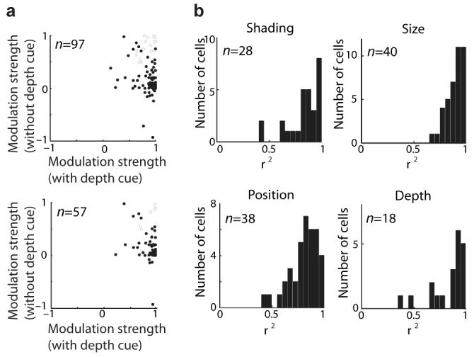
(a) Response modulation depended strongly on 3D cues for the majority of neurons in our sample. For each cell, three stimuli (with high, medium, and low responses in the evolutionary test) were presented with depth cues (disparity and shading) and without (solid color silhouette stimuli with the same boundary shape). A separate modulation index (difference between maximum and minimum responses, normalized by maximum response across the entire test) was calculated for the with- and without-depth cue conditions. The modulation index is the response difference between the high- and low-response stimuli, normalized by maximum response across all conditions. This normalization ensures that high values reflect robust responses. In some cases, removing 3D cues reversed the rank order of responses and produced negative index values. The average modulation index of 0.85 with depth cues (horizontal axis) dropped to 0.26 without depth cues. The effect of depth cues on responses was significant (P < 0.05) for 76/97 cells (filled circles) based on two-way ANOVA (main or interaction effects of stereo and shading). Of the 95 cells with significant 3D shape tuning models, 57 were tested in this way. For these cells, the modulation index average dropped from 0.87 with depth cues to 0.23 without, and the 49/57 cells showed significant main or interaction ANOVA effects. (b) Shape tuning was independent of shading pattern, stereoscopic depth, stimulus position and stimulus size. Response consistency across these factors was tested as shown in Fig. 2. Response consistency was measured by separability of tuning for shape (across the high, medium, and low response stimuli) and tuning for shading, depth, position, or size. Separability is represented here by the fraction of response variance (r²) explainable by a matrix product between separate tuning functions for shape and shading/depth/position/size. These tuning functions were the first pair of singular vectors in a singular value decomposition of the observed tuning matrix. For each factor, most neurons have r² values above 0.75, showing that 3D shape tuning is largely independent of lighting direction, stimulus position, stimulus size, and stimulus depth.

Tuning models spanned a wide range of surface fragment configurations (Fig. 4a,b). Component fragments were frequently discontiguous, consistent with a multi-fragment configural coding scheme. Even when tuning regions were extended to cover structures strongly correlated with the fitted Gaussians (as in Fig. 4), only a fraction (on average 23%) of total object surface area was included (Supplementary Fig. 13 online). Correspondingly, the global shape of high response stimuli varied at locations outside these surface regions. Thus, 3D shape representation in IT is not generally holistic. IT neurons represent spatially discrete 3D shape components, and must cooperate in a distributed coding scheme.

Figure 4. 3D surface configuration tuning patterns.

(a) All neurons for which two independent evolutionary stimulus lineages were obtained. In each case, two high response stimuli are shown from the first run (top row) and the second run (bottom row). Best fit 2-component models are projected onto these stimuli as in Fig. 1e. (b) Example neurons for which only one lineage was obtained. In each case, two high response stimuli are shown with the best fit model projected onto the surface.

Tuning models showed a predictable bias toward surface positions near the front of the object, which is more visible and behaviorally relevant under normal circumstances (Fig. 5a,b). Tuning was markedly biased in the curvature domain toward high values, especially on the convex end of the scale. Thus, although object surface area is dominated by flat or broad curvature (Fig. 5c), the IT representation of 3D shape emphasizes sharper projecting points and ridges (Fig 5d). Tuning for non-zero curvature reflects the coding advantage of higher order derivatives³⁸. The bias toward convexity may reflect the functional importance of protruding object parts and/or the well-established perceptual bias toward interpreting convexities as objects parts and concavities as junctions between parts³⁹.

Figure 5. Distribution of 3D shape tuning.

(a) Comparison distribution of surface point positions in the y/z plane (relative to object center of mass) in random stimuli (1^st generation stimuli for all 95 neurons described here). The scale is in arbitrary units approximately corresponding to stimulus size (maximum span in any direction averaged across stimuli = 1.08). (b) Distribution of Gaussian tuning peaks in best-fit models for 95 neurons. The stimulus distribution peak is shown in the surface plot (asterisk) and the stimulus distributions are shown in the marginal histograms (red curves). The distribution is biased toward positive values in the z dimension, i.e. positions in front of object center. (c) Comparison distribution of surface curvatures across random (1^st generation) stimuli. The bias toward positive (convex) curvatures is characteristic of closed, topologically spherical surfaces. (d) Distribution of Gaussian tuning peaks in the curvature domain. The stimulus distribution peak is shown in the surface plot (asterisk) and the stimulus distributions are shown in the marginal histograms (red curves). Relative to the stimulus distribution, the tuning peaks are biased toward higher magnitude convexity in the maximum curvature dimension and higher magnitude concavity in the minimum curvature dimension.

DISCUSSION

We tested the classic hypothesis that complex shapes are represented as 3D spatial configurations of 3D parts. This hypothesis requires that neurons encode the 3D shape, 3D orientation, and relative 3D position of object parts. Our analyses show that a substantial fraction of IT neurons do exactly that—they are simultaneously tuned for 3D shape (maximum and minimum principle surface curvatures), 3D orientation, and relative 3D position of constituent surface fragments. Moreover, they are tuned for multiple regions in this domain, i.e. they respond to shapes that include a specific configuration of particular surface features. This result supports classic theories of 3D configural shape representation^22,23, and extends those theories by suggesting that neurons encode not just individual parts but configural relationships between multiple parts.

In many cases, our analyses and follow-up control tests revealed exclusive tuning for 2D boundary shape. The majority of neurons in our sample, however, were clearly tuned for 3D spatial configurations of 3D surface fragments. Our control tests eliminate explanations based on other stimulus properties besides 3D shape. For example, neural responses might have been associated with 2D boundary shape features, since these can be strongly correlated with 3D surface shape⁴⁰. But our depth cue test showed that, for most cells, removing 3D information and presenting only the 2D boundary resulted in a drastic loss of tuning/responsiveness (Fig. 3a). Alternatively, neural responses might have been associated with the 2D shading patterns we used to help convey 3D shape. But our lighting direction test showed that dramatic changes in the 2D shading pattern (Supplementary Fig. 11) had little effect on shape tuning (Fig. 3b). Neural response differences might have reflected tuning for binocular disparity, but our depth position test showed that large changes in disparity had little effect on tuning (Fig. 3b). These three control tests eliminate alternate explanations based on any stimulus characteristic associated with the 2D boundary, 2D shading pattern, or disparity values, and these three elements constitute all the image information present in these stimuli. Likewise, large changes in stimulus size and position typically had little effect on tuning (Fig. 3b). No other potentially explanatory stimulus properties apart from 3D surface shape itself would have survived all these major image changes. As a further control, we performed an analysis to show that response variations could not be explained in terms of image spatial frequency content (Supplementary Fig. 6).

Our results are largely consistent with classic theories of configural shape representation^22,23. According to these theories, objects are represented as spatial configurations of canonical 3D parts. The parts are generalized cones or more complex volumetric components called “geons”. Their configuration is represented in an object-defined reference frame that translates, scales, and rotates with the object (producing invariance to viewpoint). Correspondingly, we observed explicit signals for configurations of 3D surface fragments that appear to be encoded in an object-relative 3D reference frame. By “explicit”, we mean easily decoded signals with clear, simple relationships to large-scale 3D object structure. In contrast, although the same information is necessarily present in V1 (from which IT responses ultimately derive), the V1 representation is highly implicit and difficult to decode, because it is distributed across a much larger population of neurons with complex, highly variable relationships to large-scale 3D object structure.

However, our results differed in two ways from classic theories. First, while the neural reference frame appeared to translate and scale with the object (given the consistency of responses across stimulus position and size) we did not find any evidence that it rotates with the object. Generalization across object rotations may depend on learned associations between views^24,41, although there is some capacity for recognizing rotated views of novel objects⁴². Representation of 3D structure is not incompatible with that view²⁹. Second, classic theories envision that individual neurons would represent single, spatially discrete parts. Instead, consistent with our previous 2D studies, we found that neurons represent configurations of multiple parts, frequently at distant, discontiguous locations on the object surface (Supplementary Fig. 14 online). Integration across multiple boundary and surface regions to derive larger, more complex configurations may be a ubiquitous aspect of visual processing⁴³. Complete 3D shapes might be represented in terms of a small number of component surface configurations (Fig. 6). A coding scheme like this still has the combinatorial productivity of parts-based representation—a finite number of signals can be combined in many different ways to represent a virtual infinity of objects. At the same time, it would constitute a step toward holistic shape coding, which has greater potential for sparseness. A sparse object representation based on just a few signals can be more efficiently stored in memory and decoded by other parts of the brain^44,45. The configural coding we observe may reflect a compromise between productivity and sparseness in higher-level visual cortex.

Figure 6. Configural coding of 3D object structure.

To illustrate how complex 3D shape could be encoded at the population level, five 2-Gaussian tuning models (red, green, blue, cyan, magenta) from our neural sample are projected onto a 3D rendering (right) of the larger figure in Henry Moore’s “Sheep Piece” (1971-72, left; reproduced by permission of the Henry Moore Foundation, www.henry-moore-fdn.co.uk). (Tuning models were scaled and rotated to optimize correspondence.) A small number of neurons representing surface fragment configurations would uniquely specify an arbitrary 3D shape of this kind and would carry the structural information required for judging its physical properties, functionality (or lack thereof), and aesthetic value.

The neural code we observed here is a 3D generalization of the 2D coding scheme we have previously described^8–9. Boundary fragments in 2D generalize to surface fragments in 3D. The circular orientation domain for 2D boundary fragments in the image plane generalizes to the spherical orientation domain for 3D surface fragments. Tuning for 2D boundary fragment curvature generalizes to joint tuning for the two principal curvatures characterizing any 3D surface fragment. Tuning for relative position of boundary fragments in the 2D image plane generalizes to tuning for relative position of surface fragments in 3D space. Conceivably, the 2D shape tuning properties that we and others have studied previously are not in any way distinct, and simply occupy a subspace in the higher dimensional 3D domain. In other words, neurons tuned for 2D shape might simply be a subpopulation (within a 3D shape representation) encoding surface fragments near the occlusion boundary. The predominance of 3D shape sensitivity in our neural sample supports this suggestion. However, this bias might be due to denser sampling in the superior temporal sulcus, which has been reported to contain more 3D-sensitive neurons⁴⁶ (see Supplementary Fig. 15 online).

To summarize, we used a novel evolutionary stimulus strategy to reveal for the first time an explicit structural code for 3D object shape in high level visual cortex. This code is embodied by neurons tuned for configurations of multiple object surface fragments. This result rules out the alternative that complex shape representation is primarily 2D, as in most current computational models of object vision. It supports classic theories of 3D structural representation^22,23, but qualifies those theories in two ways. First, individual neurons represent not single object parts but configurations of multiple object parts, providing more explicit signals for spatial relationships between shape elements. Second, the spatial reference frame is only partially defined by the object. The reference frame is centered with respect to the object, but contrary to classic theories does not rotate with the object. Thus, neural representations are very different depending on viewpoint, and relationships between different views of the same object would have to be learned, as proposed in view-dependent theories of object representation^24–26. Finally, these results apply only to the population of neurons we were able to study effectively with our stimulus strategy, and they do not rule out other object processing mechanisms in other neural populations. In particular, rapid, coarse object categorization might depend on faster, feedforward processing of 2D image information²⁸.

Why would the brain explicitly represent complex 3D object shape, considering the computational expense of inferring 3D structure from the 2D retinal image and the higher neural tuning dimensionality required? In contrast, 2D shape representations are lower-dimensional and can be derived quickly and directly from the retinal image. Moreover, computational studies of biologically-inspired hierarchical network models show that 2D image processing alone can produce rapid, accurate object identification^27,28. We speculate that representation of 3D object structure instead supports other aspects of object vision beyond identification. Direct cognitive access to 3D object structure makes even unfamiliar objects comprehensible in terms of their geometric similarity to familiar objects, inferred physical properties, potential functionality and utility, and aesthetic qualities. Knowledge of 3D structure is also necessary for accurate prediction of physical events and control over complex physical interactions with objects. These cognitive and behavioral requirements may have driven the emergence of an explicit neural code for 3D object structure in visual cortex. Similar tuning might emerge from hierarchical network models given 3D input information and more diverse task demands.

METHODS

Behavioral task

Two head-restrained rhesus monkeys (Macaca mulatta), a 9.5 kg male and a 5.3 kg female, were required to maintain fixation on a 0.1° spot within a 0.75° radius for 4 s in order to obtain a juice reward. Eye position was monitored with an infrared eye tracker (ISCAN). Separate left and right eye images were presented via mirrors. Binocular fusion was verified with a random dot stereogram search task. All animal procedures were approved by the Johns Hopkins Animal Care and Use Committee and conformed to National Institutes of Health and US Department of Agriculture guidelines.

Electrophysiological recording

The electrical activity of well-isolated single neurons was recorded with epoxy-coated tungsten electrodes (A-M Systems) and amplified and filtered in a Tucker-Davis Technologies acquisition system. We studied 250 neurons with at least 300 stimuli. Of these, 95 (59 from the male, 36 from the female) produced models that passed our statistical thresholds (Results). These neurons were sampled from the central/anterior lower bank of the superior temporal sulcus and lateral convexity of the inferior temporal gyrus (5.8–21.0 mm anterior to the interaural line; see Supplementary Fig. 15). IT cortex was identified based on structural MRI images.

Visual stimuli

3D shape stimuli were rendered with shading and binocular disparity cues using the NURBS facility in OpenGL (gluNurbsSurface). NURBS control point positions were varied by distorting a polar grid (see Supplementary Fig. 1). Stimulus depth was adjusted so that the depth of the object surface at the fovea matched fixation depth (screen distance).

Neurophysiological testing protocol

A roughly optimal stimulus color (white, red, green, blue, cyan, yellow, or magenta) was selected based on responses to stimuli under experimenter control. During all subsequent tests, following initiation of fixation, four stimuli were flashed one at a time for 750 ms each, with inter-stimulus intervals of 250 ms. Control tests of sensitivity to depth cues, x/y position, stereoscopic depth, size, orientation, and lighting direction (see Fig. 2) were performed on three stimuli, drawn from the top, median, and bottom of the response range in the main experiment.

Evolutionary morphing algorithm

The first stimulus generation contained only randomly generated 3D stimuli. Stimulus responses (averaged across 5 repetitions) were ranked into 10 bins with equal numbers of stimuli. In the second generation, 10–20% of stimuli were randomly generated. The rest were morphed descendants of ancestor stimuli from the first generation, selected randomly in equal numbers from the 10 bins. Thus, a typical second generation would contain 10 stimuli generated de novo, 4 descendants of stimuli in the highest response bin, 4 descendants from the second highest bin, etc. In subsequent generations, ancestor stimuli were pooled across all preceding generations and re-binned. Descendant stimuli had an equal probability of being either locally or globally morphed (see Supplementary Fig. 1). The amplitude of control point changes was inversely proportional to response rate, to produce denser sampling in higher response ranges.

3D shape response models

We characterized each 3D stimulus in terms of its component surface fragments. The stimulus surface was densely sampled across the NURBS control point grid. At each point, 7 values were determined: x, y, and z positions, relative to stimulus center of mass, surface normal orientation on the x/y and y/z planes, and maximum and minimum (principal) cross-sectional curvatures, squashed to a range from −1 to 1 using a sigmoidal function. Component surface fragments were defined by mathematically fitting elliptical regions on this grid with approximately constant curvature in either the minimum or maximum curvature dimensions. Each ellipse was shifted and scaled to be as large (i.e. cover as many grid points) as possible without violating constraints on maximum deviation of curvature values. Successive ellipses were fitted to remaining regions on the object surface. Curvature maxima and minima were also used to define surface fragments. On average, a given stimulus comprised 240 component surface fragments. For each fragment, maximum and minimum curvature were averaged across the included surface points, and the position and orientation values were measured at the point of maximum or minimum curvature, yielding 7 measurements. Thus, each fragment corresponded to a point in a 7-dimensional domain, and each stimulus was represented by a constellation of such points. All the models described here were based on 7D Gaussian tuning functions (model subunits) in this domain. The predicted response component due to a given subunit was based on the Gaussian function amplitude at the stimulus point closest to the Gaussian peak:

$$\begin{array}{cc}\hfill & \mathrm{Re}{\text{sponse}}_{\text{subunit}}=A\cdot \max \left(\text{Gaussian}\left(k{a}_{c}k{b}_c\theta x_c\theta y_{c}r{x}_{c}r{y}_{c}r{z}_c\right)\right)\hfill \\ \hfill & \text{Gaussian}\left(k{a}_{c}k{b}_c\theta x_c\theta y_{c}r{x}_{c}r{y}_{c}r{z}_c\right)=-\exp (\frac{{(k{a}_c-{\mu }_{ka})}^2}{2{\sigma }_k^2}+\frac{{(k{b}_c-{\mu }_{kb})}^2}{2{\sigma }_k^2}+\frac{{(\theta x_c-{\mu }_{\theta x})}^2}{2{\sigma }_{\theta }^2}+\frac{{(\theta y_c-{\mu }_{\theta y})}^2}{2{\sigma }_{\theta }^2}+\hfill \\ \hfill & +\frac{{(r{x}_c-{\mu }_{rx})}^2}{2{\sigma }_r^2}+\frac{{(r{y}_c-{\mu }_{ry})}^2}{2{\sigma }_r^2}+\frac{{(r{z}_c-{\mu }_{rz})}^2}{2{\sigma }_r^2})\hfill \end{array}$$

where ka_c, kb_c, Θx_c, Θy_c, rx_c, ry_c, and rz_c are the curvature, normal, and relative position values for a surface fragment in the stimulus, μ and σ are the fitted Gaussian peaks and the standard deviations on each of these seven dimensions, and A is the fitted Gaussian amplitude. The standard deviations in the curvature, orientation, and position dimensions were constrained to be the same (respectively) for all Gaussian functions in order to limit model complexity (i.e. only 3 standard deviation values were required for any given model, one each in the curvature, orientation and position dimensions). Including separate standard deviation parameters for each dimension slightly increased variance explained, by a mean of 3.7% for the 1-Gaussian models and 4.5% for the 2-Gaussian models (5-fold cross-validation, n = 95). Since the difference in explained variance between 1- and 2-Gaussian models increases, this would not impact our conclusion that neurons are tuned for configurations of multiple surface fragments rather than single fragments. The analyses presented here are based on the models with just 3 standard deviation parameters.

For each cell, we fitted models based on combinations of 1–5 excitatory Gaussian subunits. The predicted response to each stimulus was a weighted combination of the individual subunit responses (the linear component) and a product of subunit responses (the nonlinear interaction component). All possible combinations of subunits for nonlinear components were tested, but in the final models each subunit could participate in only one nonlinear interaction term. For the 2-Gaussian models emphasized in this report, there was only one possible interaction term.

$$\mathrm{Re}\text{sponse}=G\cdot \left(\sum _{s=1}^{\#\text{subunits}}\left(W_s{R}_s\right)+\sum _{k=1}^{\#\text{NLterms}}\left(W_k{R}_k^{NL}\right)\right)+b_0$$

where R_s is the unweighted response predicted by each subunit (derived from equation 1) and R^NL_s is the unweighted response predicted by each interaction term. W_s is the fitted weight (amplitude) for each subunit, W_k is the fitted weight for each interaction term, G is the overall gain, and b₀ is the baseline firing rate. The total numbers of fitted parameters for the models with 1–5 subunits were 13, 21–22, 29–30, 37–39, and 45–47, respectively. The variability in parameter number for higher order models is due to variability in the number of possible interaction terms. Overfitting was controlled by cross-validation analyses described in Results and presented in detail in Supplementary Fig. 6.

Response rates were calculated by counting the number of spikes during the 750-ms stimulus presentation period and averaged across repetitions. The Matlab function lsqnonlin was used to adjust model parameters to minimize the sum of squared differences between observed and predicted responses. The fitting procedure was repeated using 20–163 (average 93) starting points based on the constituent surface fragments for the 3 highest response stimuli. For each neuron, the best-fitting model across all starting points was used.

In some cases, these Gaussian tuning models may fail to capture the complete shape configurations associated with neural responses, instead focusing on smaller surface fragments within the complete configurations. This problem is inevitable due to the local surface structure correlations in any closed, continuous surface (Results). To better capture the complete shape configurations signaled by the neurons, we identified additional surface structure components that were highly correlated with those identified by the fitted Gaussian tuning regions. We then extended the tuning regions to include those correlated structures, up to the point at which explained variance dropped by 5%. The extended tuning regions are bound to have a non-Gaussian shape, which we approximated with a cluster of neighboring Gaussians. Predicted responses were based on average stimulus matches across the Gaussians in each cluster. These extended models were the basis for projections onto stimulus surfaces (Figs. 1e, 2j, and 4), tuning distributions (Fig. 5, Supplementary Figs. 16 and 17), and analysis of fractional surface coverage (Supplementary Fig. 12). All goodness of fit results were based on the original fitted 2-Gaussian models. The computational procedure for extending tuning regions is described in Supplementary Information (see Supplementary Fig. 13).

Statistical analysis

Randomization analysis of cross-validation between double lineages was used to compare the statistical validity of models based on 1–5 Gaussian tuning regions (see Supplementary Fig. 6). A 5-fold cross-validation procedure was used to estimate explained variance without overfitting (Results).