Statistical Analysis of Lateral Diffusion and Multistate Kinetics in Single-Molecule Imaging

Abstract

Single-molecule trajectories of molecules on the membrane of living cells have indicated the possibility that the lateral mobility of individual molecules is variable with time. Such temporal variation in mobility may indicate intrinsic kinetics of multiple molecular states. To clarify the mechanisms of signal processing on the membrane, quantitative characterizations of such temporal variations are necessary. Here we propose a method to analyze and characterize the multiple states in lateral mobility and their transition kinetics from single-molecule trajectories based on a displacement probability density function and an autocorrelation function of squared displacements. We performed our method for three cases: a molecule with a single diffusion coefficient (D), a mixture of molecules in two states with different D-values, and a molecule switching between two states with different D-values. Our analysis of numerically generated trajectories successfully distinguished the three cases and estimated the characteristic parameters for mobility and the kinetics of state transitions. This method is applicable to single-molecule tracking analysis of molecules in multiple functional states with different lateral mobility on the membrane of living cells.

Introduction

Signal transduction systems in living cells can be regarded as processes that regulate transitions between multiple states of signaling molecules. During transmembrane signaling, for example, receptors can adopt ligand-bound or -unbound states. Increasing the extracellular ligand concentration promotes the transition from unbound to bound states, which may enhance interactions with adaptor proteins in the intracellular surface, leading to an accumulation of receptors in the adaptor-bound state. Thus, to understand the mechanism of transmembrane signaling, it is imperative to determine how the state transition is regulated in time and space on the membrane of living cells.

For the study of such molecular state transitions in intracellular signal transduction, a molecule's lateral mobility is of particular importance because in certain cases it can be correlated to the molecular state as well as to the environmental conditions. For example, intermolecular interactions are thought to cause a decrease in diffusive mobility along the membrane (1–4). The interaction with the membrane's microdomain or cytoskeleton should also affect mobility (5–7). Furthermore, the diffusive properties of membrane molecules are not only important as an indicator of molecular states; they also act as a spatiotemporal control of signal transduction processes on the membrane. For signaling molecules, such as receptors, mobility may affect the retention of environmental cues on the membrane (8). Diffusive properties also control spatiotemporal patterns formed by self-organization processes, such as Turing patterns (9). Therefore, it is quite important to measure the diffusive properties of signaling molecules to study the spatiotemporal coordination of cellular processes.

Lateral diffusive mobility on the membranes of living cells has been measured by several means (10,11). For example, fluorescent recovery after photobleaching is a well-established technique in which the exchange of molecules can be monitored by discerning subpopulations by fluorophore photobleaching (12,13). Alternatively, fluorescence correlation spectroscopy measures both diffusion coefficients and concentrations of fluorescent molecules by detecting fluctuations in fluorescent intensity in a small volume (14). However, since these methods provide only ensemble-averaged information regarding the subpopulations, it is impossible to determine the transition kinetics of diffusion mobility. On the other hand, single-molecule imaging and tracking can potentially provide the needed temporal information (15).

Methods that are commonly used for mobility analysis of individual molecules utilize the mean-square displacement (MSD) calculated from each trajectory of the molecules (16,17). In the case of simple diffusion on a two-dimensional plane, the time evolution of the MSD ideally follows 4Dt. The advantage of this method is that it detects anomalous diffusion, such as diffusion in confined areas or with directed flows such that the time evolution of the MSD will display some deviation from 4Dt (18,19). In fact, previous studies using single-molecule tracking of membrane proteins have successfully shown constrained diffusion due to the membrane cytoskeleton and compartments on the membrane (20,21). However, the MSD has limitations when applied to diffusion coefficient estimation (17). Since the whole time duration of the trajectories is finite and thus the individual MSD plots naturally contain some fluctuation around 4Dt, the estimated diffusion coefficients obey some probability distribution function. The distribution obtained from these trajectories with ideally long durations shows a Gaussian-like distribution; however, a short time duration leads to an asymmetrical distribution, with the peak value of the distribution deviating from the true diffusion coefficient value (see Appendix SA in the Supporting Material). Because the exact distribution function is unknown, the MSD method is inadequate for describing the diffusion properties of molecules. This limitation is prominent when the molecule exhibits multiple states with different mobilities, where it is more difficult to estimate multiple diffusion coefficients. Furthermore, when the molecule shows state transitions, the state transition rates, as well as the diffusion coefficients, cannot be determined quantitatively. In addition, MSD analysis sometimes overlooks state transitions in mobility (Appendix SA in the Supporting Material). Thus, to reveal temporal variability in the mobility of molecules moving on the membrane, a new method to quantitatively describe mobility and the kinetics of the temporal changes of single-molecule trajectories is needed.

In this study, we propose a theory and a method for the kinetic analysis of temporal changes in the lateral mobility of single molecules on a membrane. To describe lateral mobility with state transitions, we focus on molecules that move with simple diffusion, irrespective of whether they adopt multiple states or not. For molecules that move with anomalous diffusion or dissociate from the membrane during their diffusion, further theoretical developments (not discussed here) are required. We determined a two-dimensional diffusion equation that included the state transitions. From this, we theoretically derived a probability density function (PDF) of displacements for diffusive molecules. By using this PDF, we were able to estimate the kinetic parameters for state transitions in lateral diffusion as the switching rates between two states with different diffusion coefficients, as well as the diffusion coefficients themselves. To assess the practicality of this method for single-molecule tracking studies, we examined trajectories produced by numerical simulations. In addition, we propose criteria for discriminating the presence or absence of state transitions. This method overcomes the limitation of the MSD method.

Materials and Methods

Models

Three models were considered to describe the two-dimensional diffusion of molecules on the membrane (Fig. 1). Model 1 shows simple diffusion with a unique diffusion coefficient, D. Model 2 is a mixture of two types of molecules in different states (states 1 and 2), with characteristic diffusion coefficients, D₁ and D₂, respectively. The proportion of molecules in state 1 is p, and the proportion in state 2 is 1-p. Model 3 shows diffusion with switching between two states with different diffusion coefficients, D₁ and D₂, and transition rates, k₁₂ and k₂₁.

Figure 1.

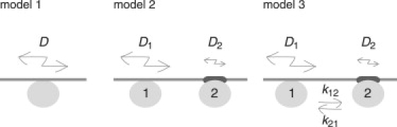
Three models describing the diffusion process of molecules on the membranes.

Numerical simulations

The motion of diffusing molecules is described by the Langevin equation given by

$$\frac{dx\left(t\right)}{dt}={\eta }_x\left(t\right),\frac{dy\left(t\right)}{dt}={\eta }_y\left(t\right),$$ (1)

where x(t) and y(t) indicate the position on the membrane, and η_x(t) and η_y(t) are Gaussian white noises satisfying 〈η_i(t)〉 = 0 and 〈η_i(t)η_j(t′)〉 = 2Dδ_{{i, j}}δ (t-t′) with i, j = x or y, and D being the diffusion coefficient of a given molecular state. For numerical simulations, Eq. 1 is solved by the Euler scheme with a time step δt = 0.001. The initial position is set at the origin, (x, y) = (0, 0). In model 2, the state of a molecule is determined randomly to be one of two states with probability p for state 1 and 1-p for state 2. In model 3, the initial state of a molecule is given in the same manner as model 2, but by using k₂₁/(k₁₂ + k₂₁) instead of p, which ensures that the state distribution is in equilibrium. Whether the state transition occurs during the next time interval, δt, from state 1 to 2 or from 2 to 1 is stochastically determined by comparing a uniformly distributed random number and the transition probability, k₁₂δt or k₂₁δt. The data set for each model consists of 100 trajectories, each of which contains 300 time points. We performed a statistical analysis of the simulated trajectories using MATLAB (The MathWorks, Japan) programs, which are available from the authors.

Displacement and correlation function of squared displacement

From the position of a molecule (x (t), y (t)) at time t = mδt, the displacement, Δr, during an arbitrary time interval, Δt = nδt, is given by

$$\Delta r=\sqrt{{\left(x(t+\Delta t)-x\left(t\right)\right)}^2+{\left(y(t+\Delta t)-y\left(t\right)\right)}^2}=\sqrt{{\left(x(m\delta t+n\delta t)-x\left(m\delta t\right)\right)}^2+{\left(y(m\delta t+n\delta t)-y\left(m\delta t\right)\right)}^2},$$

where m is successive time points along one trajectory (m = 0,1,2,…,F), F is the last time point along one trajectory, and n is the number of time intervals during a displacement measurement.

To calculate the time correlation function of squared displacements, we used a time series of squared displacements in the x direction during a time interval between t and t + Δt, with Δt = nδt given by $\Delta x_i^2\left(t\right)={\left(x_i(t+\Delta t)-x_i\left(t\right)\right)}^2={\left(x_i(m\delta t+n\delta t)-x_i\left(m\delta t\right)\right)}^2$ for the i-th molecule. The time correlation function of squared displacements is defined as

$$C\left(\tau \right)=\langle \Delta x^2\left(t\right)\Delta x^2(t+\tau )\rangle ,$$ (2)

where the average is taken over the ensemble and time. The same time correlation can be obtained by using squared displacements in the y direction as long as there is no anisotropy in the diffusion directions.

Results and Discussion

Theory

Model 1: simple diffusion with a single diffusion coefficient

For a molecule that shows simple diffusion with a diffusion coefficient D, the two-dimensional diffusion equation is written as

$$\frac{\partial P(x,y,t)}{\partial t}=D\left(\frac{{\partial }^2}{\partial x^2}+\frac{{\partial }^2}{\partial y^2}\right)P(x,y,t),$$ (3)

where P(x, y, t) represents the PDF at position x, y and time t. By transforming variables x and y into distance r from the origin, the PDF is obtained from Eq. 3 as follows:

$$P(r,t)dt=\frac{r}{2Dt}{e}^{-\frac{r^2}{4Dt}}dr\text{.}$$ (4)

This represents the probability that a molecule will be found at a distance r at time t. The temporal change in the PDF is shown in Fig. 2 A, where the plot becomes broader with the single peak shifted rightward upon time passages.

Figure 2.

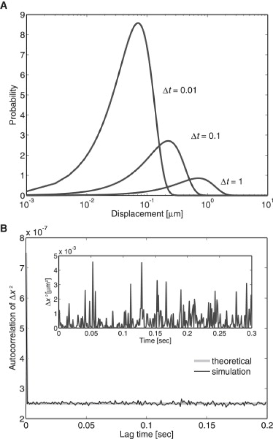
Simple diffusion process with a single diffusion coefficient (model 1). (A) Temporal evolution of the PDF of displacements. Theoretical curves at t = 0.01, 0.1, and 1 are shown for D = 0.25. (B) The autocorrelation function of the squared displacements calculated from 100 trajectories, each containing 300 time points. (Inset) Time series of squared displacements in which a molecule moved in the x-direction with D = 0.25 during the time interval Δt = 0.001. D, μm²/s; t, seconds.

For the purpose of revealing state transitions from the trajectories, we introduced an autocorrelation function of squared displacements per unit time. The Brownian movement of a molecule is driven by thermal molecular collisions that occur at >10¹² times per second in random directions along the membranes. If conditions surrounding the molecule do not change temporally, physical quantities that characterize the mobility of the molecule, such as velocity, exhibit no time correlation under the timescale of observation (at least 10⁻⁵ s). However, in the presence of a state transition, the velocity determined at neighboring time steps, v = (Δx²+Δy²)^1/2/Δt, is correlated (data not shown). For convenience, the autocorrelation function of the squared displacement in the x-coordinate, Δx², can be used instead of v to distinguish whether molecules exhibit simple diffusion or not. The displacement, Δx, is not suitable for examining the state transition, as Δx itself does not cause the temporal correlation. The time series of Δx exhibits both positive and negative values around the average 0, and the autocorrelation function of Δx always vanishes regardless of state transitions. For simple diffusion, the autocorrelation function is a δ correlated as

$$\langle {(\Delta x\left(t\right))}^2{(\Delta x(t\prime ))}^2\rangle =\{\begin{array}{c}4D^2\Delta t^2,t\ne t\prime \\ 12D^2\Delta t^2,t=t\prime \end{array}\text{.}$$ (5)

The time trajectories of the squared displacement in the x direction during a time interval Δt were obtained numerically. The correlation function was then calculated and can be seen to follow the theoretical curve in Fig. 2 B.

Model 2: mixture of two simple diffusion processes

If a mobile molecule has two states but no state transitions, the population of the molecule can be analyzed as a mixture of two simple diffusion processes. Assuming that the proportion of molecules in state 1 is p, the PDF is written by a summation of PDFs for two simple diffusion processes as follows:

$$P(r,t)dt=p\frac{r}{2D_{1}t}{e}^{-\frac{r^2}{4D_{1}t}}dr+(1-p)\frac{r}{2D_{2}t}{e}^{-\frac{r^2}{4D_{2}t}}dr\text{.}$$ (6)

Fig. 3 A illustrates the plots of the PDF at given times. Each plot is composed of two plots derived individually from two simple diffusion processes with diffusion coefficients D₁ and D₂, respectively. The ratio, p, is constant with time, meaning that two independent populations of molecules exist irrespective of time.

Figure 3.

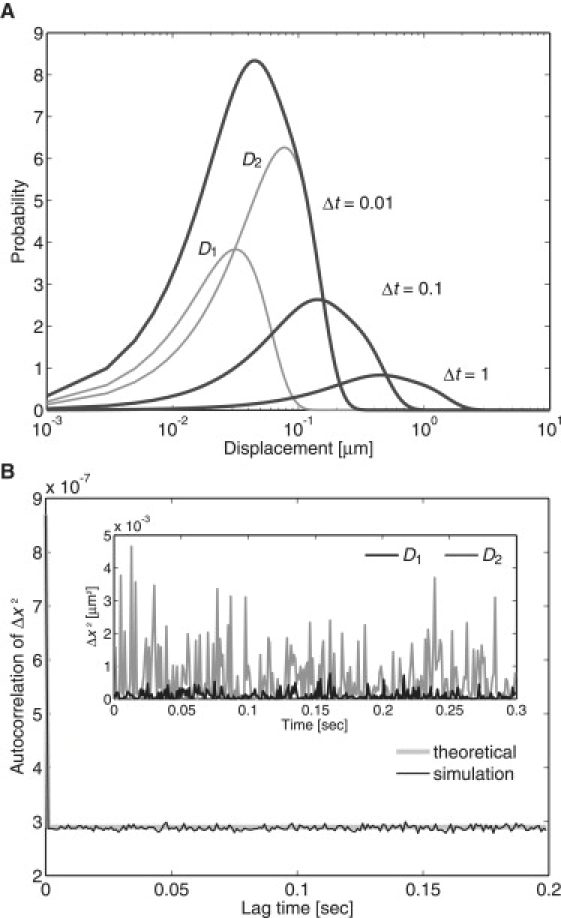
Mixture of two simple diffusion processes (model 2). (A) Temporal evolution of the PDF of the displacements. Theoretical curves at t = 0.01, 0.1, and 1 are shown for D₁ = 0.05, D₂ = 0.3, and p = 0.2 (dark gray lines). Each curve is a superposition of two simple diffusion functions. D₁ and D₂ are shown for t = 0.01 (pale gray lines). (B) The autocorrelation function of the squared displacements calculated from 100 trajectories, each containing 300 time points, in which 20 trajectories were simulated using D₁ = 0.05 and the rest using D₂ = 0.3. (Inset) Time series of squared displacements in which a molecule moved in the x-direction during the time interval Δt = 0.001. The trajectory was made by a numerical simulation assuming a molecule with simple diffusion at D₁ = 0.05 (black line) or D₂ = 0.3 (gray line). D, μm²/s; t, seconds.

Since each molecule exhibits simple diffusion without state transitions, the autocorrelation function of the squared displacement of individual molecules should again behave like a δ-function. By averaging the individual autocorrelation functions over an ensemble, the averaged autocorrelation function is obtained as

$$\langle {(\Delta x\left(t\right))}^2{(\Delta x(t\prime ))}^2\rangle =\{\begin{array}{c}4(p{D}_1^2+(1-p)D_2^2)\Delta t^2,t\ne t\prime \\ 12(p{D}_1^2+(1-p)D_2^2)\Delta t^2,t=t\prime \text{.}\end{array}$$ (7)

The time series of the squared displacements are shown in Fig. 3 B. The amplitude of the fluctuation is dependent on the diffusion coefficient of the individual molecules. In fact, the ensemble average of the autocorrelation function from the simulated trajectories obeys the theoretical curve, which describes molecules are diffusing simply with two different diffusion coefficients (Fig. 3 B).

Model 3: diffusion with state transitions

We also studied diffusive molecules showing transitions between two states with different diffusion coefficients. Since the state transitions affect the PDF of the molecules, the reactions of the state transitions should be taken into account in the diffusion equations. The PDF for a molecule in state 1 or state 2 at position (x, y) at time t is represented by P₁ or P₂, respectively, as follows:

$$\begin{array}{l}\frac{\partial P_1(x,y,t)}{\partial t}=D_1\left(\frac{{\partial }^2}{\partial x^2}+\frac{{\partial }^2}{\partial y^2}\right)P_1(x,y,t)-k_{12}{P}_1(x,y,t)+k_{21}{P}_2(x,y,t)\\ \frac{\partial P_2(x,y,t)}{\partial t}=D_2\left(\frac{{\partial }^2}{\partial x^2}+\frac{{\partial }^2}{\partial y^2}\right)P_2(x,y,t)+k_{12}{P}_1(x,y,t)-k_{21}{P}_2(x,y,t)\end{array},$$ (8)

where$\iint \left(P_1(x,y,t)+P_2(x,y,t)\right)dxdy=1$. The PDF in Eq. 8 was solved analytically by taking the Fourier-Bessel transformation. To obtain the PDF, an inverse transformation was performed by numerical integration for simplicity. We noticed that for a sufficiently short time, t, the PDF is approximately the same as that of model 2 for the same diffusion coefficients, D₁ and D₂, and p = k₂₁/k, where k = k₁₂ + k₂₁ (Fig. 4 A). This is because at an ideally short sampling time, the molecule exhibits hardly any state transitions. In other words, a high temporal resolution makes it possible to analyze two diffusion coefficients for molecules as described by model 2. On the other hand, for a sufficiently longer time interval, the PDF approaches the same profile of model 1 with a single effective diffusion coefficient, D_eff = (D₁k₂₁ + D₂k₁₂)/k. When the overall displacement is measured while state transitions occur with sufficient frequency, all molecules effectively exhibit the same diffusion coefficient, D_eff, irrespective of their initial state. D_eff is an average of the two diffusion coefficients under equilibrium conditions, meaning that the low temporal resolution provides only time-averaged behavior and is indistinguishable from model 1.

Figure 4.

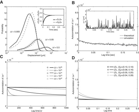
Diffusion process with state transitions (model 3). (A) Temporal evolution of the PDF of the displacements. Theoretical curves at t = 0.005, 0.05, and 0.5 are shown for D₁ = 0.05, D₂ = 0.3, k₁₂ = 20, and k₂₁ = 5. The theoretical curves from model 1 with D = 0.25 (large dotted lines) and model 2 with D₁ = 0.05, D₂ = 0.3, and p = 0.2 (small dotted lines) show a similar profile at t = 0.5 and t = 0.005, respectively. (Inset) Apparent diffusion coefficients of the molecules when state 1 or 2 is adopted at t = 0. (B) The autocorrelation function of squared displacements calculated from 100 trajectories, each containing 300 time points. (Inset) Time series of squared displacements in which a molecule moved in the x-direction during a time interval Δt = 0.001, which was obtained by a numerical simulation using the same parameter values in A. (C) The dependence of the autocorrelation function of the squared displacements on the temporal resolution. By changing the time interval Δt, the theoretical curves using the parameter values from A were plotted against lag time/Δt. (D) The theoretical curves for the autocorrelation function at different D₁ and D₂ ((0.10, 0.10), (0.08, 0.16), (0.05, 0.25), and (0.04, 0.28)) and k₁₂ and k₂₁ values kept constant at 5 and 15, respectively. D, μm²/s; t, seconds, k, 1/s.

The dependence of the apparent diffusion coefficients on the measurement time interval can be explained by considering the transitional behavior of the molecules. Consider two subpopulations of molecules (those in states 1 and 2) at t = 0. The apparent diffusion coefficients averaged over each subpopulation, 〈D₁(t)〉 and 〈D₂(t)〉, are given theoretically as

$$\begin{array}{l}\langle D_1\left(t\right)\rangle =\frac{1}{k}\left\{k_{12}(D_1-D_2)e^{-kt}+D_1{k}_{21}+D_2{k}_{12}\right\},\\ \langle D_2\left(t\right)\rangle =\frac{1}{k}\left\{-k_{21}(D_1-D_2)e^{-kt}+D_1{k}_{21}+D_2{k}_{12}\right\},\end{array}$$ (9)

respectively (see Appendix SB in the Supporting Material for the derivation). At t = 0, 〈D₁(t)〉 and 〈D₂(t)〉 equal D₁ and D₂, respectively, as is expected from the definition of these functions (Fig. 4 A, inset). The apparent diffusion coefficients gradually deviate from D₁ and D₂ with time, which is due to the state transition. As time t increases further, both 〈D₁(t)〉 and 〈D₂(t)〉 approach D_eff. That is, after a transient time interval, the ensemble of each subpopulation reaches its equilibrium state in which the proportion of molecules in states 1 and 2 are k₂₁/k and k₁₂/k, respectively.

The autocorrelation function of displacement distinguishes model 3 from model 2. The autocorrelation function of the squared displacements for model 3 contains an exponential term as given by

$$\langle {(\Delta x\left(t\right))}^2{(\Delta x(t\prime ))}^2\rangle =\{\begin{array}{ll}4\frac{k_{12}{k}_{21}}{k^4}{(D_1-D_2)}^2{e}^{-k(t\prime -t)}(e^{-k\Delta t}+e^{k\Delta t}-2)+4D_{\mathit{eff}}^2\Delta t^2\hfill & t\ne t\prime \hfill \\ 4\frac{k_{12}{k}_{21}}{k^4}{(D_1-D_2)}^2(e^{-k\Delta t}+e^{k\Delta t}-2)+4D_{\mathit{eff}}^2\Delta t^2+8\frac{D_1^2{k}_{21}+D_2^2{k}_{12}}{k}\Delta t^2\hfill & t=t\prime \hfill \end{array}\text{.}$$ (10)

The derivation of the autocorrelation functions is described in Appendix SC in the Supporting Material. Fig. 4 B shows the time series of a displacement that consists of two kinds of durations with different amplitudes in an alternative manner by which the molecule stays in a corresponding state. The time duration of these intervals is distributed exponentially, and the autocorrelation function calculated numerically from the time series shows an exponential decay that is well fit by the theoretical curve (Fig. 4 B). In general, two kinds of intervals with different amplitudes are not necessarily seen in a time series of displacements, even though the molecule follows the kinetic scheme of model 3. Even in such a case, the time correlation for diffusive mobility provides an explicit test to determine whether a molecule shows state transitions during its mobility.

The time resolution of the measurement strongly affects the ability to detect state transitions by autocorrelation analysis (Fig. 4 C). To distinguish model 3 from model 2, the time interval for measurements must be sufficiently longer than the characteristic time of the state transition, whereas to distinguish model 3 from model 1, the temporal resolution must be sufficiently shorter than the characteristic time. When the time interval is shorter than the characteristic time of state transitions, state transitions rarely occur, and thus the molecules behave as if they were described by model 2; therefore, the autocorrelation function may not be distinguishable from a δ-function. On the other hand, when the time interval is much longer than the characteristic time, state transitions will reach equilibrium and the molecules will behave as if they obey the simple diffusion process in model 1. Thus the autocorrelation function is indistinguishable from the δ-function. In addition, higher spatial resolution is needed when the difference between the two diffusion coefficients is small, resulting in a smaller deviation from the δ-function (Fig. 4 D).

Procedure for estimating model type and model parameters

Overview

Here we propose a method to estimate from experimental trajectories both the model type and parameter values such as diffusion coefficients and state transition rates as follows: 1), hypothesize how the molecule behaves on the membrane; 2), construct a diffusion equation appropriate for the hypothetical model; 3), estimate parameter(s) by fitting a distribution of displacements with the PDF derived from the diffusion equation; and 4), confirm the hypothesis by comparing the data with the PDF and estimated parameters. In the main text, we assume that trajectories do not contain noise due to an error in the position measurement. The analysis for the presence of noise is described in Appendix SF in the Supporting Material.

In general, the question of which model type should be applied requires an examination of various factors beyond the three proposed models. Molecules on the membranes of living cells often show dissociation from membranes and/or anomalous diffusion. In addition, the number of states is not necessarily limited to two. Thus, to choose the appropriate model type, the following molecular properties at the membrane should be examined: 1), whether the molecule dissociates from the membranes; 2), whether the molecule exhibits simple diffusion; 3), the number of states that can be distinguished by the diffusion coefficient; and 4), whether the molecule exhibits transitions between states. Dissociation from the membrane can be detected by comparing the fluorescent lifetimes of molecules on the membranes with the photobleaching time of the fluorophore (4,22). Anomalous diffusion can be analyzed by using the MSD, as reported previously (18). To estimate the number of diffusion states, the Akaike information criterion (AIC) can be used as an objective criterion, as discussed below (23). For the detection of state transitions, an autocorrelation function of squared displacements can be used. To further explain the procedure needed to analyze state transitions, below we discuss three cases in which the simulation is performed based on three models. Note that when model 3 is applied, the MSD analysis cannot reliably determine the diffusion coefficients or the state transition rates, even for a relatively simple case (Appendix SA in the Supporting Material). For more-complicated cases that include a combination of multiple states with different diffusive properties, several hypotheses will have to be tested before the most likely model is established, meaning that steps 1–4 must be done repeatedly.

Model 1: simple diffusion process

Stochastic trajectories of molecules moving with simple diffusion were obtained by numerical simulations using D = 2. At first, the number of states with different diffusion coefficients was estimated using the AIC, which serves as an objective index for the probability that the data will follow the hypothetical model. The displacement values during time interval δt were measured and collected from the trajectories to obtain a distribution of displacements (Fig. 5 A). To maximize the ability to detect multiple states, time intervals with a minimum length are ideal because they provide maximum temporal resolution. To examine four hypothetical models in which the molecule has one to four states with different diffusion coefficients, we calculated the AIC values for each model using separate PDFs (see Appendix SD in the Supporting Material for the calculation). The calculation of AIC values requires a maximum likelihood estimation (MLE) of the parameters in each model. The log likelihood, which is a function of the parameter θ, is calculated from data r_n and a hypothesized PDF, P(r|θ), as follows:

$$l\left(\theta \right)=\sum _{i=1}^n\log P\left(r_i|\theta \right),$$ (11)

where θ is estimated from the data set of displacements assuming that the data set is derived from the hypothesized PDF with θ as an unknown parameter vector. The parameter value is sought so that the maximum log likelihood can be returned. Both the diffusion coefficient and the log likelihood were obtained for the four hypothetical models. The AIC values, AIC_i (where the subscript indicates the number of states) were obtained using corresponding log likelihoods. As summarized in Table S1, the minimum AIC value was obtained when a single state was assumed, indicating that the molecule most likely has a single state that can be identified by its diffusion coefficient. For the hypothetical model with a single state, the estimated D-value was 2.011. This coincides well with D = 2, which was used to generate the stochastic trajectories (Fig. 5 A). Consistent with this result, there was no time correlation in the squared displacements (Fig. 5 B). Furthermore, the estimated D-value was consistent for all distributions of displacements during different time intervals (Fig. 5 C). Thus, model 1 is the most appropriate of the three models.

Figure 5.

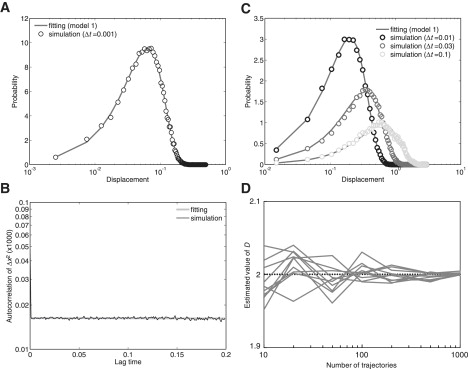
Estimation of the diffusion coefficient for model 1. (A) Histogram of displacements obtained from simulated trajectories. Numerical simulations were performed assuming 100 molecules, each containing 300 time points, showing simple diffusion with D = 2. Molecule displacement during a time interval of 0.001 was calculated. The diffusion coefficient was estimated to be 2.011 according to MLE. The probability density function of model 1 in which the estimated diffusion coefficient was introduced fitted well to the distribution. The x-axis is in log-scale. The data show an abrupt change in slope at the second-smallest data point. (B) The autocorrelation function of the squared displacements calculated from the simulated trajectories. (C) Histograms of displacements where molecules moved during different time intervals of 0.01, 0.03, and 0.1 calculated from the simulated trajectories. The theoretical curves coincide with the histograms. (D) The variance of the estimated diffusion coefficients. The variance decreased inversely with the size of the data set. D, μm²/s; t, seconds.

The estimated values contained some variance due to stochastic fluctuations in the data. In Fig. 5 D, the estimated D-values are shown for data sets containing different numbers of trajectories. Although the mean values of the estimation are approximately equal to the true value irrespective of the number of trajectories, the variance becomes larger when the number of trajectories becomes smaller. This numerical simulation suggests that at least 100 trajectories, each with 300 time points, provide good estimates for the diffusion coefficient. A duration of 300 time points at video rate (33 ms intervals) corresponds to 10 s, which is approximately the same as the photobleaching time of tetramethylrhodamine. When the fluorophores attached to membrane-integrated molecules are visualized using total internal reflection fluorescence microscopy, 1/e (i.e., 37%) are still detectable after 10 s. Therefore, to obtain trajectories of 100 molecules for 10 s, at least 270 molecules should be initially detected.

Model 2: mixture of two simple diffusion processes

Two examples of numerical simulations—one fairly straightforward, the other more complex—were performed: D₁ = 1, D₂ = 5, and p = 0.75 (case 1) and D₁ = 1, D₂ = 2, and p = 0.1 (case 2). Here the procedure described refers to case 1. Details for case 2 are shown in Appendix SE in the Supporting Material.

In case 1, the number of states with different D-values was predicted as 2 by the AIC analysis (Table S2). Accordingly, the estimation using the PDF from Eq. 6 explained well the distribution of displacements (Fig. 6 A). To examine whether the molecules exhibited a transition between the two states, the autocorrelation of squared displacements was analyzed. The result followed the δ-function (Fig. 6 B), indicating that the molecules in case 1 have two states with different D-values and exhibit no transition between them (model 2). The estimated values for D₁, D₂, and p were 1.003, 5.122, and 0.722 (Table S2), respectively, which explains all of the distributions of displacements examined at different time intervals (Fig. 6 C). Therefore, it was concluded that the behavior of the molecules could be successfully explained by model 2. The precision in parameter estimation was inversely proportional to the size of the data set (Fig. 6 D).

Figure 6.

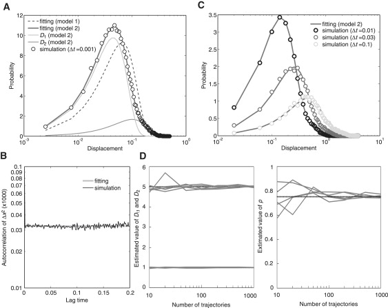
Estimation of parameters for model 2. (A) Histograms of displacements during a time interval of 0.001 obtained from numerical simulations assuming 100 molecules, each containing 300 time points, using D₁ = 1, D₂ = 5, and p = 0.75. The histograms of displacements were fitted with the probability density function from Eq. 6. The parameters estimated were D₁ = 1.003, D₂ = 5.122, and p = 0.722. (B) The autocorrelation calculated from the simulated trajectories. The plots followed the δ-function, indicating no state transitions. (C) Histograms of displacements where molecules moved during different time intervals of 0.01, 0.03, and 0.1 calculated from the simulated trajectories. The theoretical curves coincide with the histograms from the experimental results. (D) The dependence of the variance of the estimated parameter values on the number of molecules contained in a single data set. D₁, D₂, and p were estimated from five simulation runs and plotted against the number of molecules included in the simulated data. D, μm²/s; t, seconds.

Model 3: diffusion with state transitions

Trajectories generated by numerical simulations based on model 3 using D₁ = 1, D₂ = 5, k₁₂ = 5, and k₂₁ = 15 were analyzed. At first, we estimated the number of states for different D-values by calculating the AIC_i for a histogram of displacements obtained from the trajectories and the corresponding PDFs from the i states. AIC₂ was the minimum AIC value, and the histogram of displacements was better fitted with the PDF for two different diffusion states (Eq. 6) (Fig. 7 A and Table S3). Next, analysis of the autocorrelation of squared displacements showed an exponential decay, indicating a state transition during mobility (Fig. 7 B). Thus, we concluded that model 3 is appropriate and that Eq. 8 should be used as the PDF to estimate parameters such as D and state transition rates from the displacement data. We obtained an estimated value of k = 25.530 from the autocorrelation curve by fitting it to Eq. 10 with a least-squares method, which we then used to constrain k₁₂ and k₂₁. With these constraints, we estimated the diffusion coefficient and transition rates from the data set of displacements using the PDF from Eq. 8, finding D₁ = 1.008, D₂ = 4.952, k₁₂ = 6.183, and k₂₁ = 19.347 by MLE. Because the PDF from Eq. 8 with these parameter values coincided consistently with the histograms of displacements at time intervals ranging from 0.001 to 0.1, the above estimations were confirmed to be reasonable (Fig. 7, A and C).

Figure 7.

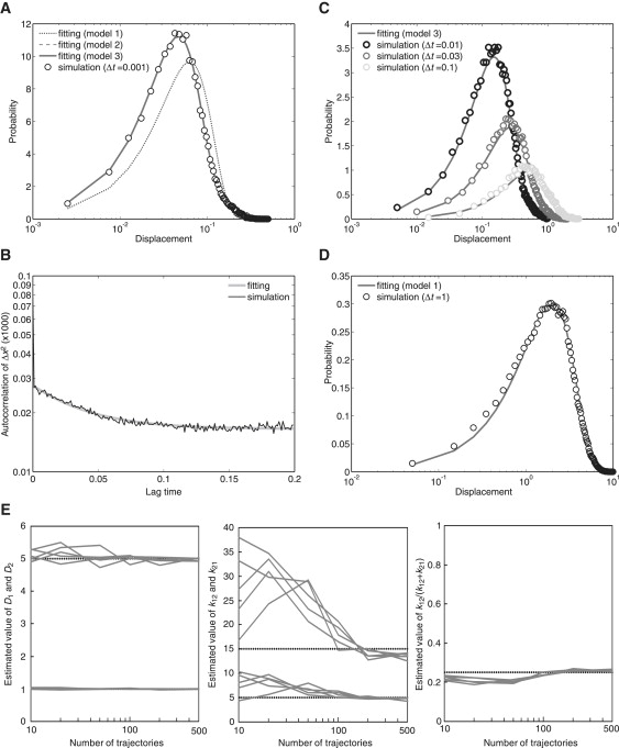
Estimation of parameters for model 3. (A) Histogram of displacements obtained by numerical simulations in model 3 assuming 100 molecules, each containing 300 time points, using D₁ = 1, D₂ = 5, k₁₂ = 5, and k₂₁ = 15. The histogram of displacements during a time interval of 0.001 was better fit using the probability density function from Eqs. 6 and 8 compared to that from Eq. 4, indicating that the molecule has two states with different diffusion coefficients. The parameters estimated were D₁ = 1.008, D₂ = 4.952, k₁₂ = 6.183, and k₂₁ = 19.347. (B) The autocorrelation calculated from the simulated trajectories. The plot shows an exponential decay, indicating that the molecule undergoes state transitions. (C) Histograms of displacements in which molecules moved during different time intervals of 0.01, 0.03, and 0.1, calculated from the simulated trajectories. The theoretical curves coincide with the histograms from the experimental results. (D) Histogram of displacements during a time interval of 1 obtained from 1000 trajectories, each containing 1500 time points. Model 1 could also explain the results obtained when using D = 1.998. (E) Dependence of the variance of the estimated values on the number of molecules contained in a single data set. The values D₁, D₂, k₁₂, k₂₁, and k₁₂/k were estimated from five simulation runs and plotted against the number of molecules included in the simulated data. D, μm²/s; t, seconds; k, 1/s.

The precision of the estimated parameters shows a dependence on the number of molecules included in the data set (Fig. 7 E). In particular, the fitting procedure for the autocorrelation function is sensitive to the number of samples, more so than that for the diffusion coefficients or the transition rates. Even if the k-value shows a large deviation from its true value, the two diffusion coefficients and the ratio of k₁₂ to k are estimated fairly precisely. Thus, to obtain precise estimations for model 3, more molecules need to be analyzed as compared with models 1 and 2. In the case of model 3, ∼500 molecules with 300 time points or more are recommended.

The simulated trajectories display the characteristic dependence of the distributions on the time interval of the displacement measurements. In a relatively short time interval, the distribution was explained by model 2, as shown by AIC₂ (Fig. 7 A). On the other hand, a distribution with a relatively long time interval displayed the same profile as the PDF from model 1 (Fig. 7 D). From the data of the shorter time interval, D₁, D₂, and p were estimated to be 1.015, 4.982, and 0.760, respectively, by MLE using Eq. 6, whereas from the data of the longer time interval, D was estimated to be 1.998 using Eq. 4.

In conclusion, this method provides an efficient way to estimate both a model and important dynamic parameters such as diffusion coefficients, the composition of molecules with different states, and transition rates between the states, principally using the distribution of displacements. This method can be easily applied to molecules moving with simple diffusion in more than two states without state transitions. However, when state transitions do occur, it is necessary to construct an appropriate diffusion equation that describes the estimated molecular behavior. Additionally, further studies are needed to analyze the diffusion process during dissociation from the membranes and/or anomalous diffusion from the displacement distribution. To apply the proposed method to these diffusion processes, the diffusion equations will require a modification to include the dissociating reactions or the effect of directed flow or confinements. Further study is also needed to incorporate a method to determine which state the molecule adopts along its trajectory. With this information, the transition kinetics for diffusive mobility states can be revealed in relation to the surrounding microenvironment due to the heterogeneity within the membranes of living cells.

Supporting Material

Appendices with equations, references, tables, and figures are available at http://www.biophysj.org/biophysj/supplemental/S0006-3495(09)01106-0.

References

- 1.Saffman P.G., Delbrück M. Brownian motion in biological membranes. Proc. Natl. Acad. Sci. USA. 1975;72:3111–3113. doi: 10.1073/pnas.72.8.3111. [DOI] [PMC free article] [PubMed] [Google Scholar]
- 2.Gambin Y., Lopez-Esparza R., Reffay M., Sierecki E., Gov N.S. Lateral mobility of proteins in liquid membranes revisited. Proc. Natl. Acad. Sci. USA. 2006;103:2098–2102. doi: 10.1073/pnas.0511026103. [DOI] [PMC free article] [PubMed] [Google Scholar]
- 3.Shibata S.C., Hibino K., Mashimo T., Yanagida T., Sako Y. Formation of signal transduction complexes during immobile phase of NGFR movements. Biochem. Biophys. Res. Commun. 2006;342:316–322. doi: 10.1016/j.bbrc.2006.01.126. [DOI] [PubMed] [Google Scholar]
- 4.Matsuoka S., Iijima M., Watanabe T.M., Kuwayama H., Yanagida T. Single-molecule analysis of chemoattractant-stimulated membrane recruitment of a PH-domain-containing protein. J. Cell Sci. 2006;119:1071–1079. doi: 10.1242/jcs.02824. [DOI] [PubMed] [Google Scholar]
- 5.Tani T., Miyamoto Y., Fujimori K.E., Taguchi T., Yanagida T. Trafficking of a ligand-receptor complex on the growth cones as an essential step for the uptake of nerve growth factor at the distal end of the axon: a single-molecule analysis. J. Neurosci. 2005;25:2181–2191. doi: 10.1523/JNEUROSCI.4570-04.2005. [DOI] [PMC free article] [PubMed] [Google Scholar]
- 6.Bannai H., Lévi S., Schweizer C., Dahan M., Triller A. Imaging the lateral diffusion of membrane molecules with quantum dots. Nat. Protocols. 2006;1:2628–2634. doi: 10.1038/nprot.2006.429. [DOI] [PubMed] [Google Scholar]
- 7.Ehrensperger M.V., Hanus C., Vannier C., Triller A., Dahan M. Multiple association states between glycine receptors and gephyrin identified by SPT analysis. Biophys. J. 2007;92:3706–3718. doi: 10.1529/biophysj.106.095596. [DOI] [PMC free article] [PubMed] [Google Scholar]
- 8.van Haastert P.J., Postma M. Biased random walk by stochastic fluctuations of chemoattractant-receptor interactions at the lower limit of detection. Biophys. J. 2007;93:1787–1796. doi: 10.1529/biophysj.107.104356. [DOI] [PMC free article] [PubMed] [Google Scholar]
- 9.Turing A.M. The chemical basis of morphogenesis. Phil. Trans. R. Soc. B. 1952;237:37–72. [Google Scholar]
- 10.Chen Y., Lagerholm B.C., Yang B., Jacobson K. Methods to measure the lateral diffusion of membrane lipids and proteins. Methods. 2006;39:147–153. doi: 10.1016/j.ymeth.2006.05.008. [DOI] [PubMed] [Google Scholar]
- 11.Marguet D., Lenne P.F., Rigneault H., He H.T. Dynamics in the plasma membrane: how to combine fluidity and order. EMBO J. 2006;25:3446–3457. doi: 10.1038/sj.emboj.7601204. [DOI] [PMC free article] [PubMed] [Google Scholar]
- 12.Edidin M., Zagyansky Y., Lardner T.J. Measurement of membrane protein lateral diffusion in single cells. Science. 1976;191:466–468. doi: 10.1126/science.1246629. [DOI] [PubMed] [Google Scholar]
- 13.Axelrod D., Koppel D.E., Schlessinger J., Elson E., Webb W.W. Mobility measurement by analysis of fluorescence photobleaching recovery kinetics. Biophys. J. 1976;16:1055–1069. doi: 10.1016/S0006-3495(76)85755-4. [DOI] [PMC free article] [PubMed] [Google Scholar]
- 14.Magde D., Elson E., Webb W.W. Thermodynamic fluctuations in a reacting system-measurement by fluorescence correlation spectroscopy. Phys. Rev. Lett. 1972;29:705–708. [Google Scholar]
- 15.Selvin P.R., Ha T. Cold Spring Harbor Laboratory Press; New York: 2008. Single-Molecule Techniques: A Laboratory Manual. [Google Scholar]
- 16.Qian H., Sheetz M.P., Elson E.L. Single particle tracking. Analysis of diffusion and flow in two-dimensional systems. Biophys. J. 1991;60:910–921. doi: 10.1016/S0006-3495(91)82125-7. [DOI] [PMC free article] [PubMed] [Google Scholar]
- 17.Saxton M.J. Single-particle tracking: the distribution of diffusion coefficients. Biophys. J. 1997;72:1744–1753. doi: 10.1016/S0006-3495(97)78820-9. [DOI] [PMC free article] [PubMed] [Google Scholar]
- 18.Kusumi A., Sako Y., Yamamoto M. Confined lateral diffusion of membrane receptors as studied by single particle tracking (nanovid microscopy). Effects of calcium-induced differentiation in cultured epithelial cells. Biophys. J. 1993;65:2021–2040. doi: 10.1016/S0006-3495(93)81253-0. [DOI] [PMC free article] [PubMed] [Google Scholar]
- 19.Saxton M.J., Jacobson K. Single-particle tracking: applications to membrane dynamics. Annu. Rev. Biophys. Biomol. Struct. 1997;26:373–399. doi: 10.1146/annurev.biophys.26.1.373. [DOI] [PubMed] [Google Scholar]
- 20.Fujiwara T., Ritchie K., Murakoshi H., Jacobson K., Kusumi A. Phospholipids undergo hop diffusion in compartmentalized cell membrane. J. Cell Biol. 2002;157:1071–1081. doi: 10.1083/jcb.200202050. [DOI] [PMC free article] [PubMed] [Google Scholar]
- 21.Kusumi A., Nakada C., Ritchie K., Murase K., Suzuki K. Paradigm shift of the plasma membrane concept from the two-dimensional continuum fluid to the partitioned fluid: high-speed single-molecule tracking of membrane molecules. Annu. Rev. Biophys. Biomol. Struct. 2005;34:351–378. doi: 10.1146/annurev.biophys.34.040204.144637. [DOI] [PubMed] [Google Scholar]
- 22.Hibino K., Watanabe T.M., Kozuka J., Iwane A.H., Okada T. Single- and multiple-molecule dynamics of the signaling from H-Ras to cRaf-1 visualized on the plasma membrane of living cells. Chem. Phys. Chem. 2003;14:748–753. doi: 10.1002/cphc.200300731. [DOI] [PubMed] [Google Scholar]
- 23.Akaike H. A new look at the statistical model identification. IEEE Trans. Automat. Contr. 1974;19:716–723. [Google Scholar]
Associated Data
This section collects any data citations, data availability statements, or supplementary materials included in this article.