MATLAB Toolbox for Functional Connectivity

Abstract

The term “functional connectivity” is used to denote correlations in activation among spatially-distinct brain regions, either in a resting state or when processing external stimuli. Functional connectivity has been extensively evaluated with several functional neuroimaging methods, particularly PET and fMRI. Yet these relationships have been quantified using very different measures and the extent to which they index the same constructs is unclear. We have implemented a variety of these functional connectivity measures in a new freely-available MATLAB toolbox. These measures are categorized into two groups: whole time-series and trial-based approaches. We evaluate these measures via simulations with different patterns of functional connectivity and provide recommendations for their use. We also apply these measures to a previously published fMRI data set (Siegle et al. 2003; 2007) in which activity in dorsal anterior cingulate cortex (dACC) and dorsolateral prefrontal cortex (DLPFC) was evaluated in 32 control subjects during a digit sorting task. Though all implemented measures demonstrate functional connectivity between dACC and DLPFC activity during event-related tasks, different participants appeared to display qualitatively different relationships.

Introduction

The brain forms a distributed network, whereby specialized regions communicate with each other to process information [Cohen and Tong, 2001, Toga and Mazziotta, 2002]. The attempt to identify and quantify such inter-regional relationships has been termed “connectivity” analysis [Friston, 1994]. Functional connectivity (FC), in particular, is defined as the statistical association or dependency among two or more anatomically distinct time-series [Friston et al., 1996, Horwitz, 2003, Salvador et al., 2005]. Measures of FC are agnostic regarding causality or direction of connections.

FC analyses were first performed on human brain functional data using positron emission tomography (PET) [Clark et al., 1984, Horwitz et al., 1984, Friston et al., 1993], and have since expanded into functional Magnetic Resonance Imaging (fMRI), Magnetoencephalography (MEG), Electroencephalography (EEG), and peripheral physiological measures [Friston, 1994, Sun et al., 2004, Salvador et al., 2005, David et al., 2004, Chen et al., 2008, Jeong et al., 2001, Na et al., 2002, Gianaros et al., 2005]. FC has also been assessed with a variety of different experimental designs, including block designs [Hampson et al., 2002, Koshino et al., 2005, Anand et al., 2005a] and event-related designs [Rissman et al., 2004, Fox et al., 2006, Siegle et al., 2007, Aizenstein et al., 2009]. Block designs alternate periods of stimulus types, with each period presenting a given stimulus type multiple times, whereas event-related designs present stimuli individually separated by an interstimulus interval (ISI), termed a “trial”. More recently, resting state studies, particularly involving the “default mode” network [Biswal et al., 1995, Lowe et al., 1998, Greicius et al., 2008, Fransson, 2005], have also become popular for determining connectivity. Methods for computing FC from resting state data usually assume that the time-series are stationary (i.e., probabilistically unchanging across time), and utilize information from the entire time-series of fMRI scans (“whole time-series” approaches). Conversely, methods for event-related designs do not require stationarity, and FC is often computed based on associations obtained by examining data divided into individual trials (“trial-based” approaches). Block designs may be considered locally stationary and hence are intermediate between resting state and event-related designs.

The MATLAB toolbox described in this paper includes measures of FC from both whole time-series and trial-based approaches, including zero-order and cross-correlation [Biswal et al., 1995, Anand et al., 2005b, Siegle et al., 2007], cross-coherence [Sun et al., 2004, Salvador et al., 2005, Murias et al., 2007], mutual information [Jeong et al., 2001, Na et al., 2002, Salvador et al., 2005], peak correlation [Rissman et al., 2004], and functional canonical correlation [Worsley et al., 2005, Siegle et al., 2007]. We also implement optional temporal smoothing steps in the toolbox. Many of these measures have not been previously available in a user-friendly package aimed at neuroscientists and this toolbox provides quick and easy means to compute and compare results from different FC measures. A classication analysis via a tree-building algorithm [Breiman, 1993] is conducted using the values of multiple FC measures to predict the pattern of connectivity relationships between regions.

The implemented techniques specifically attempt to characterize the relationships between time-series extracted from two or more regions above and beyond zero-order correlational relationships, potentially controlling for one or more other time-series. The toolbox does not include other types of measures of FC. Following Cattel (1952), data can be clustered along dimensions of occasions (time), variables (for fMRI, space or region), and person. We have concentrated on characterizing relationships between occasions across regions; e.g., lagged cross-correlation analysis characterizes relationships of a time-series at one lag to another time-series at other lags. FC has been alternately defined in the literature based on other ways of clustering fMRI data. For example, techniques such as principal components analysis (PCA) or independent components analysis (ICA) generally attempt to cluster voxels or regions (i.e., variables). ICA, in particular, extracts latent time-series which characterize the behavior of sets of voxels (e.g., Formisano et al. 2004). The degenerate case of spatial PCA with just two regions is the zero-order correlation between the regions. Thus, these techniques are more appropriate when large numbers of voxels or regions are examined. Other techniques such as the examination of psychophysiological interactions (Friston et al. [1997]) do not control for third-variable time-series, but rather, examine interactions with them. Such alternate techniques generally focus on zero-order relationships between time-series, but could be generalized to account for the types of relationships examined in this paper.

Materials and Methods

I. Overview of How to Use the Toolbox

The Functional Connectivity Toolbox is developed in MATLAB (Mathworks, Inc.) as an open source package. It is designed to use existing routines in the MATLAB distribution with an additional freely-available toolbox for functional data analysis (Ramsay 2005; http://www.psych.mcgill.ca/misc/fda/index.html). Each FC measure listed above is coded into a function in MATLAB. The inputs of the functions are equal length time-series data from brain regions’ responses within a single subject. For slow event-related designs, the user must also indicate the number of scans per trial. For example, if Y₁(t) and Y₂(t) are one subject’s fMRI responses from two brain regions for an slow event-related design with T scans per trial, then the peak correlation between Y₁ and Y₂ can be obtained by entering corrpeak(Y₁, Y₂, T), where corrpeak is the function’s name, as defined in MATLAB. For fast event-related designs, stimulus time-series should be indicated instead of scans per trial. Calling features for each of the functions in the toolbox, along with its arguments are described in the Appendix.

II. Smoothing

We also include an optimized smoothing step as a noise-reduction procedure because not all noise can be removed or cleaned [Lazar, 2008]. Temporal smoothing is particularly important in connectivity analyses because reliable detection of FC between brain responses can require high signal-to-noise ratio (SNR) [Astolfi et al., 2005]. FC estimates are therefore strongly dependent on the level of temporal smoothing; too much smoothing yields over-estimates of relationships between time-series whereas too little smoothing underestimates these relationships. We have implemented an optional Bayesian temporal smoothing technique using a Markov Chain Monte Carlo (MCMC) Gibbs sampling algorithm with roughness penalty parameters treated as components of variance and estimated from the data. This technique utilizes a cubic B-spline basis expansion with equally spaced knots, and includes the ability to handle white or autoregressive lag-1 structured (AR(1)) noise. An optional pre-whitening step is also available with AR(1) noise. The level of autocorrelation has to be predetermined; the default value is set to 0.7. We chose a cubic B-spline basis because it produces smooth yet flexible fits and for efficient computation of the roughness penalty parameter. A simple default choice of the number of knots for the basis is $\mathit{min}(\frac{1}{4}\times \text{length}\text{of}\text{data},35)$ [Ruppert et al., 2003].

III. Whole Time-Series Approaches

Whole time-series approaches aim to examine the relationships contained within the entire time-series of fMRI scans, based on the assumption that the time-series is stationary. Stationarity of the time-series guarantees that the relationships among them are probabilistically consistent over time [Shumway and Stoffer, 2006].

Cross-Correlation

Zero-order correlation measures the simultaneous linear coupling relationship between two time-series. When the time courses are highly positively correlated, this implies that the two regions are on average more or less active at the same times. Conversely, a high negative correlation implies that when one region is more active the other is less active. Zero-order correlation has been used often to measure inter-regional relationships in fMRI, e.g., in Biswal et al. (1995).

Lagged cross-correlation can also be used to evaluate inter-regional relationships [Siegle et al., 2007]. Lagged cross-correlations capture the lagged or delayed linear relationships between regions. Cross-correlation between brain regions A and B at positive lags indicate a relationship between activity of region A and subsequent activity of region B, or vice versa. One study that used lagged cross-correlations [Siegle et al., 2007] found that depressed people had attenuated correlation of dorsolateral prefrontal cortex activity with amygdala activity 3 to 6 sec later.

Cross-correlation of any two individual time-series (i, j), at lag h, ρ_ij(h), is given by

$${\rho }_{ij}(h)=\frac{co{v}_{ij}(t,t+h)}{\sqrt{va{r}_i(t)va{r}_j(t+h)}},$$ (1)

where ρ_ij(h) = ρ_ji(−h), and is restricted to the [−1, 1] interval. h = 0 corresponds to zero-order correlation.

Correlations are often subtended by low-frequency (less than 0.1 Hz) components of the data, as has been shown in several studies [Biswal et al., 1995, Lowe et al., 1998, Cordes et al., 2001]. Biswal et al. (1995), for example, reported that low-frequency (below 0.08 Hz) correlations existed between the bilateral primary motor cortices (M1) and the supplementary motor area (SMA) during resting state scans. We include the ability to apply a low-frequency filter as an option parameter to the cross-correlation routine. By default this filter is set to 0.1 Hz.

Cross-Coherence

While correlation is defined in the time domain, coherence measures are in the frequency domain. Coherence has been repeatedly shown to be a useful statistic for investigating FC across brain regions [Leopold et al., 2003, Sun et al., 2004, Salvador et al., 2005]. Coherence measures implicitly account for lags in the effects of one region on another. If a time-series in one region is broadly similar to that in another, but with a time delay, then the ordinary zero-order correlation between the two will be moderate or low; the coherence, by contrast, will be high within the bandwidth of the curve. The squared coefficient of coherence can be interpreted as the proportion of the power in one of the two time series (at a selected frequency), which can be explained by its linear regression to the other time course.

The concept of coherence of time-series was introduced by Wiener (1949) and extensively developed and described by Rosenberg et al. (1989) for its applicability to functional imaging data. Spectral coherence for determination of FC was applied to motor experiments by Sun et al. (2004).

Coherence Coh_ij(λ) between any two individual time-series (i, j) at frequency λ is defined as

$$Co{h}_{ij}(\lambda )=\mid R_{ij}(\lambda ){\mid }^2=\frac{\mid f_{ij}(\lambda ){\mid }^2}{f_{ii}(\lambda )f_{jj}(\lambda )},$$ (2)

where R_ij(λ) is the complex valued coherency of Y_i and Y_j; f_ij(λ) is the cross-spectral density between Y_i and Y_j; and f_ii(λ) and f_jj(λ) are the spectral densities of Y_i and Y_j. Coherence is a positive function, it is symmetric in i and j(e.g., Coh_ij(λ) = Coh_ji(−λ)), and bounded by 0 and 1.

Mutual Information

Theoretically, correlation and coherence measure the linear dependence between two time-series, whereas mutual information is a statistical measure of both linear and nonlinear dependence [Shannon and Weaver, 1948]. Mutual information quantifies the shared information between two time-series. For example, if the two time-series are independent, there is no shared information and hence the mutual information is zero. At the other extreme, if one time-series is a deterministic one-to-one function of the other, then they share the same information: in this case their mutual information is infinite.

Jeong et al. (2001) used an entropy-based measure of mutual information to investigate FC among time-series from different cortical areas in both Alzheimer’s disease patients and healthy controls. Salvador et al. (2005) employed mutual information based on coherence and showed that FC lay mainly in low frequencies. Chen et al. (2008) developed a conjoined time-frequency analytical-based method of mutual information to explore brain neural connectivity by MEG during a self-paced finger lifting task. In this toolbox, we implement mutual information based on coherence in the frequency domain [Salvador et al., 2005], which is defined as

$${\delta }_{ij}=-\frac{1}{2\pi }{\int }_{{\lambda }_1}^{{\lambda }_2}\mathit{log}(1-{\mathit{Coh}}_{ij}(\lambda ))d\lambda ,$$ (3)

where [λ1, λ2] specify the frequency band within which to integrate the infomation and −π ≤ λ1 < λ 2 ≤ π. This formula assumes time-series are Gaussian.

This integral is unbounded, ranging from 0 to infinity. A simple transformation can be applied, however, to obtain a normalized mutual information [Joe, 1989, Granger and Lin, 1994, Salvador et al., 2005], with scores in the interval [0, 1]. This is implemented in the toolbox as

$${\phi }_{ij}={[1-\mathit{exp}(-2{\delta }_{ij})]}^{\frac{1}{2}}.$$ (4)

Partial Cross-Correlation/Coherence/Mutual Information

With analyses including more than two brain regions, one question is whether an observed dependence between any two regional time-series is attributable to a direct connection between the two brain regions or to an indirect relationship involving other regions. This question may be addressed by measuring the association between the two regions (i, j) after accounting for the relationship of each to other reference time-series 1, …, P\i, j (time-series from region 1 to P except time-series from region i and j). This is called conditional dependence. A discussion of how to apply bivariate cross-correlation/coherence/mutual information analysis to multivariate time-series was provided by Salvador et al. (2005). Our toolbox includes similar routines for computing partial cross-correlation/coherence/mutual information. These measures yield the partial relationship of each pair of time-series accounting for the remaining time-series in a matrix.

IV. Trial-Based Approaches

Trial-based approaches evaluate trial-to-trial relationships and are usually applied to event-related experimental designs. Time-series of brain regions in trial-based approaches does not have to meet the assumption of stationarity.

Peak Correlation

Peak correlation captures the coupling relationship of peaks in activitation in pairs of brain regions associated with discrete events (trials). We implement this by first creating functional versions of trial-related time-series by temporally smoothing the trial time courses: each trial yields one curve per region. Separate peak estimates are computed from the functional responses for each individual trial and for each region and consequently used as the data in a correlation analysis. A high positive value of peak correlation between two regions indicates that two regions are more or less active than average during the same trials. Similarly, a high negative value implies that when one region has a higher-than-average peak, the other region has a lower-than-average peak.

Functional Canonical Correlation

Functional canonical correlation seeks to investigate which modes of variation between pairs of observed random curves are most associated with one another. Functional versions of trial-related time-series are created by smoothing the trials and the canonical correlation between these functional responses is computed. The functional canonical correlation [Ramsay and Silverman, 1997] between any pair of individual time-series (i, j) is given by

$${\mathit{ccorsq}}_{ij}(\xi ,\eta )=\frac{\mathit{cov}{(\int \xi (t)Y_{im}(t)dt,\int \eta (t)Y_{jm}(t)dt)}^2}{(\mathit{var}\int \xi (t)Y_{im}(t)dt+\lambda \mid \mid D^2(\mathit{\xi })\mid {\mid }^2)(\mathit{var}\int \eta (t)Y_{jm}(t)dt+\lambda \mid \mid D^2(\mathit{\eta })\mid {\mid }^2)}.$$ (5)

Here, ξ(t) is the weight function for Y_i and Y_im refers to the mth trial of region i; similarly, η(t) is the weight function for Y_j and Y_jm refers to mth trial of region j. λ is a smoothing parameter, chosen via cross-validation, that describes the smoothness constraint on the weight functions. ||D²(ξ)||² and ||D²(η)||² represent the roughness of the weight functions, where D²(·) is the second derivative operator.

Qualitative relationships between the two regions can be explored by examining the weight functions. For example, weight functions may indicate that sustained activity on one region is related to peak activity in another region. Siegle et al. (2007) used functional canonical correlation analysis to measure FC between amygdala and DLPFC responses to negative words.

Use of Whole Time-Series Approaches with Nonstationary Designs

The extent to which whole time-series approaches are applicable to nonstationary (e.g., trial-based) designs is unclear. The whole time-series approaches generally assume stationarity, and thus in the case of a recurring effect of a stimulus on two regions, may overestimate true connectivity. This over-estimation might be attenuated by examining connectivity at frequency bands outside the trial range (e.g., using a low-pass filter). Alternately, if effects of the stimulus are assumed to be constant across trials, residual relationships between regions might be inferred to reflect connectivity. In this case, stimulus effects can be explicitly accounted for before computing connectivity, e.g., via residual regressions or partial correlation analysis, entering a stimulus-related response as a covariate. With a fast event-related or jittered design with catch trials, the covariate waveform could be constructed by deriving an impulse response function (e.g., via deconvolution) which could be convolved with the design. In the case of a fast event-related design in which catch trials are not presented, it would be possible to covary a series of canonical responses convolved with the design from the waveforms in both regions. With slow event-related designs, if responses within a region are assumed to have a canonical shape, the covariate waveform could be constructed by convolving a canonical response with a delta function at the stimulus frequency. But systematic deviations from the canonical waveform in either structure might then create a spurious pattern of connectivity. Rather, using the mean responses in each candidate waveform as covariates minimizes these effects by assuming only that trial-to-trial deviations from the mean response in both regions reflect the effects of connectivity. We have adopted this last approach in the simulations described below.

Results

Simulation 1

In Simulation 1, we performed two Monte Carlo studies to illustrate how the implemented FC measures detect different patterns of association between two regions. The first study simulated stationary (resting state) fMRI time-series data for use with whole time-series FC measures. Since any stationary time-series can be represented as the random superposition of sines and cosines oscillating at various frequencies [Shumway and Stoffer, 2006], each regional time-series was generated by a linear combination of sine waveforms of different frequencies and phases; the weights for each component were generated from a normal distribution. The regional time-series were then convolved with an hemodynamic response function (double gamma) to produce a temporally smoothed BOLD time-series. Connectivity between regional time-series was achieved by linking the weights of sine waveforms at certain frequencies and phases. Simulated data was generated as single run for each of fifty subjects, consisting of 140 scans (TR=2s). Gaussian white noise was added to each run. Functional SNR (the ratio between the intensity of a signal associated with changes in brain function and the variability in the data due to all sources of noise [Huettel et al., 2004, Shumway and Stoffer, 2006]) was set to approximately 3 here and in the second study. Simulation and FC results for the first study are given in Figure 1.

Figure 1.

The plots from top to bottom on the far left show one subject’s whole-waveform-based simulated time-series (140 scans) of two regions (blue lines and red lines) for 4 different patterns of association. Results of cross-correlation and cross-coherence shown here are the overall mean across 50 subjects. mu_l, mu h represent mean mutual information over low frequency band and high frequency band respectively.

The second study simulated nonstationary (event-related) fMRI brain responses. The BOLD activation curve for each trial was generated by a linear combination of B-spline basis functions. Weights for the B-splines were generated from multivariate normal distributions with predefined mean and variance. An association between two regions was created by correlating the weights of B-spline basis functions. Simulations were generated with 20 trials and 7 scans per trial (TR=2s) for each of fifty subjects with additive white Gaussian noise. Simulation and FC results for the second study are given in Figure 2.

Figure 2.

The plots from top to bottom on the far left show one subject’s trial-based simulated time-series (20×7 scans) of two regions (blue line and red line) for 11 different patterns of association. Results of FC measures shown here are overall mean across 50 subjects. Red dashed lines shown are partial correlation or coherence. pmul, pmuh, p_c and ca_c represents partial mutual information over low frequency band, partial mutual information over high frequency band, peak correlation, and functional canonical correlation respectively. The shown canonical correlation weight functions of each region (blue line and red line) are the overall mean of weight functions across subjects. Cross-correlation, coherence and mutual information are taken after centering the time-series data from the overall median of each run (20 trials).

In the second study, we also considered partial correlation/coherence/mutual information by including reference waveforms to control for co-activation of regions from application of the stimulus. Correlation and coherence measures can be dominated by the stimulus-locked response in event-related designs. When a stimulus is presented, the stimulus-locked neural response may cause an increase in the BOLD signal in both regions simultaneously (co-activation). This is not necessarily due to an intrinsic task-induced functional coupling, but may be due to the response in both regions to the externally-applied stimuli. For example, in the simulations of event-related design data shown in Figure 2, coherence is particularly high at the trial frequency even when there is no inherent connectivity. By including stimulus reference waveforms, partialling methods estimate any remaining relationship between two time-series after taking co-activation into account. For these simululations we chose two stimulus reference waveforms generated by repeating the mean trial-averaged responses across all trials for each region. Partial results are shown in Figure 2 as dashed red lines.

Tables 1 and 2 summarize the computed FC measures for different patterns of association between two regions, based on the simulation results. Statements within brackets are partial results accounting for stimulus waveforms. For simulations of non-design related connectivity, including the mean stimulus waveforms as covariates does not change the value of correlation and coherence (e.g., zero-order (lag 1) relationship unrelated to the design; relationships only among low frequencies (0.05 Hz) unrelated to design). For all types of relationships related to the design, coherence at the trial frequency is attenuated after including stimulus waveforms. In contrast, cross-correlation is still high at lag 0 (or 1) for relationships of design-induced peak amplitude between two regions (e.g., zero-order (lag 1) relationship related to the design; related peak amplitudes but unrelated latencies; and A-1-mode and B-2-modes) because the two regions become more or less active than the average response during the same trials, a relationship remains after accounting for stimulus waveforms reflecting true connectivity. Cross-correlation attenuates a bit for data with related peak amplitudes and latencies but variability in higher moments, because for some trials region 1 may activate before region 2 and for other trials the reverse may happen. The relationship of A-peak amplitude to B-sustained activity is phase-lagged after accounting for the stimulus waveform, since when region 1 has a higher than average peak, region 2 has higher than average sustained later activity. Partial cross-correlation and partial cross-coherence are very low for data generated with unrelated peak amplitudes but related peak latencies and essentially zero for data generated with stimulus co-activation but no FC relationship. Note, however, that canonical correlation weighting functions for data generated with unrelated peak amplitudes but related peak latencies do indicate the nature of the FC relationship. The two weight functions for this relationship (displayed in Figure 2) are identical and put most weight in the beginning and end of the trials, indicating that the primary mode of covariation lies in shifting the timing of the peaks.

Table 1.

Interpreting data based on simulation results (whole waveform)

Zero-order corr.	Lagged corr.	Cross coh.	Mutual info.(L)	Mutual info.(H)	Interpretation
High	Medium or low	High at low freq.	Medium	Low	Zero order relationship
Medium or low	High	High at low freq.	Medium	Low	Lagged (lag 4) relationship
Could be high	Could be high	High at low freq.	Medium	Low	Multiple frequency components with relationships only among low frequencies
Low	Low high	High at high freq.	Low	Medium	Multiple frequency components with relationships only among high frequencies

Table 2.

Interpreting data based on simulation results (trial-based waveform)

Zero-order corr.	Lagged corr.	Cross coh.	Mutual info. (L)	Mutual info. (H)	Peak corr.	Canonical corr.	Interpretation
High (High)	Medium or low (Medium or low)	High at low freq. (High at low freq.)	Medium (Medium)	Low (Low)	Medium	High	Zero-order relationship unrelated to design
Medium or low (Medium or low)	High (High)	High at low freq. (High at low freq.)	Medium (Medium)	Low (Low)	Low	High	Lagged relationship unrelated to design
High (High)	Medium or low (Medium or low)	High at trial freq. (High at low freq.)	Medium (Medium)	Low (Low)	High	High	Zero-order relationship related to design
Medium or low (Medium or low)	High (High)	High at trial freq. (High at low freq.)	Medium (Medium)	Low (Low)	High	High	Lagged relationship related to design
Could be high (Could be high)	Could be high (Could be high)	High at 0.05 Hz High at 0.05 Hz)	Medium (Medium)	Low (Low)	Medium or low	High	Multiple frequency components with relationships only among low frequencies(0.05Hz) unrelated to design
High or medium (Medium)	Medium or low (Low)	High at trial freq. (Low)	Medium (Low) (Low)	Medium or low	High	Medium	Related peak amplitudes and latencies but variability in higher moments (e.g., skew, kurtosis)
Medium (Medium)	Low (Low)	Medium at trial freq. (Low)	Medium (Medium)	Medium or low (Low)	High	High	Related peak amplitudes but unrelated peak latencies
Medium (High or medium)	Medium or low (High at certain lag)	High at trial freq. (High at low freq.)	Medium (Medium)	Low (Low)	High	High	A-1-mode corresponds to B-2-mode and related mode amplitudes and latencies
Medium (Medium or low)	Low (High at certain lag)	High at trial freq. (High at low freq.)	Medium (Medium)	Low (Low)	Low	High	Relationship of A-peak-amplitude to B-sustained activity
Medium (Low)	Low (Low)	High at trial freq. (Low)	Medium (Low)	Low (Low)	Low	High	Unrelated peak amplitudes but related peak latencies
Low (Low)	Low (Low)	High at trial freq. (Low)	Low (Low)	Low (Low)	Low	Low	No connectivity

Tree-Building

Tables 1 and 2 show that the combination of all FC measures did not exhibit the same pattern for any two simulated connectivity relationships between the two regional time-series. Thus, it appears that quantifying more than one FC measure may be useful in understanding the precise nature of connectivity between two fMRI time-series. To explore this idea further, we determined a set of if-then logical (split) conditions permitted accurate predictions of association type between regions (from the 11 patterns listed in Table 2) from a set of FC measure predictors (partial correlation/coherence/mutual information are implemented instead of correlation/coherence/mutual information). We conducted a classification analysis via a tree-building algorithm [Breiman, 1993] using the values of the FC measures to move through the tree (until reaching a terminal node) to predict the category (1–11) shown for that node. This classification tree is shown in Figure 3. The tree was built based on 80% of the simulation data and the pruning parameter was chosen by 10-fold cross-validation [Venables and Ripley, 2003]. The proportion of correctly classified simulations for the other 20% was 92.7%. The inclusion of multiple measures in the tree suggested that multiple FC measures are useful in determining the true nature of a functional relationship between two regions.

Figure 3.

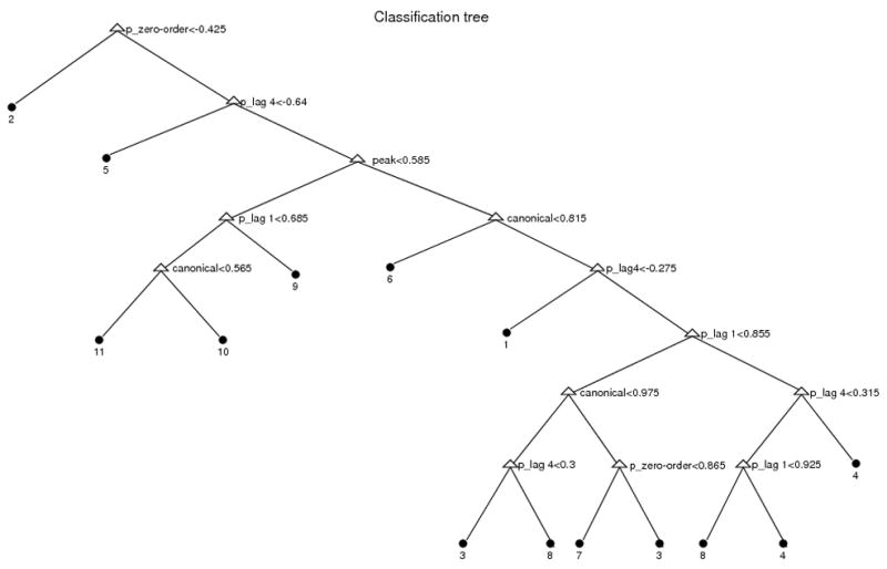
Classification tree of 11 pattern of associations. Here, 1–11 represent: 1. Zero-order relationship unrelated to design; 2. Lagged (lag 4) relationship unrelated to design; 3. Zero-order relationship related to design; 4. Lagged (lag 1) relationship related to design; 5. Relationships among low frequencies unrelated to design; 6. Related peak amplitudes and latencies but variability in higher moments; 7. Related peak amplitudes but unrelated peak latencies; 8. A-1-mode B-2-modes; 9. Relationship of A-peak-amplitude to B-sustained activity; 10. Unrelated peak amplitudes but related peak latencies; and 11. No connectivity. Covariates put in this classification tree were partial zero-order correlation(‘p_zero-order’), partial lag-1 correlation(‘p_lag 1’), partial lag-4 correlation(‘p_lag 4’), partial mutual information over low frequency band(‘pmu_l’), partial mutual information over high frequency band(‘pmu_h’), peak correlation(‘peak’), and functional canonical correlation(‘canonical’).

Simulation 2

In Simulation 2, we performed two Monte Carlo studies to illustrate the effect on computed FC relationships when different types of noise are added to related BOLD signals. BOLD signals were generated as in Simulation 1. In study 1, BOLD signals from two regions were stationary with a zero-order relationship. In study 2, BOLD signals were event-related with zero-order relationship. AR(1) noise with low SNR (functional SNR around 1.5) and AR(1) noise with high SNR (functional SNR around 2.5) were added to the coupled BOLD responses. In each of the studies, FC measures were computed after smoothing with and without explicitly modeling autocorrelated noise. FC results from the two studies are shown in Figure 4 and 5 respectively. These results show that as SNR decreases, FC measures tend to become attenuated. However, even under a high level of noise inter-regional relationsips were detectable for some FC methods; e.g., functional canonical correlation is still high (around 0.8) when applied to smoothed fMRI responses with low SNR (see second row of Figure 5).

Figure 4.

Mean results of different FC measures applied to simulations with zero-order relationship (stationary design) between regions. FC measures were computed after smoothing with and without explicitly modeling autocorrelated noise. Results of data with high SNR are shown in red and results of data with low SNR are shown in blue. 1st row: smoothing without modeling autocorrelated noise; 2nd row: smoothing with modeling autocorrelated noise.

Figure 5.

Mean results of different FC measures applied to simulations with zero-order relationship (event-related design) between regions. FC measures were computed after smoothing with and without explicitly modeling autocorrelated noise. Results of data with high SNR are shown in red and results of data with low SNR are shown in blue. 1st row: smoothing without modeling autocorrelated noise; 2nd row: smoothing with modeling autocorrelated noise.

In addition, the results illustrate that smoothing fMRI responses with a method that explicitly models autocorrelated noise can be important for detecting FC when noise is in fact autocorrelated, especially when the SNR is low. For example, in Figure 5, partial cross-coherence between the two regions is quite small (around 0.2) at low frequencies when the SNR is low and smoothed without modeling autocorrelated noise, but increases to around 0.7 when the data are smoothed with a method that models autocorrelated noise. Smoothing data after pre-whitening (not shown here) resulted in similar improved estimates of FC in the presence of autocorrelated noise. In contrast, we found little difference in the FC measures for the stationary design (Figure 4).

Application to an Empirical Neuroimaging Dataset

This analysis involves data from 32 healthy adult subjects, acquired as part of a larger study. The goal was to determine functional relationships between the dorsal anterior cingulate cortex (dACC) and dorsolateral prefrontal cortex (DLPFC) during executive control. Theoretical models [Cohen and Tong, 2001] and initial neuroimaging analyses [MacDonald et al., 2000, Aizenstein et al., 2009] suggest that bidirectional relationships should be apparent - that is, the DLPFC is involved in executive control necessary to prime the dACC, and dACC activity should spur future DLPFC activity. But these relationships have not been tested using multiple measures of connectivity, so the true nature of relationships has not been determined. In addition, no study of relationships between these regions has considered the idea that different healthy subjects may be characterized by qualitatively different functional relationships among these regions. In 36 slow-event-related trials (one subject with 33), participants viewed a fixation mask (1 sec), followed by a set of three, four or five digits (2 sec), followed by another fixation mask (5 sec). Then, a ‘target’ digit from the previously presented set appeared (10 sec). Participants were told to push a button indicating whether the target was the middle digit of the previously presented set or not. The fMRI data were gathered every 1.5 sec. The full experimental design as well as preprocessing of these data are described by Siegle et al. (2007). Briefly, data were subjected to motion correction, detrending within blocks, and temporal smoothing, cross registered to an image within the dataset, and subjected to spatial smoothing, 6mm FWHM Gaussian kernel. The reference brain was then transformed into Talairach space using AFNI (Cox, 1996) to extract anatomical masks. Regions involved in this analysis were dACC restricted in BA32 and DLPFC restricted in BA9 (Figure 6), with significant scan × condition interactions (p < 0.0001) using a repeated measures Analysis of Variance (ANOVA) in which subject was a random factor and scan and condition (number of presented digits) were fixed factors, subject to an empirically derived contiguity threshold of 105 voxels. Significant regions were restricted to those in BA32 and BA9 using Talairach masks and are shown in Figure 6. The averaged fMRI signal from each ROI(region of interest) were acquired and normalized by subtracting and then divided by the median regional activation across the whole time-series within stimulus types and subjects. Figure 7 shows one subject’s BOLD responses of the ROIs.

Figure 6.

Identified regions of interest used in the analysis: dACC restricted in BA32 (left) and DLPFC restricted in BA9 (right).

Figure 7.

Thirty-six experimental trials for one subject. Blue lines are trials in dACC(BA32) (left panel) and DLPFC(BA9) (right panel). Bold red lines are subject’s mean responses for each ROI.

We applied all of the FC measures (including partial correlation methods, controlling for the mean effect from the external stimulus in each region) to dACC(BA32) and DLPFC(BA9) within subjects. Cross-correlation and partial cross-correlation both reached their maximum at lag 0 and the associations were not attenuated when controlling the effects from the external stimulus. Taking out the external stimulus waveform reduced cross-coherence between these two regions at the trial frequency. A strong relationship was observed for both peak correlation and canonical correlation.

Based on the results of different FC measures on this real dataset, we classified the 32 subjects according to the classification tree shown in Figure 3. There were 6 detected relationships: 3. Zero-order relationship unrelated to design; 6. Related peak amplitudes and latencies but variability in higher moments; 8. A-1-mode B-2-modes; 9. Relationship of A-peak-amplitude to B-sustained activity; 10. Unrelated peak amplitudes but related peak latencies; and 11. No relationship. Most subjects (27 of 32) were classified to relationship 6, 8 and 10 (Figure 8). Average results of the computed FC within three main groups are shown in Figure 9 (partial results are shown in dashed red lines). Subjects classified to relationships 6 and 8 showed higher cross-correlation and peak correlation than subjects classified to relationship 10 because they had related peak amplitude activity between the two regions. Subjects classified to relationship 8 showed higher cross-coherence over low frequency band than the other groups.

Figure 8.

Classification results for 32 subjects. X axis represents the 11 types of association corresponding to Figure 3. Y axis represents the number of subjects classified to each relationship.

Figure 9.

Mean results of different FC measures between dACC(BA32) and DLPFC(BA9) for three main classified groups. Red dashed lines shown are partial correlation or coherence. ‘pmul’, ‘pmuh’, ‘p_c’, ‘ca_c’ represent partial mutual information over low frequency band, partial mutual information over high frequency band, peak correlation, and functional canonical correlation respectively.

Discussion

We have developed a MATLAB toolbox for performing FC analyses which includes many of the most commonly-used approaches researchers have utilized to date for the identification of condition-dependent functional interactions between fMRI time-series obtained from two or more brain regions [Biswal et al., 1995, Rissman et al., 2004, Salvador et al., 2005, Siegle et al., 2007]. The approaches are either bivariate or multivariate methods defined in time or frequency domains that emphasize distinct features of relationships among the time-series. An optional pre-smoothing step is also implemented which allows empirically-derived temporal smoothing of the data before performing FC analyses. The FC toolbox enables ease of comparison and greater flexibility for choosing among FC measures, and may potentially lead to a greater understanding of the precise nature of FC relationships manifested in a given dataset. The simulation results illustrated that using multiple FC measures could effectively detect and classify regional associations and provide more information about the type of FC than any single measure. We have developed an initial classification tree based on the simulation results; to the extent that the included relationships are of interest, other researchers can utilize this tree to discover which pattern of connectivity may exist in their data. If other relationships are of interest, it is easy to expand this tree using additional simulated data - the simulated data we used are freely available on the web along with the code used to simulate the data, in concert with the toolbox (http://groups.google.com/group/fc-toolbox).

Other simulation results illustrated that the temporal smoothing procedure we have implemented is robust to high levels of noise in fMRI responses. Addtionally, it was found that using a smoothing procedure which explicitly models autocorrelated noise or pre-whitening fMRI responses before smoothing is crucial for detecting inter-regional relationships if the noise is in fact autocorrelated, especially when data exhibit low SNR.

We applied these methods to an fMRI study to determine FC between dACC(BA32) and DLPFC(BA9) during a digit sorting task. We found strong relationships between these two ROIs. Relationships between the regions were 1) heterogeneous across subjects, 2) related to task, and 3) more complex than would have been detected using simple zero-order statistics such as correlation. Following the classification tree (Figure 3) 27 of 32 subjects were classified to relationship 6, 8 and 10 (Figure 8). This indicated that the most common FC relationship in the sample involved a higher peak response in dACC(BA32) in response to a higher peak response in DLPFC(BA9). But some subjects displayed a prolongation of response in dACC(BA32) in response to a higher peak response in DLPFC(BA9). These relationships were not trivial, and certainly were more complex than would be revealed by zero-order correlation alone. At the most basic level, we can conclude that in this study, the dACC(BA32) and DLPFC(BA9) were strongly related among nearly all subjects - this point would not have been possible without using multiple connectivity measures. Future research is necessary to suggest whether the different observed patterns of relationships have psychological and biological importance, e.g., whether subjects with different patterns of connectivity differed in other important ways such as their performance.

The toolbox is flexible, taking brain activity data as inputs but also able to accept peripheral physiological measures (i.e., blood pressure, heart rate, etc.) into the FC function, with the requirement that all time-series inputs should be on the same resolution. An interpolation function is available in this toolbox that would allow time courses with different resolutions to be applied that are thereafter altered to be on the same resolution as the fMRI time courses. Furthermore, this toolbox could be implemented for determining whole brain network structure in which, instead of doing FC analysis between ROIs, researchers could do FC analysis between each pair of voxels over the whole brain.

We plan future work in several areas. First, an important question not addressed in the smoothing step is the estimation of the autocorrelation in the noise. We intend to implement an improved smoothing step which estimates the autocorrelation as well as smoothing in a future version of the toolbox. Second, the simulation studies implemented in this paper only considered direct relationships between two regions; multivariate relationships involving three or more regions are, of course, important. We intend to perform further simulations involving more than two regions to examine the behavior of these algorithms under indirect regional associations. Finally, our simulation studies only included 11 distinct patterns of inter-regional connectivity; since there may be many more types of connectivity relationships in actual data, results obtained from our classification tree may be misleading. However, we have used this limited set of patterns to demonstrate some possible associations, and to show that for understanding plausible relationships it may be useful to compute multiple FC measures. Moreover, the website for this toolbox is open to the public so that users can provide information on this issue. Specifically, we have created an area in which new empirical or simulated datasets can be uploaded with known relationships. We plan to update the classification tree regularly based on these data.

The Matlab Functional Connectivity toolbox is freely-availabe at http://groups.google.com/group/fc-toolbox.

Appendix

A list of functions defined in the Matlab Functional Connectivity Toolbox:

Cross-correlation: [xcorr,xcorr_lag]=lagged(y₁,y₂,lag)

Inputs

y₁ and y₂ (required): Time-series of brain region’s response. They should be column-wise.

lag (optional): A positive integer indicates the maximum lag of the cross-correlation. The default value is 10.

Outputs

xcorr: A vector of estimated cross-correlations at different lags.

xcorr_lag: A vector of integers indicates the lags corresponding to the estimated cross-correlations.

Partial cross-correlation: [Pxcorr,Pxcorr_lag]=Plagged(y,lag)

Inputs

y (required): A matrix of brain regions’ response. Each region’s time-series is column-wise.

lag (optional): A positive integer indicates the maximum lag of the partial cross-correlation. The default value is 10.

Outputs

Pxcorr: A matrix of estimated partial cross-correlations at different lags. Pxcorr(i,j,:) corresponds to the partial cross-correlations between region i and j.

xcorr_lag: A vector of integers indicates the lags corresponding to the estimated partial cross-correlations.

Cross-coherence: [Coh,lambda Coh]=coh(y₁,y₂,l,sr)

Inputs

y₁ and y₂ (required): Time-series of brain region’s response. They should be column-wise.

1 (optional): A positive integer specifies the length of the cross-coherence. The default value equals the length of the input time-series.

sr (optional): A positive number specifies the sampling rate (in Hz). The default value is 1.

Outputs

Coh: A vector of estimated cross-coherence at different frequencies.

lambda_Coh: A vector of positive values indicates the frequencies corresponding to the cross-coherence.

Partial cross-coherence: [PCoh,lambda PCoh]=Pcoh(y,l,sr)

Inputs

y (required): A matrix of brain regions’ response. Each region’s time-series is column-wise.

l (optional): A positive integer specifies the length of the partial cross-coherence. The default value equals the length of the input time-series.

sr (optional): A positive number specifies the sampling rate (in Hz). The default value is 1.

Outputs

PCoh: A matrix of estimated partial cross-coherence at different frequencies. PCoh(i,j,:) corresponds to the partial cross-coherence between region i and j.

lambda_PCoh: A vector of positive values indicates the frequencies corresponding to the partial cross-coherence.

Mutual information: phi=mutualinf(y₁,y₂,sr,lambdamin,lambdamax)

Inputs

y₁ and y₂ (required): Time-series of brain region’s response. They should be column-wise.

sr (optional): A positive number specifies the sampling rate (in Hz). The default value is 1.

lambdamin, lambdamax: [lambdamin, lambdamax] specifies the frequency boundaries (in Hz) within which to integrate the information. The default values are 0 and $\frac{1}{2}$ respectively.

Outputs

phi: Estimated mutual information which is between 0 and 1.

Partial mutual information: Pphi=Pmutualinf(y,sr,lambdamin,lambdamax)

Inputs

y (required): A matrix of brain regions’ response. Each region’s time-series is column-wise.

sr (optional): A positive number specifies the sampling rate (in Hz). The default value is 1.

lambdamin,lambdamax: [lambdamin, lambdamax] specifies the frequency boundaries (in Hz) within which to integrate the information. The default values are 0 and $\frac{1}{2}$ respectively.

Outputs

Pphi: A matrix of estimated partial mutual information. Pphi(i,j) corresponds to the partial mutual information between region i and j.

Peak correlation: pcorr=corrpeak(y₁,y₂,scan,k,norder)

Inputs

y₁ and y₂ (required): Time-series of brain region’s response. They should be column-wise.

scan (required): A positive integer specifies the number of scans per trial.

k (optional): An integer variable specifies the number of B-spline basis functions when smoothing the trial-based curve. The default value is calculated by min(1/4 × scan, 35) + norder.

norder (optional): An integer specifies the order of B-spline functions when smoothing the trial-based curve. The default order is 4, and this defines splines that are piecewise cubic.

Outputs

pcorr: Estimated peak correlation which is between −1 and 1.

Peak correlation (fast event-related design): pcorr=corrpeak_fast(y₁,y₂,st,k,norder)

Inputs

y₁ and y₂ (required): Time-series of brain region’s response. They should be column-wise.

st (required): Column-wise vector of stimulus time-series.

k (optional): An integer variable specifies the number of B-spline basis functions when smoothing the trial-based curve. The default value is calculated by min(1/4 × scan, 35) + norder.

norder (optional): An integer specifies the order of B-spline functions when smoothing the trial-based curve. The default order is 4, and this defines splines that are piecewise cubic.

Outputs

pcorr: Estimated peak correlation which is between −1 and 1.

Scan of interest correlation: scancorr=corrscan(y₁,y₂,scan,scanofinterest,k,norder)

Inputs

y₁ and y₂ (required): Time-series of brain region’s response. They should be column-wise.

scan (required): A positive integer specifies the number of scans per trial.

scanofinterest (require): A positive integer within [0, scan] specifies the scan number at which something interesting is hypothesized to occur.

k (optional): An integer variable specifies the number of B-spline basis functions when smoothing the trial-based curve. The default value is calculated by min(1/4 × scan, 35) + norder.

norder (optional): An integer specifies the order of B-spline functions when smoothing the trial-based curve. The default order is 4, and this defines splines that are piecewise cubic.

Outputs

scancorr: Estimated correlation of activity at the scan of interest which is between −1 and 1.

Scan of interest correlation (fast event-related design): scancorr=corrscan_fast(y₁, y₂,st, scanofinterest,k,norder)

Inputs

y₁ and y₂ (required): Time-series of brain region’s response. They should be column-wise.

st (required): Column-wise vector of stimulus time-series.

scanofinterest (require): A positive integer within [0, scan] specifies the scan number at which something interesting is hypothesized to occur.

k (optional): An integer variable specifies the number of B-spline basis functions when smoothing the trial-based curve. The default value is calculated by min(1/4 × scan, 35) + norder.

norder (optional): An integer specifies the order of B-spline functions when smoothing the trial-based curve. The default order is 4, and this defines splines that are piecewise cubic.

Outputs

scancorr: Estimated correlation of activity at the scan of interest which is between −1 and 1.

Functional canonical correlation: [cr,u,v,lambda]=ccorr_cv(y₁,y₂,scan,k,norder,lambda_max)

Inputs

y₁ and y₂ (required): Time-series of brain region’s response. They should be column-wise.

scan (required): A positive integer specifies the number of scans per trial.

k (optional): An integer variable specifies the number of B-spline basis functions when smoothing the trial-based curve. The default value is calculated by min(1/4 × scan, 35) + norder.

norder (optional): An integer specifies the order of B-spline functions when smoothing the trial-curve. The default order is 4, and this defines splines that are piecewise cubic.

lambda_max: [0, lambda_max] specifies the boundaries within which to choose the smoothing parameter of the weight functions.

Outputs

cr: Estimated functional canonical correlation which is between −1 and 1.

u and v: Estimated weight functions for the two regions respectively.

lambda: The smoothing parameter which is chosen via cross-validation.

Functional canonical correlation (fast event-related design): [cr,u,v,lambda]=ccorr_cv_fast (y₁,y₂,st,k,norder,lambda_max)

Inputs

y₁ and y₂ (required): Time-series of brain region’s response. They should be column-wise.

st (required): Column-wise vector of stimulus time-series.

k (optional): An integer variable specifies the number of B-spline basis functions when smoothing the trial-based curve. The default value is calculated by min(1/4 × scan, 35) + norder.

norder (optional): An integer specifies the order of B-spline functions when smoothing the trial-based curve. The default order is 4, and this defines splines that are piecewise cubic.

lambda_max: [0, lambda_max] specifies the boundaries within which to choose the smoothing parameter of the weight functions.

Outputs

cr: Estimated functional canonical correlation which is between −1 and 1.

u and v: Estimated weight functions for the two regions respectively.

lambda: The smoothing parameter which is chosen via cross-validation.

Get all Measures: s=getallconnectivityinds(y₁,y₂,scan,tr,justeventmeas,scanofinterest)

Inputs

y₁ and y₂ (required): Time-series of brain region’s response. They should be column-wise.

scan (required): A positive integer specifies the number of scans per trial.

tr (optional): A positive number specifies the number of seconds between samples (scans). The default value is 1.5.

justeventmeas (optional): If 1, only trial-based measures should be computed. It 0, only whole time-series measures should be computed. The default value is 0.

scanofinterest (optional): A specific scan number within trials at which something interesting is hypothesized to occur.

Outputs

s: A cell array with all the estimated FC measures assigned to it.

Low pass filter: y_lp=lowpass(y,sr,f,order)

Inputs

y (required): Time-series of brain region’s response.

sr (required): A positive number specifies the sampling frequency (in Hz).

f (required): A positive number specifies the cut-off frequency (in Hz) which should be between 0 and half of the sampling frequency.

order (optional): An integer specifies the order of the filter. The default value is 10.

Outputs

y_lp: The new time-series after being low pass filtered.

Smoothing (resting state design): Y_sm=smoothing_whole(Y,P,N,scan,auto,nloop,k,norder)

Inputs

Y (required): A three-dimensional matrix storing brain regions’ response.

Its dimensions are:

1. time … size = no. of scans per trial

2. variables … size = no. of regions

3. replications … size = no. of subjects × no. of trials per subject

P (required): A positive integer indicates the number of regions.

N (required): A positive integer indicates the number of subjects.

scan (required): A positive integer specifies the number of scans per trial.

auto (optional): A number within [−1 1] specifies the autocorrelation of the noise. The default value is 0.7.

k (optional): An integer variable specifies the number of B-spline basis functions when smoothing the data. The default value is calculated by min(1/4 × scan, 35) + norder, where n equals the length of the input time-series.

norder (optional): An integer specifies the order of B-spline functions when smoothing the data. The default order is 4, and this defines splines that are piecewise cubic.

Outputs

Y_sm: A three-dimensional matrix storing smoothed brain regions’ response.

Smoothing (event-related design): Y_sm=smoothing(Y,P,N,M,scan,auto,nloop,k,norder)

Inputs

Y (required): A three-dimensional matrix storing brain regions’ response.

Its dimensions are:

1. time … size = no. of scans per trial

2. variables … size = no. of regions

3. replications … size = no. of subjects × no. of trials per subject

P (required): A positive integer indicates the number of regions.

N (required): A positive integer indicates the number of subjects.

M (required): A vector of positive integers with size N×1 where the ith position of M indicates the number of trials of subject i.

scan (required): A positive integer specifies the number of scans per trial.

auto (optional): A number within [−1 1] specifies the autocorrelation of the noise. The default value is 0.7.

k (optional): An integer variable specifies the number of B-spline basis functions when smoothing the data. The default value is calculated by min(1/4 × scan, 35) + norder, where n equals the length of the input time-series.

norder (optional): An integer specifies the order of B-spline functions when smoothing the data. The default order is 4, and this defines splines that are piecewise cubic.

Outputs

Y_sm: A three-dimensional matrix storing smoothed brain regions’ response.

Pre-whitening: y_prewhiten=prewhiten(y,auto)

Inputs

y (required): Input time-series data.

auto (optional): A number within [−1 1] specifies the autocorrelation of the noise. The default value is 0.7.

Outputs

y_prewhiten: The new time-series after being pre-whitened.

Interpolation: y_scale=gsresample(y,origHz,newHz)

Inputs

y (required): Input time-series data.

origHz (required): Original sampling rate.

newHz (required): New sampling rate.

Outputs

y_scale: The new time-series after being rescaled.

References

- Aizenstein HJ, Butters MA, Wu M, Mazurkewicz LM, Stenger VA, Gianaros PJ, Becker JT, Reynolds CF, Carter CS. Altered functioning of the executive control circuit in late-life depression: episodic and persistent phenomena. The American Journal of Geriatric Psychiatry: Official Journal of the American Association for Geriatric Psychiatry. 2009;17(1):30–42. doi: 10.1097/JGP.0b013e31817b60af. [DOI] [PMC free article] [PubMed] [Google Scholar]
- Anand A, Li Y, Wang Y, Wu J, Gao S, Bukhari L, Mathews VP, Kalnin A, Lowe MJ. Activity and connectivity of brain mood regulating circuit in depression: A functional magnetic resonance study. Biological Psychiatry. 2005a;57(10):1079–1088. doi: 10.1016/j.biopsych.2005.02.021. [DOI] [PubMed] [Google Scholar]
- Anand A, Li Y, Wang Y, Wu J, Gao S, Bukhari L, Mathews VP, Kalnin A, Lowe MJ. Antide-pressant effect on connectivity of the mood-regulating circuit: an FMRI study. Neuropsychopharmacology. 2005b;30(7):1334–1344. doi: 10.1038/sj.npp.1300725. [DOI] [PubMed] [Google Scholar]
- Astolfi L, Cincotti F, Mattia D, Babiloni C, Carducci F, Basilisco A, Rossini PM, Salinari S, Ding L, Ni Y, He B, Babiloni F. Assessing cortical functional connectivity by linear inverse estimation and directed transfer function: simulations and application to real data. Clinical Neurophysiology. 2005;116(4):920–932. doi: 10.1016/j.clinph.2004.10.012. [DOI] [PubMed] [Google Scholar]
- Biswal B, Yetkin FZ, Haughton VM, Hyde JS. Functional connectivity in the motor cortex of resting human brain using echo-planar MRI. Magnetic Resonance in Medicine. 1995;34(4):537–541. doi: 10.1002/mrm.1910340409. [DOI] [PubMed] [Google Scholar]
- Breiman L. Classification and Regression Trees. Chapman & Hall; 1993. [Google Scholar]
- Cattell RB. The three basic factor-analytic research designs-their interrelations and derivatives. Psychological Bulletin. 1952;49(5):499–520. doi: 10.1037/h0054245. [DOI] [PubMed] [Google Scholar]
- Chen CC, Hsieh JC, Wu YZ, Lee PL, Chen SS, Niddam DM, Yeh TC, Wu YT. Mutual-information-based approach for neural connectivity during self-paced finger lifting task. Human Brain Mapping. 2008;29(3):265–280. doi: 10.1002/hbm.20386. [DOI] [PMC free article] [PubMed] [Google Scholar]
- Clark CM, Kessler R, Buchsbaum MS, Margolin RA, Holcomb HH. Correlational methods for determining regional coupling of cerebral glucose metabolism: a pilot study. Biological Psychiatry. 1984;19(5):663–78. [PubMed] [Google Scholar]
- Cohen JD, Tong F. NEUROSCIENCE: the face of controversy. Science. 2001;293(5539):2405–2407. doi: 10.1126/science.1066018. [DOI] [PubMed] [Google Scholar]
- Cordes D, Haughton VM, Arfanakis K, Carew JD, Turski PA, Moritz CH, Quigley MA, Meyerand ME. Frequencies contributing to functional connectivity in the cerebral cortex in ”Resting-state” data. American Journal of Neuroradiology. 2001;22(7):1326–1333. [PMC free article] [PubMed] [Google Scholar]
- Cox RW. AFNI: software for analysis and visualization of functional magnetic resonance neuroimages. Computers and Biomedical Research. 1996;29(3):162–173. doi: 10.1006/cbmr.1996.0014. [DOI] [PubMed] [Google Scholar]
- David O, Cosmelli D, Friston KJ. Evaluation of different measures of functional connectivity using a neural mass model. Neuroimage. 2004;21(2):659–673. doi: 10.1016/j.neuroimage.2003.10.006. [DOI] [PubMed] [Google Scholar]
- Formisano E, Esposito F, Di Salle F, Goebel R. Cortex-based independent component analysis of fMRI time series. Magnetic Resonance Imaging. 2004;22(10):1493–1504. doi: 10.1016/j.mri.2004.10.020. [DOI] [PubMed] [Google Scholar]
- Fox MD, Snyder AZ, Zacks JM, Raichle ME. Coherent spontaneous activity accounts for trial-to-trial variability in human evoked brain responses. Nature Neuroscience. 2006;9(1):23–25. doi: 10.1038/nn1616. [DOI] [PubMed] [Google Scholar]
- Fransson P. Spontaneous low-frequency BOLD signal fluctuations: An fMRI investigation of the resting-state default mode of brain function hypothesis. Human Brain Mapping. 2005;26(1):15–29. doi: 10.1002/hbm.20113. [DOI] [PMC free article] [PubMed] [Google Scholar]
- Friston KJ, Frith CD, Liddle PF, Frackowiak RSJ. Functional connectivity: the principal-component analysis of large(PET) data sets. Journal of cerebral blood flow and metabolism. 1993;13(1):5–14. doi: 10.1038/jcbfm.1993.4. [DOI] [PubMed] [Google Scholar]
- Friston KJ, Frith CD, Fletcher P, Liddle PF, Frackowiak RSJ. Functional topography: multidimensional scaling and functional connectivity in the brain. Cerebral Cortex. 1996;6(2):156–164. doi: 10.1093/cercor/6.2.156. [DOI] [PubMed] [Google Scholar]
- Friston KJ, Buechel C, Fink GR, Morris J, Rolls E, Dolan RJ. Psychophysiological and modulatory interactions in neuroimaging. NeuroImage. 1997;6(3):218–229. doi: 10.1006/nimg.1997.0291. [DOI] [PubMed] [Google Scholar]
- Friston KJ. Functional and effective connectivity in neuroimaging: A synthesis. Human Brain Mapping. 1994;2(1–2):56–78. [Google Scholar]
- Gianaros PJ, Derbyshire SW, May JC, Siegle GJ, Gamalo MA, Jennings JR. Anterior cingulate activity correlates with blood pressure during stress. Psychophysiology. 2005;42(6):627–635. doi: 10.1111/j.1469-8986.2005.00366.x. [DOI] [PMC free article] [PubMed] [Google Scholar]
- Granger C, Lin JL. Using the mutual information coefficient to identify lags in nonlinear models. Journal of Time Series Analysis. 1994;15(4):371–384. [Google Scholar]
- Greicius MD, Supekar K, Menon V, RF Dougherty. Resting-State functional connectivity reflects structural connectivity in the default mode network. Cerebral Cortex. 2008:bhn059. doi: 10.1093/cercor/bhn059. [DOI] [PMC free article] [PubMed] [Google Scholar]
- Hampson M, Peterson BS, Skudlarski P, Gatenby JC, Gore JC. Detection of functional connectivity using temporal correlations in MR images. Human Brain Mapping. 2002;15(4):247–262. doi: 10.1002/hbm.10022. [DOI] [PMC free article] [PubMed] [Google Scholar]
- Horwitz B, Duara R, Rapoport SI. Intercorrelations of glucose metabolic rates between brain regions: application to healthy males in a state of reduced sensory input. Journal of Cerebral Blood Flow and Metabolism. 1984;4(4):484–499. doi: 10.1038/jcbfm.1984.73. [DOI] [PubMed] [Google Scholar]
- Horwitz B. The elusive concept of brain connectivity. NeuroImage. 2003;19(2):466–470. doi: 10.1016/s1053-8119(03)00112-5. [DOI] [PubMed] [Google Scholar]
- Huettel SA, Song AW, McCarthy G. Functional Magnetic Resonance Imaging. Sinauer Associates; 2004. [Google Scholar]
- Jeong J, Gore JC, Peterson BS. Mutual information analysis of the EEG in patients with alzheimer’s disease. Clinical Neurophysiology. 2001;112(5):827–835. doi: 10.1016/s1388-2457(01)00513-2. [DOI] [PubMed] [Google Scholar]
- Joe H. Relative entropy measures of multivariate dependence. Journal of the American Statistical Association. 1989;84(405):157–164. [Google Scholar]
- Koshino H, Carpenter PA, Minshew NJ, Cherkassky VL, Keller TA, Just MA. Functional connectivity in an fMRI working memory task in high-functioning autism. NeuroImage. 2005;24(3):810–821. doi: 10.1016/j.neuroimage.2004.09.028. [DOI] [PubMed] [Google Scholar]
- Lazar NA. The Statistical Analysis of Functional MRI Data. 1. Springer; Jul, 2008. [Google Scholar]
- Leopold DA, Murayama Y, Logothetis NK. Very slow activity fluctuations in monkey visual cortex: Implications for functional brain imaging. Cerebral Cortex. 2003;13(4):422–433. doi: 10.1093/cercor/13.4.422. [DOI] [PubMed] [Google Scholar]
- Lowe MJ, Mock BJ, Sorenson JA. Functional connectivity in single and multislice echoplanar imaging using Resting-State fluctuations. Neuroimage. 1998;7(2):119–132. doi: 10.1006/nimg.1997.0315. [DOI] [PubMed] [Google Scholar]
- MacDonald AW, Cohen JD, Stenger VA, Carter CS. Dissociating the role of the dorsolateral prefrontal and anterior cingulate cortex in cognitive control. Science. 2000;288(5472):1835–1838. doi: 10.1126/science.288.5472.1835. [DOI] [PubMed] [Google Scholar]
- Murias M, Webb SJ, Greenson J, Dawson G. Resting state cortical connectivity reflected in EEG coherence in individuals with autism. Biological Psychiatry. 2007;62(3):270–273. doi: 10.1016/j.biopsych.2006.11.012. [DOI] [PMC free article] [PubMed] [Google Scholar]
- Na SH, Jin SH, Kim SY, Ham BJ. EEG in schizophrenic patients: mutual information analysis. Clinical Neurophysiology. 2002;113(12):1954–1960. doi: 10.1016/s1388-2457(02)00197-9. [DOI] [PubMed] [Google Scholar]
- Ramsay J, Silverman BW. Functional Data Analysis. Springer; Jun, 1997. [Google Scholar]
- Rissman J, Gazzaley A, D’Esposito M. Measuring functional connectivity during distinct stages of a cognitive task. NeuroImage. 2004;23(2):752–763. doi: 10.1016/j.neuroimage.2004.06.035. [DOI] [PubMed] [Google Scholar]
- Rosenberg JR, Amjad AM, Breeze P, Brillinger DR, Halliday DM. The fourier approach to the identification of functional coupling between neuronal spike trains. Progress in Biophysics and Molecular Biology. 1989;53(1):1–31. doi: 10.1016/0079-6107(89)90004-7. [DOI] [PubMed] [Google Scholar]
- Ruppert D, Wand MP, Carroll RJ. Semiparametric Regression. Cambridge University Press; 2003. [Google Scholar]
- Salvador R, Suckling J, Schwarzbauer C, Bullmore E. Undirected graphs of frequency-dependent functional connectivity in whole brain networks. Philosophical Transactions of the Royal Society B: Biological Sciences. 2005;360(1457):937–946. doi: 10.1098/rstb.2005.1645. [DOI] [PMC free article] [PubMed] [Google Scholar]
- Shannon CE, Weaver W. A mathematical theory of communications. Bell System Technical Journal. 1948;27(2):632–656. [Google Scholar]
- Shumway R, Stoffer D. Time Series Analysis and Its Applications: With R Examples. Springer; 2006. [Google Scholar]
- Siegle GJ, Steinhauer SR, Stenger VA, Konecky R, Carter CS. Use of concurrent pupil dilation assessment to inform interpretation and analysis of fMRI data. NeuroImage. 2003;20(1):114–124. doi: 10.1016/s1053-8119(03)00298-2. [DOI] [PubMed] [Google Scholar]
- Siegle GJ, Thompson W, Carter CS, Steinhauer SR, Thase ME. Increased amygdala and decreased dorsolateral prefrontal BOLD responses in unipolar depression: Related and independent features. Biological Psychiatry. 2007;61(2):198–209. doi: 10.1016/j.biopsych.2006.05.048. [DOI] [PubMed] [Google Scholar]
- Sun FT, Miller LM, D’Esposito M. Measuring interregional functional connectivity using coherence and partial coherence analyses of fMRI data. Neuroimage. 2004;21(2):647–658. doi: 10.1016/j.neuroimage.2003.09.056. [DOI] [PubMed] [Google Scholar]
- Toga AW, Mazziotta JC. Brain Mapping: The Methods. Academic Press; 2002. [Google Scholar]
- Venables WN, Ripley BD. Modern Applied Statistics with S. Springer; Sep, 2003. [Google Scholar]
- Wiener N. Extrapolation, Interpolation, and Smoothing of Stationary Time Series: With Engineering Applications. MIT Press; 1949. [Google Scholar]
- Worsley KJ, Charil A, Lerch J, Evans AC. Connectivity of anatomical and functional MRI data. Neural Networks, 2005. IJCNN ’05. Proceedings. 2005 IEEE International Joint Conference; 2005. pp. 1534–1541. [Google Scholar]