Modeling Fluorescence Recovery After Photobleaching in Loaded Bone: Potential Applications in Measuring Fluid and Solute Transport in the Osteocytic Lacunar-Canalicular System

Abstract

Solute transport through the bone lacunar-canalicular system is essential for osteocyte viability and function, and it can be measured using fluorescence recovery after photobleaching (FRAP). The mathematical model developed here aims to analyze solute transport during FRAP in mechanically loaded bone. Combining both whole bone-level poroelasticity and cellular-level solute transport, we found that load-induced solute transport during FRAP is characterized by an exponential recovery rate, which is determined by the dimensionless Strouhal (St) number that characterizes the oscillation effects over the mean flows, and significant transport occurs only for St values below a threshold, when the solute stroke displacement exceeds the distance between the source and sink (the canalicular length). This threshold mechanism explains the general flow behaviors such as increasing transport with increasing magnitude and decreasing frequency. Mechanical loading is predicted to enhance transport of all tracers relative to diffusion, with the greatest enhancement for medium-sized tracers and less enhancement for small and large tracers. This study provides guidelines for future FRAP experiments, based on which the model can be used to quantify bone permeability, solute-matrix interaction, and flow velocities. These studies should provide insights into bone adaptation and metabolism, and help to treat various bone diseases and conditions.

Introduction

Recent experiments strongly suggest that osteocytes, the most numerous cells in bone, play a more active role in bone adaptation and metabolism than previously thought.^1-8 These multi-functioning cells form a sensor network that can detect external mechanical stimuli.^{9, 10} In response, they release soluble agents (e.g., OPG, RANKL, NO, PGE2, and sclerostin)^{5, 6, 11-14} that can modulate the function of other cell types and trigger processes such as osteoclastic-targeted resorption during overuse^{15, 16} and disuse^{2, 7, 17-19} and load-induced osteoblastic bone formation.^{5, 13} In a recent in vivo study, the regulatory function of osteocytes was dramatically proven when the majority of the osteocytes were ablated using diphtheria toxin (DT) in a transgenic mice with targeted expression of DT receptors in osteocytes.⁷ Bone resorption activated by hind limb suspension was entirely abolished in the osteocyte-ablated animals in contrast to the controls with living osteocytes. This transgenic mouse model will be a valuable tool to further define the roles of osteocytes in bone's adaptation to anabolic physiological loading and overuse. Other in vivo and in vitro studies provide evidence to support the regulatory roles of osteocytes during bone remodeling and modeling, possibly through paracrine signaling pathways.^{5, 6, 11, 12, 14} Moreover, osteocytes have been found to secrete proteins and hormones (e.g., calcitonin, DMP-1, FGF32) that allow the cells to modify matrix mineralization, mechanical properties, and regulate systemic phosphate metabolism.^{3, 4, 17, 20} There are several excellent reviews on osteocyte function.^{10, 21-24}

To fulfill the above mentioned functions of osteocytes and to maintain their viability, transport through the interconnected lacunar-canalicular system (LCS) is essential because the mineralized matrix that they are embedded in is largely impermeable to fluid and solutes.^{10, 25-28} The LCS serves as a continuous transport pathway connecting osteocytes with each other, the blood supply, and cells lining the bone surfaces, which allows nutrients, metabolic products, and regulatory agents secreted by osteocytes to move through the bone tissue.^{10, 25, 26, 28} Transport by diffusion is likely inadequate to meet the metabolic and regulatory needs of osteocytes because of the small dimensions of the LCS pores (∼50-100 nm in canaliculi and ∼1 micron around ellipsoidal lacunae).^29-35 Mechanical loading has been proposed to enhance solute transport in the LCS through various mechanisms such as increased fluid displacement, lacunar mixing, and canalicular axial mixing.^{25, 36-41} Previous theoretical studies have predicted the magnitudes of fluid flow and solute transport induced by mechanical loading.^{9, 25, 42-45} However, these values have not been verified experimentally due to the challenges of visualizing and quantifying fluid and solute flows in situ and in vivo.^{46, 47} Therefore, despite significant advances in bone fluid flow studies, the fundamental mechanisms of fluid and solute transport around osteocytes remain poorly understood and inadequately quantified.

A promising approach is being tested in our laboratory to quantify fluid and solute flows in the LCS in vivo by combining minimally invasive imaging and mathematical modeling.^{46, 47} We have successfully visualized and recorded the dynamic process of solute diffusion through the LCS in intact unloaded bone using fluorescence recovery after photobleaching (FRAP).⁴⁶ We were able to obtain the diffusion coefficient of a small molecule (sodium fluorescein, 376 Da) in the LCS by fitting the FRAP results with a two-compartment mathematical model.⁴⁶ At present, we are adapting the FRAP technique to measure solute convection in axially loaded murine tibiae. An imaging-compatible loading regimen is being tested using intermittent loading with inserted resting periods for capturing high-quality microscopic images without motion artifacts.⁴⁷ To obtain quantitative measures of fluid and solute convective transport (e.g., velocities of fluid and solute movements) from the experimental data, a mathematical model that describes the loading of the entire bone and the resulting solute transport is needed. Previous bone fluid flow and solute transport models use simplified model geometries (single osteons, or bone strips),^{9, 25, 36, 39, 42, 48} basic loading conditions (uniform sinusoidal compression),^{9, 25, 42, 44, 48} or limited descriptions of the LCS microstructure,^{37, 43, 45, 49} making their use impractical with the FRAP experiments.

The objectives of the present study are two-fold: 1) to develop a mathematical model for the analysis of experimental FRAP data in mechanically loaded bone, and 2) to predict the fluid and solute flows for various molecular sizes, loading magnitudes and frequencies. The results will be used to guide our future experimental designs. To meet these objectives, we develop a two-level model to describe both fluid and solute flows in the LCS while a cyclic intermittent mechanical loading is applied to the entire bone. The overall bone morphology (curvature and cross-section of a mouse tibia) and microstructural parameters of the LCS are incorporated in the model, which can be fine-tuned for individual bones. Unlike previous models, the present study considers the effects of the pericellular matrix on both fluid and solute flows, and the finite linear dimensions of the LCS, making the model valid for tracers of various sizes and for different transport modes (diffusion and/or convection). In addition, a potential application of the model to quantitatively measuring solute and fluid flows is proposed. These combined theoretical and experimental studies will lead to a better understanding of bone adaptation and cell metabolism. They can also provide design guidelines for drug delivery systems to reach osteocytes, a possible new target,²⁴ for treating various bone diseases and pathological conditions, such as osteoporosis and osteonecrosis.

Methods

Modeled FRAP Experiments in Intermittently Loaded Bone

The theorized FRAP experiments that are modeled in this study are described below. Similar to our previous work,⁴⁶ individual osteocyte lacunae are imaged and photobleached below the periosteal surface of the mouse tibia. In these experiments the tibia will be axially compressed with intermittent loading applied at the ankle and knee joints (Fig. 1), using conditions defined in previous live animal studies.⁵⁰ Specifically, the animal will first receive an intravenous injection of a bolus of tracer solution. After a time period for tracer circulation, tracer concentration in the LCS is expected to reach equilibrium. The tibial surface will be surgically exposed, constrained in a custom loading device, and imaged using a laser scanning confocal microscope (Zeiss LSM 510).⁴⁶ A single lacuna will be identified ∼30 microns beneath the periosteum and the tracer within the lacuna will be photobleached under high intensity laser, resulting in a decrease in its fluorescent intensity. The tibia will then be cyclically loaded and the recovery of the fluorescence of the photobleached lacuna will be sequentially imaged during resting periods between the loading cycles.⁴⁷ The dynamic loading waveform (Fig. 1b) is given as follows:

Fig. 1.

(a) Schematics of axial loading of a mouse tibia with a static preload F₁ (to secure the bone) and a dynamic loading f(t). This figure shows the medial side of the bone with its anterior surface facing upwards and the fibula at the posterior side. The tibial mid-shaft is loaded with an offset distance L due to its curvature. (b) Waveform of the dynamic intermittent loading regimen, where a resting period (2t₁) is inserted between two adjacent loading cycles for capturing a FRAP image of the bone.

$$f\left(t\right)=\{\begin{array}{ll}0\hfill & t\le t_1\hfill \\ -\frac{F}{2}\left[1-\text{cos}\frac{\pi (t-t_1)}{t_2}\right]\hfill & t_1<t\le t_1+2t_2\hfill \\ 0\hfill & t_1+2t_2<t\le 2\left(t_1+t_2\right)\hfill \end{array}$$ (Eq. 1)

where F is the peak force, and 2t₁ and 2t₂ are the resting and loading periods in one cycle.

Mathematical Model

To describe the fluid and solute flows in the LCS during the FRAP experiments, we have developed a model that consists of two coupled components: a tissue-level mechanics model describing the stress and fluid velocity fields due to the loading of an entire bone, and a microscopic model describing solute movement in the LCS around the photobleached lacuna.

Tissue-Level Mechanics Model

Poroelasticity theory is applied to the tibial mid-shaft to obtain fluid pressure and flow velocity in the LCS of the tibia under axial compression. Three adult C57BL/6J tibiae were used to measure the mean offset distance (L = 1.52 mm) between the centerlines of the mid-diaphyses and bone ends caused by the curvature of the bone. The mid-diaphyses were then transversely cut and imaged to estimate the mean radii of the periosteal and endosteal surfaces (r_o = 0.57 mm; r_i = 0.33 mm). Based on these geometric data, the mid-shaft is idealized as a hollow cylinder with an inner endosteal surface of radius r_i and an outer periosteal surface of radius r_o (Fig. 2). The idealized mid-shaft is subjected to an intermittent cyclic compressive force f(t) in addition to a pre-load F₁ at the offset distance L (Fig. 2). To derive the stress, a cylindrical coordinate system is used with its origin located at the center of the tibial cross-section and the z-axis along the long axis of the bone. The stress in the z-direction is obtained using beam theory:

Fig. 2.

Poroelastic model is developed for the tibial mid-shaft to calculate fluid pore pressure and velocity in the LCS. (a) The tibial mid-shaft is idealized as a hollow cylinder with inner and outer radii of r_i and r_o and is subjected to a cyclic compressive loading f(t) - F₁ applied at an offset distance L. (b) The linear stress distribution along the posterior-anterior axis due to both compression and bending is shown in the cross-sectional view of the model and the photobleached lacuna (indicated with *) is located at 30 μm below the medial surface.

$${\sigma }_z=[-F_1+f(t)]\cdot [\frac{1}{A}+\frac{L}{I}r\text{sin}\theta ],$$ (Eq. 2)

where A is the cross-sectional area of the tibial mid-shaft, L is the offset of the loading force to the center of the bone, I is the moment of inertia of the bone cross-section along the medial-lateral axis, and r and θ are the polar coordinates of the position. The axis of θ = 0 is defined along the direction from the origin to the photobleached lacunae (Fig. 2b).

The pore fluid pressure p in the LCS due to the applied loading can be calculated from a previously developed equation based on poroelastic theory^{42, 51}:

$$\frac{{\partial }^{2}p}{\partial r^2}+\frac{1}{r}\frac{\partial p}{\partial r}+\frac{1}{r^2}\frac{{\partial }^{2}p}{\partial {\theta }^2}-\frac{1}{c}\frac{\partial p}{\partial t}=\frac{B}{3c}\left[\frac{1}{A}+\frac{rL}{I}\text{sin}\theta \right]\frac{df\left(t\right)}{dt},$$ (Eq. 3)

where c is the pore pressure diffusion coefficient (c = r_o²/τ_r) and B is the Skempton parameter indicating the relative compressibility between the fluid and solid phases in bone (B = 0.53).^{52, 53} The characteristic time constant for the load-induced fluid pressure to decay in the LCS through the entire bone (τ_r = 6.76 sec) depends on periosteal radius r_o and the tissue level Darcy permeability k, which has been previously estimated from the LCS ultrastructure,^{9, 54} as detailed in Appendix A.

The boundary condition at the inner endosteal surface is set to zero pressure because the intramedullary pressure in mice (on the order of 1.3 kPa) is three orders of magnitude smaller than the intracortical pressure induced by a physiological mechanical loading (at the order of 2-3 MPa).^9,42,46 Since permeability measurements of the periosteal surface are scarce in literature, to investigate the effects of this boundary condition a leakage coefficient η is defined with η = 0 corresponding to an impermeable boundary and η→∞ indicating free flow boundary.⁹ This leakage coefficient was parametrically varied from 0, 1, 5 to 10 to examine the effects of boundary leakage on the load-induced fluid flow patterns.

To obtain the analytical solution for pore pressure, the loading f(t) is expanded into a Fourier series and substituted into Eq. 3, which is subsequently rendered dimensionless, and a closed-form analytical solution is obtained using previously developed methods. ^{42, 51} The derivation process and the final solution of the pore fluid pressure are given in Appendix B.

The fluid velocities in the radial and circumferential directions inside the tibial mid-shaft can be readily derived from the pore pressure gradients. Due to the presence of the pericellular matrix within the canaliculi, a plug flow velocity profile has been found in previous models.^{9, 42} Darcy's law can then be used to obtain the average fluid velocity in the canalicular channels:

$$u_r=-\frac{k_p}{\mu }\frac{\partial p}{\partial r},\text{and}{u}_{\theta }=-\frac{k_p}{\mu r}\frac{\partial p}{\partial \theta }$$ (Eq. 4)

where k_p is the permeability of a single canaliculus (estimated in Appendix A), and μ is the viscosity of bone fluid, assumed to be that of sea water (μ = 1.06×10^-3 kg/(m·s)).

Fluid canalicular velocities near the photobleached lacuna (R = 0.95; θ = 0) are calculated in the radial and circumferential directions for various loading magnitudes and frequencies. The loading parameters are varied as follows: the peak force (F = 0.3 to 3 N) resulting in a surface strain of ∼80 to 800 microstrains,⁵⁰ the resting period (2t₁ = 4 sec) required for imaging a typical frame,⁴⁶ and the loading period (2t₂ = 0.2 to 4 sec) corresponding to fast running and slow locomotion.⁵⁵ The calculated fluid velocities serve as inputs to the following transport model to predict solute concentrations.

Cellular Model for Tracer Transport during FRAP

A microscopic one-dimensional transport model is developed for the circumferential solute flows in the local area of the FRAP site (Fig. 3). Since the length scale considered here (∼80 μm) is much smaller than the overall bone size (0.57mm periosteal radius), a linear coordinate x is defined as the opposite of the global circumferential θ direction (Fig. 2) with its origin placed at the central photobleached lacuna. Despite the three-dimensional nature of the interconnecting lacunar-canalicular system, the radial flows are neglected for simplicity because they are usually smaller than the circumferential flows when the periosteum is relatively impermeable (details in the Results section, Fig. 4). The periosteum under FRAP experiments is typically devoid of muscle attachment, has fewer penetrating vessels, and thus remains relatively impermeable compared to other anatomical locations. The validity of this idealized one-dimensional transport model will be further insured by selecting the lacunae to be studiedy away from any existing vessels or open channels. The transport model consists of the central photobleached lacuna (major radius d_s = 8 μm) connected with neighboring lacunae modeled as two reservoirs on either side through two sets of six canaliculi with a length d of 30 μm (C₁ and C₂).⁴⁶ The junction between the lacunar space and the canalicular space is tapered (length d_e = 0.5 μm) to make a smooth transition.³⁵ The volume of the extracellular fluid space in the six canaliculi (10.71 μm³) is calculated using the diameters of the cell process (2a = 259 nm) and canalicular wall (2b = 104 nm) as measured in an electronic microscopy study.³⁵ The lacunar fluid volume (116.8 μm³) is estimated by assuming an osteocyte lacuna to be a prolate spheroid (major and minor radii of 8 and 3.4 μm, respectively) ⁴⁶ with a 1 μm fluid gap between the lacunar wall and cell body.³⁵ Fluid velocity varies along the entire pathway due to the spatial changes of the fluid cross-sectional area and the fluid continuity requirement.

Fig. 3.

A three-compartment model is developed to describe load-induced solute transport in the LCS. The central photobleached lacuna (major radius of 8 μm) connects with its neighboring lacunae modeled as two reservoir compartments (S₁ and S₂, with constant tracer concentration C₀) at each side through two sets of six canalicular channels (C₁ and C₂, 30 μm long). During the cyclic loading, oscillating fluid and solute flows are induced along the pericellular fluid annular space (between the matrix wall and cell bodies and processes, not shown in the figure), resulting in solute exchange among the three compartments and tracer refilling of the photobleached lacuna due to both convection and diffusion. The drag effect of the pericellular matrix is considered for both fluid and solute flows.

Fig. 4.

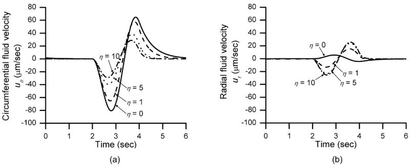
Parametric investigation of the leakage coefficient (η, defined in Appendix B) on canalicular fluid flow (a) in the circumferential direction and (b) in the radial direction at the FRAP sites (i.e., 30 μm below periosteum). Loading parameters include a peak force of 3 N, 2 sec per cycle, and 4 sec resting periods. The case of η = 0 corresponds to an impermeable boundary and η→∞ indicates a free flow boundary. The circumferential fluid velocity is found to be ∼10 times faster in the direction (u_θ) than in the radial direction (u_r), when the periosteum is relatively impermeable (η = 0, 1), and this difference diminishes as the periosteum becomes more leaky (η = 5, 10).

Three representative tracers that cover a spectrum of biological molecules found in bone (ions, nutrients, metabolites, hormones, cytokines, and proteins) are assumed to have diffusion coefficients in the LCS of 300, 30, or 3 μm²/sec. The diffusion coefficients of small molecules like sodium fluorescein were recently measured in mouse tibia to be on the order of 300 μm²/sec.⁴⁶ Those of larger molecules have not been quantified in bone but have been measured on the order of 3-10 μm²/sec in cytoplasma⁵⁶ and cartilage matrix.⁵⁷ Transport of these molecules during FRAP in the LCS of loaded bone is assumed to follow a modified diffusion-convection equation:

$$\frac{\partial C}{\partial t}+\left(1-{\sigma }_f\right)u\frac{\partial C}{\partial x}=D\frac{{\partial }^{2}C}{\partial x^2}$$ (Eq. 5)

where C(x, t) is the tracer concentration, t is the time after photobleaching, x is the linear coordinate of the position, σ_f is the tracer reflection coefficient that accounts for the molecular sieving from the pericellular matrix on the velocity of solutes, u(x, t) is the convective fluid flow velocity that varies spatially along the flow path, and D is the diffusion coefficient of the tracer. In the canaliculi sets (C₁ and C₂), the fluid velocity u(x, t) equals the opposite of the circumferential flow velocity (−u_θ), which has been calculated from the whole bone model (Eq. 4).

This model differs from the previous ones^36-41 by considering the reduction of the solute velocity due to the pericellular fiber matrix in the flow pathway. The solute movement lags behind the fluid by a factor of (1-σ_f), with greater reductions experienced by larger molecules. Since there are no available data on the reflection coefficients in bone, we adapt a model developed for endothelial glycocalyx⁵⁸ and estimate σ_f to be 0.84, 0.36 and 0.015 for the three representative tracers with diffusion coefficients of 3, 30 and 300 μm²/sec in the LCS.

The tracer movement after photobleaching the central lacuna follows Eq. 5 and is subjected to the following boundary and initial conditions, such as i) constant tracer concentrations at the two reservoirs at either side of the photobleached lacuna (C = C₀); ii) an initial 50% photobleaching of the central lacuna (C_b = 0.5C₀); and iii) initial linear concentration distribution in other regions, due to the relatively slow bleaching process.⁴⁶

To obtain the temporal and spatial distribution of the tracer profiles, Eq. 5 and the boundary and initial conditions are first rendered dimensionless as detailed in Appendix C. The LCS transport model (Fig. 3) is then digitized using a non-uniform mesh, with a more refined mesh placed on the tapered section where the velocity gradients are greater. Although the geometry is symmetric, the entire model is meshed and used in the calculation due to the anti-symmetric nature of the oscillating flow in the two canalicular sets (C₁ and C₂). A finite difference scheme (modified total variation diminishing Lax-Friedrichs method)⁵⁹ is implemented in Matlab (Mathworks, MA) to calculate tracer transport for varying mechanical loading conditions as given in the preceding section.

The model input is the fluid velocity u(x,t) predicted from the tissue-level mechanics model. The model output is the tracer concentration profile C(x,t), from which several characteristics of the solute flows are calculated, including the recovery rate (the slope magnitude of the curve of ln [(C − C₀)/(C_b − C₀)]) versus time), the Peclet number $[\text{Pe}=\left(1-{\sigma }_f\right)\frac{u_{0}d}{D}]$ that describes the relative effects of convection and diffusion (characterized by the maximal solute velocity in canaliculi (1-σ_f)u₀, and diffusion coefficient D, respectively), and the Strouhal number (St) that describes the effect of flow oscillation over the mean flow. The St number (St = d/d_ss).represents the ratio of the characteristic transport length (the canalicular length d) over the maximal displacement that the solute front travels during oscillation (termed as the solute stroke displacement d_ss). The solute stroke displacement $(d_{ss}=2t_2\left(1-{\sigma }_f\right)u_0/\pi +2\sqrt{D{t}_1})$ consists of solute front movement due to both convection during the half of a loading cycle (t₂, the first term) and diffusion during the half of a resting period (t₁, the second term).

Results

The default loading parameters for the results presented below, if not specified otherwise, are 3N peak force (F), 2 sec loading period (2t₂), and 4 sec resting period (2t₁). In some cases, the loading parameters are varied for the peak force (F = 0.3 to 3.5 N) and the loading period (2t₂ = 0.2 to 4 sec) while the resting period is kept constant (2t₁ = 4 sec). Three representative (small, medium, large) tracers with diffusion coefficients of 300, 30, and 3 μm²/sec in the LCS are chosen in most cases presented below. Three additional tracers with diffusion coefficients of 100, 60 and 10 μm²/sec are adopted when the effects of diffusion coefficient on FRAP recovery rate are studied.

Canalicular Fluid Velocities

The canalicular fluid velocity at the FRAP site is found to be approximately ten times faster in the circumferential direction (u_θ) than in the radial direction (u_r), when the periosteum is relatively impermeable (η = 0, 1), and this difference diminishes as the periosteum becomes more leaky as shown in the parametric study (η = 5, 10, Fig. 4). When the murine tibia is subjected to an end loading of a 3 N peak force, over a two second sinusoidal loading cycle with a four second resting period for imaging, the peak circumferential velocity at the FRAP site decreases from ∼80, 65, 40, to 30 μm/sec when the leakage coefficient η increases from 0, 1, 5, to 10 (Fig. 4a). In contrast, the corresponding radial velocity at the FRAP location increases from ∼5, 15, 24, to 26 μm/sec (Fig. 4b). Similar patterns are found for other loading conditions of peak load (0.3-3.5 N) and of loading periods (0.2-4 sec). However, we expect that the periostem remains relatively impermeable around our FRAP area, based on that fact that the periosteum near the FRAP region of interest is typically devoid of muscle attachment, and thus has fewer penetrating vessels compared to other anatomical locations. Furthermore, we can select lacunae away from any existing vessels or open channels during our studies to justify the simplification of the one-dimensional transport model, where only the circumferential, but not the radial, flow is considered (Fig. 3).

Tracer Concentration Profiles in LCS

The transport model clearly demonstrates that the load-induced oscillating flows reduce the diffusion distance and enhance the tracer refilling in the photobleached lacuna (Fig. 5). The temporal evolution of the spatial tracer profiles along the entire LCS fluid pathway exhibits three distinct phases of the tracer transport:

Fig. 5.

Spatial-temporal profiles of tracer concentration in the bone LCS during cyclic loading. The loading parameters include 3 N peak force, 2 sec load period, 2 sec resting period before and after loading. The resulting canalicular fluid waveform (with a maximal velocity of 81 μm/sec) and the examined time points are given in the first column. A positive fluid velocity indicates that fluid moves from the left reservoir towards the right. The tracer profiles for the three tracers with diffusion coefficients of 300, 30, and 3 μm²/sec are presented for the first oscillation cycle at the corresponding time points. Minimized transport models are placed on the top of the figure showing the spatial locations of the photobleached lacuna and the two canalicular sets. Two vertical broken lines in the tracer profiles indicate the junctions of the photobleached lacuna and the canaliculi. The concentration profiles show three distinct transport phases, including the initial diffusion phase (t = 0-2 sec) with no flow, the flow phase (t = 2-3.25 sec), and the reverse flow phase (t = 3.25-6 sec). The mean tracer concentration in the central lacuna increases more quickly during the last two phases due to convection of high concentrated solutes from the reservoirs into the photobleached lacuna, especially for the smaller tracers.

1) Diffusion phase (t = 0-2 sec): diffusion from both reservoirs slightly increases the concentration in the central lacuna. The tracer concentration profiles in the canaliculi remained approximately linear for the three tracers. 2) Flow phase (t = 2-3.25 sec): Fluid moves from the left reservoir towards the central lacuna once the load is applied. High-concentrated fluid begins to move towards the central lacuna and effectively reduces the transport distance between the source and sink, compared with that during diffusion (the canalicular length d). Simultaneously, the low-concentrated fluid is pushed out of the central lacuna towards the right reservoir. As a result, the mean concentration in the central lacuna increases for the three tracers. 3) Reverse flow phase (t = 3.25-6 sec): As the flow reverses its direction, high-concentrated fluid moves from the right reservoir towards the central lacuna. Meanwhile, the outflow from the central lacuna pushes away some of the high concentrated fluid that still remains at the left canaliculi set. This outflow seems to counteract the inflow and thus has a negative effect on the net transport into the lacuna, especially for large tracers with slower mixing. Although the fluid velocity u remains the same for all three tracers, they move at different speeds due to their varying molecular size and reflection coefficients, i.e., 0.985u, 0.64u, 0.16u, for the small, medium, and large tracer, respectively. As a result, the total influx volume during a half of the oscillation cycle is greater for the smaller tracer, resulting in a faster refilling rate. At the end of the cycle, the concentration profiles for the larger molecules are less smooth. The same process repeats itself throughout the subsequent loading cycles.

Recovery Rate for Tracer Refilling in the Photobleached Lacuna

The tracer refilling in the photobleached lacuna is found to follow an exponential damping process with a constant rate k, which is determined by the applied loading and tracer size (Fig. 6). The slopes of the logarithmic recovery ratio (ln [(C − C₀)/(C_b − C₀)]) versus time curves are steeper during loading periods (t = 2-4, 8-10, 14-16 sec) than during resting periods, indicating faster tracer refilling. A linear relationship is found among the hypothetical experimental data captured during the resting periods, suggesting an overall damping process that can be represented by C_sn = e^−kt_n, where C_sn is the recovery ratio after the nth loading cycle, t_n is the corresponding time point, and k is the overall recovery rate. We find that the recovery rate is increasing for decreasing tracer size (i.e., 0.00034, 0.0075, and 0.028 sec^-1 for the small, medium and large tracers, respectively, Fig. 6). We further investigate how the recovery rate is influenced by the tracer diffusion (or size), loading magnitude, and loading period.

Fig. 6.

The logarithmic recovery of tracer refilling in the photobleached lacuna for different tracers. The canalicular fluid velocity waveforms induced by a loading of 3 N peak force, 2 sec loading period, and 4 sec resting period are shown at the top of the figure. The vertical axis represents the logarithm of tracer recovery (C-C₀) relative to the initial photobleaching depth (C-C_b). The slopes of the logarithmic recovery ratio curves reflect the speeds of tracer refilling. Recovery is much faster (as seen in the steeper slopes) during loading intervals than the resting periods. The overall recovery rates, which are defined as the slopes of the straight lines that connect the hypothetical experimental data measured during resting periods (indicated with square, circle, and triangles for the large, medium and small tracers), increase with increasing diffusion coefficients.

Effects of the Tracer Size on the Recovery Rate

The recovery rate k increases monotonically with increasing diffusion coefficients, decreasing molecular size (and reflection coefficient) (Fig. 7a). When compared to the pure diffusion recovery rate (k₀), which is calculated for each tracer by setting convection flow to be zero, mechanical loading is found to increase transport of all tracers as the transport enhancement (the ratio of recovery rates between loaded versus non-loaded condition, k/k₀) is greater than 1 (Fig. 7b). However, the greatest enhancement is found for medium-sized tracers with a diffusion coefficient of 30 μm²/sec and less enhancement for small and large tracers (Fig. 7b).

Fig. 7.

Effects of the tracer diffusion coefficient (tracer size) on tracer transport. (a) The tracer recovery rate k increases with increasing diffusion coefficient. (b) Compared to diffusion (k₀), mechanical loading induces larger enhancement in transport of medium-sized molecules while a relatively smaller enhancement in transport of larger molecules with smaller diffusion coefficients (due to higher reflection coefficients) and smaller molecules with larger diffusion coefficients (due to faster diffusion baselines).

Effects of the Loading Magnitude on Recovery Rate

The recovery rate k increases with increasing peak force (F) and decreasing tracer size, when loading and resting periods remain to be 2 and 4 sec, respectively (Fig. 8a). The overall recovery rate k decreases with the increasing Strouhal number for the three tracers, which can be well fit with an inverse power law function (k = 0.003*St^-2.14) with a R² of 0.96 (Fig. 8b). The recovery rate shows two distinct patterns dictated by the St number. Slower transport (k < 0.0025 sec^-1) occurs for the cases of St > 1 and transport increases much more rapidly for the cases of St < 1 (Fig. 8b). The case of St = 1 corresponds to a solute stroke displacement (d_ss) equal to the distance between the reservoir and the photobleached lacunae d.

Fig. 8.

Effects of the loading magnitude on tracer transport. (a) The overall recovery rate k increases with increasing peak force F and increasing diffusion coefficients. (b) A reverse power law relationship exists between the overall recovery rate k and the Strouhal number St and two totally different transport regions occur for cases of St < 1 (rapid transport) and St > 1 (slow transport). The critical value of St = 1 corresponds the case when the stroke displacement for the tracers equals the canalicular length during the half oscillating cycle.

Effects of the Loading Period on Recovery Rate

The overall recovery rate k increases with increasing loading period (2t₂) up to around 2 seconds where it levels off for larger molecules and slightly decreases for smaller molecules (Fig. 9a). Similar to the loading magnitude effects, the recovery rate k follows a similar inverse power law relationship with St (k = 0.003*St^-2) and displays the same two distinct patterns above and below St = 1 (Fig. 9b).

Fig. 9.

Effects of the loading period on tracer transport. (a) The overall recovery rate k increases with increasing loading period (2t₂) up to around 2 seconds where it leveled off for larger molecules and slightly decreased for smaller molecules. (b) A nearly identical inverse power law relationship exists between the overall recovery rate k and the Strouhal number St, with two totally different transport behaviors for St < 1 and St > 1.

Discussion

The most important finding from the present model is that the behavior of solute flows in the LCS under an intermittent cyclic loading is determined by the dimensionless Strouhal (St) number that describes the relative effect of flow oscillation versus mean flow (Figs. 8 and 9). We also investigate the Peclet number, but fail to find a clear correlation between it and the recovery rate (data not shown). The possible explanation is that while Peclet number better characterizes uni-directional flows, it is the Strouhal number that captures the physics of oscillating flows.^60-63 In our study, we define the Strouhal number as the ratio of the characteristic transport length (the canalicular length) over the stroke displacement of the solute front during the load-induced flow oscillation. We find a nearly identical inverse power law relationship between the recovery rate and St number (k = 0.003*St^-2.14 or k = 0.003*St^-2) when the loading magnitude or frequency are varied (Figs. 8 and 9). We suspect that the powers and the constants in the power law relationships between k and St are dependent on the LCS anatomic features, which is under further investigations. The current results from the model clearly demonstrate two dramatically different transport behaviors when the St is above or below 1 (Fig. 8b). This result suggests a mechanical mechanism that accounts for the enhancement of load-induced transport in bone. This enhancement is due to tracer influx into the photobleached lacuna when the stroke displacement for the solute equals or exceeds the distance between the reservoir and the photobleached lacunae d. This threshold phenomenon is similar to the mixing threshold proposed in our previous osteon model.³⁹ The fundamental difference is that the earlier model neglects molecular sieving from the pericellular matrix and assumes large solutes move at the same speed as the fluid.³⁹ In contrast, the present model considers a reduction of solute speed due to the drag effects (reflection coefficients) from the pericellular matrix (Eq. 5). The reflection coefficients for the three tracers are estimated using an endothelial glycocalyx model,⁵⁸ since there are no reported values in bone. We may need to adjust these reflection coefficients when their experimental measurements are available in the future. Nevertheless, the model's prediction that solute transport behaves differently for the ranges of St >1 and St <1 will still hold true.

The model elucidates several general behaviors of tracer refilling in a loaded bone. The rate of fluorescence recovery after photobleaching is found to be greatly enhanced by applying an intermittent mechanical loading to the whole bone, and this enhancement is especially pronounced for higher loading magnitudes (Fig. 8) and lower loading frequencies (Fig. 9). These results are qualitatively comparable with the previous models,^{39, 43} and can be explained using the dimensionless St number. Higher loading magnitudes decrease the St number by increasing the magnitudes of mean flow (u₀) that carries more solute influx into the photobleached lacunae, resulting in more rapid tracer refilling (Fig. 8). The model also shows that increasing the loading period (i.e., lower loading frequency) will decrease the St number, leading to a faster recovery rate for all the tracers (Fig. 9). Moreover, our results provide quantitative information about the transport enhancement due to convection for various tracers. This notion has been suggested in many previous studies,^{10, 36, 38, 39} and a small transport enhancement (∼1.32) was found for a small tracer (D = 300 μm²/sec) under a loading of ∼100 micronstrain and 2 Hz.⁷¹ Our results show that, while convective enhancement occurs for all the tracers examined in this study (k/k₀ >1), the most pronounced enhancement happens for the medium-sized tracers and a relatively smaller enhancement is found for either small or large tracers (Fig. 7b). The reason for this bi-phasic behavior is that the small tracers have relatively fast baseline diffusions that diminish the contribution of convection to the total transport, while the large tracers have high tracer reflections in the pericellular matrix that reduce the convective transport itself.

The present study provides guidelines for future experimental measurement of fluid and solute flows in bone. First of all, this model validates the use of intermittent loading since it confirms that enhanced tracer refilling can be achieved. Qualitatively, the model suggests that higher loading magnitudes at lower frequencies would result in a higher load-induced transport enhancement, especially for medium-sized tracers. These optimized parameters can be used to increase the sensitivity of detecting such effects in the experiments. Secondly, the model suggests a straightforward method for data analysis by envisioning transport in FRAP experiments as an exponential damping process that is characterized by a single parameter, the overall recovery rate k, (Fig. 6). This is similar to the case of pure diffusion of small molecules in our previous FRAP experiments.⁴⁶ The overall recovery rate k can be readily obtained from the FRAP experimental data to quantify and compare transport efficiency at different loading magnitudes, frequencies, and for various molecules. Lastly, the model provides a tool to obtain the LCS permeability, solute-matrix interactions and quantitative measures of fluid and solute flows from experimental data. The two important parameters in the model are the characteristic relaxation time τ_r that determines the fluid flow (e.g., maximal velocity u₀, and velocity profile) and the reflection coefficient of the solute that determines the solute flow. Both parameters are currently estimated using mathematical models and their values are shown to be sensitive to the model parameters.^{9, 39, 54, 58, 64} To experimentally determine these important parameters, FRAP experiments can be performed for various tracers with different loading magnitudes. The derived recovery rates k_e will be used to find the best fit characteristic relaxation time and reflection coefficient using optimization methods such as the simulated annealing algorithm.⁶⁵ Once these two critical parameters are determined, the St number and the fluid and solute velocities can be readily obtained for each loading condition using the model.

Although the present study focuses on fluid and solute transport that occurs at a specific location, 30 μm beneath the periosteum and for a particular loading regimen, the equations and methods can be used to study fluid and solute flows at other locations and for other loading waveforms. Fluid and solute flows at the inner and outer bone surfaces are of more physiological importance because they present the largest stimuli for the osteocytes and provide signaling to cells lining the surfaces.⁶⁶ The order of the flow magnitudes in an arbitrary position can be estimated from the flow at the FRAP location. Flows at other circumferential positions will be no greater than the FRAP site because of their corresponding lower loading rates (Eq. 3). For the radial flow at the bone endosteum, previous models have shown that its magnitude may be 10-30 times higher than the radial flow close to the periosteum.^{42, 66} Therefore, it is reasonable to predict that the peak radial flow at the endosteum is at the same order of magnitude as the circumferential peak flow velocity at the FRAP site, ∼80 μm/sec for a 800 microstrain loading that is used in the current model (Fig. 4).

There are several limitations and assumptions in the current study. First, idealized poroelastic and transport models are used to simplify the mathematics, although the murine tibia is of a triangular shape, and the anatomical features of the LCS are expected to vary in vivo. Secondly, the bone tissue is assumed to have isotropic mechanical properties and LCS permeability. Intracortical porosity, which has been shown in previous studies to influence the local drainage of fluid,^{67, 68} is neglected in the tibial cross-section, because few intracortical pores are found in the thin cortex of the mouse strain used in the experiments.⁶⁹ In addition, one-dimensional transport is assumed by considering the circumferential flow and neglecting the radial flow, which is valid only when the periosteum is relatively impermeable as expected around the FRAP regions. If future data suggest an otherwise more leaky periosteum, the radial flows have to be considered. The extracellular fluid space in the lacuna is also assumed to remain constant along the long axis of the lacuna. Lastly, only an intermittent loading waveform is considered, although the method described could be used for other waveforms using Fourier transform.

Despite its limitations, the current model provides a more accurate description of solute convection in loaded bone by incorporating the coupling of bone mechanics with solute transport at the tissue and cellular levels and by considering the effects of pericellular matrix on both fluid and solute flows. Most importantly, this model finds that the fundamental dimensionless number, the Strouhal number, controls the solute flows, and defines a threshold mechanism that accounts for the both convective and diffusive transport in the LCS. This model also has a potential application to quantify intrinsic properties of bone such as LCS permeability and the tracer reflection coefficient through the pericellular matrix. In addition, the model provides guidelines for designing experiments and a framework for their analysis. The detailed knowledge of load-induced fluid and solute flows is essential for our understanding of the mechanosensation, metabolism, signaling pathways of osteocytes, which have recently been found to play important regulatory roles in bone physiology, and for designing new pharmaceutical agents and delivery systems for treating various bone diseases such as osteoporosis and osteonecrosis.

Appendix A. Estimation of the LCS permeability and the characteristic fluid relaxation time

The hydraulic permeability of a single canaliculus k_p has been estimated using a model of rectangular lattice of transverse fibers in the fluid field.⁹

$$k_p=0.0572a_0^2{\left(\Delta /a_0\right)}^{2.377},$$ (Eq. A1)

where a₀ is the radius of the pericellular fibers (assumed to that of proteoglycan GAG side chain, 0.6nm), and Δ is the effective spacing of the fibers of the pericellular matrix (7 nm).

The tissue level permeability k is estimated from the anatomical features of the LCS, assuming a regular array of osteocytes and homogenous canalicular distribution as in Weinbaum et al. (1994):

$$k=\frac{2\pi N{a}^4{q}^3}{6{\gamma }^3{d}^2}\left\{A_1\left[I_1\left(\gamma /q\right)-q{I}_1\left(\gamma \right)\right]+B_1\left[q{K}_1\left(\gamma \right)-K_1\left(\gamma /q\right)\right]+\frac{\gamma \left(q^2-1\right)}{2q}\right\},$$ (Eq. A2)

where a is the radius of the osteocyte process, q is the ratio of the radius of the canaliculus (b) to the radius of the osteocytic process (a), d is the average spacing between two lacunae, N is the total number of canaliculi emanating from one lacuna, γ is a dimensionless length ratio between the canalicular radius and its associated boundary layer thickness, which is approximated to be the square root of the permeability of a single canaliculus $(\gamma =b/\sqrt{k_p})$. A₁ and B₁ are defined as

$$A_1=\frac{K_0\left(\gamma \right)-K_0\left(\gamma /q\right)}{I_0\left(\gamma /q\right)K_0\left(\gamma \right)-I_0\left(\gamma \right)K_0\left(\gamma /q\right)}$$ (Eq. A3)

$$B_1=\frac{I_0\left(\gamma /q\right)-I_0\left(\gamma \right)}{I_0\left(\gamma /q\right)K_0\left(\gamma \right)-I_0\left(\gamma \right)K_0\left(\gamma /q\right)}$$ (Eq. A4)

where I₀, K₀, I₁ and K₁ are modified Bessel functions of the first and second kind.

The characteristic fluid relaxation time is defined as:

$${\tau }_r=\frac{\mu r_o^2}{k\left(13.5\text{GPa}\right)}.$$ (Eq. A5)

where μ is the viscosity of bone fluid and assumed to be that of sea water (μ =1.06×10^-3 kg/(m·s)); r₀ is the radius of the periosteum. The value of τ_r is found to be 6.76 sec for the mid-shaft tibia of B6 mouse (r₀ = 0.57 mm) when the reported values of the LCS ultra- and micro-structures are used (i.e., a = 52 nm; b =130 nm; N = 70; d = 30 microns).³⁵, ⁴⁶ The sensitivity of τ_r on fiber spacing, size of cell process and canalicular wall was performed previously, and τ_r was found to be more sensitive to the fiber spacing.⁷⁰

Appendix B. Fluid pore pressure, pressure gradient, and canalicular fluid velocity

The intermittent dynamic force f(t) (see Fig. 1 and Eq. 1 in the text) can be expanded into a Fourier series:

$$f\left(t\right)=F\left(A_0+\sum _{n=1}^{\infty }{A}_n\text{cos}\frac{t}{t_1+t_2}n\pi \right),$$ (Eq. B1)

where F is the peak-to-peak force and 2t₁ is the resting time and 2t₂ is the loading period and the coefficient for each term is defined as:

$$A_0=-\frac{t_2}{2\left(t_1+t_2\right)},A_n={\left(-1\right)}^n\frac{{\left(t_1+t_2\right)}^2}{n\pi \left[n^2{t}_2^2-{\left(t_1+t_2\right)}^2\right]}\text{sin}\left(\frac{n\pi t_2}{t_1+t_2}\right).$$ (Eq. B2)

Using a set of parameters [R = r/r_o ; τ = t/τ_r ; T = ωτ_r ; ω = π/(t₁ + t₂) ; and P = 3pA/(BTF)] and substituting the Fourier series of loading f(t), the poroelastic equation of the fluid pore pressure (Eq. 3 in the text) is rendered dimensionless:

$$\frac{{\partial }^{2}P}{\partial R^2}+\frac{1}{R}\frac{\partial P}{\partial R}+\frac{1}{R^2}\frac{{\partial }^{2}P}{\partial {\theta }^2}-\frac{\partial P}{\partial \tau }=-\left[1+\frac{L{r}_{o}A}{I}R\text{sin}\theta \right]\sum _{n=1}^{\infty }n{A}_n\text{sin}\left(nT\tau \right)$$ (Eq. B3)

where R, τ, T, and P are dimensionless radial position, time, frequency, and pressure respectively; ω is the principle angular loading frequency; F is the peak force of the dynamic loading; A is the cross-sectional area of the tibial mid-shaft, B is the Skempton parameter indicating the relative compressibility between the fluid and solid phases in bone (B = 0.53);⁵², ⁵³ r₀ is the exterior radius of the tibial mid-shaft, L is the offset of the loading force to the center of the bone, I is the moment of inertia of the bone cross-section along the medial-lateral axis, and A_n are the coefficients in the Fourier expansion (Eq. B2).

The boundary conditions are zero pressure at the inner endosteal surface and a leaky outer periosteal surface (Eq. 7), as in previous models³⁹, ⁴², ⁹:

$$P=0\text{at}R=\lambda =r_i/r_o;\frac{\partial P}{\partial R}+\eta P=0\text{at}R=1$$ (Eq. B4)

where η is the coefficient with η = 0 corresponding to no leakage condition and η→∞ corresponding to free flow.

The analytical solution of dimensionless pressure is derived using complex function and separate variables as follows:

$$\begin{array}{c}P\left(R,\theta ,\tau \right)=\sum _{n=1}^{\infty }\text{Im}\{[\frac{A_n}{iT}\left(1+\frac{L{r}_{o}A}{I}R\text{sin}\theta \right)+C_{0n}{I}_0\left(\sqrt{\text{inT}}R\right)+D_{0n}{K}_0\left(\sqrt{\text{inT}}R\right)\hfill \\ +\left(C_{1n}{I}_1\left(\sqrt{\text{inT}}R\right)+D_{1n}{K}_1\left(\sqrt{\text{inT}}R\right)\right)\text{sin}\theta ]e^{\text{inT}\tau }\}\hfill \end{array}$$ (Eq. B5)

where

$$C_{0n}=\frac{A_n}{\text{iT}}\frac{\sqrt{\text{inT}}{K}_1\left(\sqrt{\text{inT}}\right)-\eta \left[K_0\left(\sqrt{\text{inT}}\right)-K_0\left(\lambda \sqrt{\text{inT}}\right)\right]}{I_0\left(\lambda \sqrt{\text{inT}}\right)\left[\sqrt{\text{inT}}{K}_1\left(\sqrt{\text{inT}}\right)-\eta K_0\left(\sqrt{\text{inT}}\right)\right]+K_0\left(\lambda \sqrt{\text{inT}}\right)\left[\sqrt{\text{inT}}{I}_1\left(\sqrt{\text{inT}}\right)+\eta I_0\left(\sqrt{\text{inT}}\right)\right]}$$ (Eq. B6)

$$D_{0n}=\frac{A_n}{\text{iT}}\frac{\sqrt{\text{inT}}{I}_1\left(\sqrt{\text{inT}}\right)+\eta \left[I_0\left(\sqrt{\text{inT}}\right)-I_0\left(\lambda \sqrt{\text{inT}}\right)\right]}{I_0\left(\lambda \sqrt{\text{inT}}\right)\left[\sqrt{\text{inT}}{K}_1\left(\sqrt{\text{inT}}\right)-\eta K_0\left(\sqrt{\text{inT}}\right)\right]+K_0\left(\lambda \sqrt{\text{inT}}\right)\left[\sqrt{\text{inT}}{I}_1\left(\sqrt{\text{inT}}\right)+\eta I_0\left(\sqrt{\text{inT}}\right)\right]}$$ (Eq. B7)

$$C_{1n}=-\frac{A_{n}L{r}_{o}A}{\text{iIT}}\frac{\lambda \left[\sqrt{\text{inT}}{K}_0\left(\sqrt{\text{inT}}\right)+\left(1-\eta \right)K_1\left(\sqrt{\text{inT}}\right)\right]+\left(1+\eta \right)K_1\left(\lambda \sqrt{\text{inT}}\right)}{I_1\left(\lambda \sqrt{\text{inT}}\right)\left[\sqrt{\text{inT}}{K}_0\left(\sqrt{\text{inT}}\right)+\left(1-\eta \right)K_1\left(\sqrt{\text{inT}}\right)\right]+\left[\sqrt{\text{inT}}{I}_0\left(\sqrt{\text{inT}}\right)-\left(1-\eta \right)I_1\left(\sqrt{\text{inT}}\right)\right]K_1\left(\lambda \sqrt{\text{inT}}\right)}$$ (Eq. B8)

$$D_{1n}=-\frac{A_{n}L{r}_{o}A}{\text{inT}}\frac{\lambda \left[\sqrt{\text{inT}}{I}_0\left(\sqrt{\text{inT}}\right)-\left(1-\eta \right)I_1\left(\sqrt{\text{inT}}\right)\right]-\left(1+\eta \right)I_1\left(\lambda \sqrt{\text{inT}}\right)}{I_1\left(\lambda \sqrt{\text{inT}}\right)\left[\sqrt{\text{inT}}{K}_0\left(\sqrt{\text{inT}}\right)+\left(1-\eta \right)K_1\left(\sqrt{\text{inT}}\right)\right]+\left[\sqrt{\text{inT}}{I}_0\left(\sqrt{\text{inT}}\right)-\left(1-\eta \right)I_1\left(\sqrt{\text{inT}}\right)\right]K_1\left(\lambda \sqrt{\text{inT}}\right)}$$ (Eq. B9)

The gradients of the dimensionless pressure in the radial and circumferential directions are obtained from Eq. B5:

$$\begin{array}{c}\frac{\partial P}{\partial R}=\sum _{n=1}^{\infty }\text{Im}\{[\frac{A_{n}L{r}_{o}A}{\text{iIT}}\text{sin}\theta +C_{0n}\sqrt{\text{inT}}{I}_1\left(\sqrt{\text{inT}}R\right)-D_{0n}\sqrt{\text{inT}}{K}_1\left(\sqrt{\text{inT}}R\right)\hfill \\ +\left(C_{1n}\sqrt{\text{inT}}{I}_0\left(\sqrt{\text{inT}}R\right)+\frac{C_{1n}}{R}{I}_1\left(\sqrt{\text{inT}}R\right)-D_{1n}\sqrt{\text{inT}}{K}_0\left(\sqrt{\text{inT}}R\right)-\frac{D_{1n}}{R}{K}_1\left(\sqrt{\text{inT}}R\right)\right)\text{sin}\theta ]e^{\text{inT}\tau }\}\hfill \end{array}$$ (Eq. B8)

$$\frac{\partial P}{\partial \theta }=\sum _{n=1}^{\infty }\text{Im}\left\{\left[\frac{A_n}{iT}\frac{L{r}_{o}A}{I}R\text{cos}\theta +\left(C_{1n}{I}_1\left(\sqrt{\text{inT}}R\right)+D_{1n}{K}_1\left(\sqrt{\text{inT}}R\right)\right)\text{cos}\theta \right]e^{\text{inT}\tau }\right\}$$ (Eq. B9)

The corresponding canalicular fluid velocities in the radial and circumferential directions are derived using Darcy's law:

$$u_r=-\frac{k_p}{\mu }\frac{\partial p}{\partial r}=-\frac{k_p\text{BTF}}{3\mu r_{o}A}\frac{\partial P}{\partial R}$$ (Eq. B10)

$$u_{\theta }=-\frac{k_p}{\mu r}\frac{\partial p}{\partial \theta }=-\frac{k_p\text{BTF}}{3\mu \text{rA}}\frac{\partial P}{\partial \theta }$$ (Eq. B11)

where p is the fluid pressure, P is the dimensionless pressure, and k_p is the permeability of a single canaliculus (defined in Eq. A1 in Appendix A).

Appendix C. Unified Transport Equation for the Bone LCS

For the three-compartment transport model (shown in Fig. 3 in the text), oscillating fluid and solute flows occur in the idealized one-dimensional LCS pathway with varying cross-sectional area. A unified, compact form of the transport equation for all segments is derived here. A liner x coordinate is defined and originated from the central lacuna (Fig. 3).

In canaliculi (d_e + d_s ≤ |x| ≤ d + d_e + d_s)

The solute transport satisfies the modified diffusion-convection equation through a porous media

$$\frac{\partial C}{\partial t}+\left(1-{\sigma }_f\right)u\frac{\partial C}{\partial x}=D\frac{{\partial }^{2}C}{\partial x^2},$$ (Eq. C1)

where C is the tracer concentration, u is the bulk flow velocity (- u_θ in this case), and D is the diffusion coefficient of the tracer. The boundary conditions are

$$C\left(\pm \left(d+d_e+d_s\right),t\right)=C_0,$$ (Eq. C2)

where C₀ is the tracer concentration that remains constant in the two source reservoirs. Initially, a linear distribution is assumed in the canaliculi connecting the reservoir and the photobleached lacuna, assuming a relative slow photobleaching process.⁴⁶

$$C\left(x,0\right)=C_0+\left(C_b-C_0\right)\frac{d_s+d_e+d-\left|x\right|}{d},$$ (Eq. C3)

where C_b is the concentration inside the photobleached lacuna immediately after photobleaching.

Tapered Entrance (d_s ≤ |x| ≤ d_e + d_s)

The connection between the canalicular channels and the photobleached lacuna is modeled as a tapered tube with expanding cross-sectional area. The cross-sectional area is a function of position x as:

$$A={\left(1+\beta \frac{d_s+d_e-\left|x\right|}{d}\right)}^2{A}_c,$$ (Eq. C4)

where A_c is the summation of the cross-sectional area of the connecting canaliculi. The expansion factor β describes the cross-section radius increment on unit axial distance. Since the tapered entrance connects with the lacuna at the other end, (A = A_f, extracellular fluid space in the lacuna, when |x| = d_s), β can be determined by

$$\beta =\frac{d}{d_e}\left(\sqrt{A_f/A_c}-1\right)$$ (Eq. C5)

The flow velocity in this section decreases with the increasing cross-sectional area:

$$u_{\text{exp}}=\frac{u}{{\left(1+\beta \frac{d_s+d_e-\left|x\right|}{d}\right)}^2}.$$ (Eq. C6)

The solute conservation equation is

$$A\frac{\partial C}{\partial t}+\left(1-{\sigma }_f\right)u_{\text{exp}}A\frac{\partial C}{\partial x}=D\frac{\partial }{\partial x}\left(A\frac{\partial C}{\partial x}\right),$$ (Eq. C7)

After substituting Eqs. C6 and C4 into Eq. C7, we derive the following equation for tapered section:

$$\frac{\partial C}{\partial t}+\left\{\frac{\left(1-{\sigma }_f\right)u}{{\left[1+\beta \left(d_s+d_e-\left|x\right|\right)/d\right]}^2}+\frac{2\text{sgn}\left(x\right)D\beta /d}{1+\beta \left(d_s+d_e-\left|x\right|\right)/d}\right\}\frac{\partial C}{\partial x}=D\frac{{\partial }^{2}C}{\partial x^2}.$$ (Eq. C8)

The initial condition for this section is that it is photobleached as the overall lacuna, i.e.,

$$C\left(x,0\right)=C_b.$$ (Eq. C9)

Photobleached lacuna (|x| ≤ d_s)

Assuming the cross-sectional area of the extracellular fluid space in the lacuna (A_f) remains constant along its long axis, A_f can be obtained from Eq. C5 as

$$A_f={\left(1+\beta \frac{d_e}{d}\right)}^2{A}_c={\left(1+\beta {\lambda }_2\right)}^2{A}_c,$$ (Eq. C10)

where ${\lambda }_2=\frac{d_e}{d}$. Therefore, the fluid velocity in this region will decrease and the convection-diffusion equation becomes

$$\frac{\partial C}{\partial t}+\frac{\left(1-{\sigma }_f\right)u}{{\left(1+\beta {\lambda }_2\right)}^2}\frac{\partial C}{\partial x}=D\frac{{\partial }^{2}C}{\partial x^2}.$$ (Eq. C11)

The initial condition is that the entire of the lacuna will be uniformly photobleached as follows:

$$C\left(x,0\right)=C_b.$$ (Eq. C12)

Unified dimensionless equation

The above equations can be rendered dimensionless using the following dimensionless parameters (Eq. C13).

$$x^{\ast }=\frac{x}{d},\tau =\frac{d^2}{D},t^{\ast }=\frac{t}{\tau },C^{\ast }=\frac{C-C_0}{C_0},\text{Pe}=\left(1-{\sigma }_f\right)\frac{u_{0}d}{D},u^{\ast }=\frac{u}{u_0},{\lambda }_1=\frac{d_s}{d},{\lambda }_2=\frac{d_e}{d}$$ (Eq. C13)

To obtain a compact form of the transport equations, we define two functions g and h that vary with spatial locations and reflect the influences of the cross-sectional area variation on convective velocity and mass flow rate:

$$g=\{\begin{array}{ll}1,\hfill & {\lambda }_1+{\lambda }_2\le \left|x^{\ast }\right|\le 1+{\lambda }_1+{\lambda }_2\left(\text{canaliculi}\right)\hfill \\ {\left[1+\beta \left({\lambda }_1+{\lambda }_2-\left|x^{\ast }\right|\right)\right]}^{-2},\hfill & {\lambda }_1\le \left|x^{\ast }\right|\le {\lambda }_1+{\lambda }_2\left(\text{taperedsections}\right)\hfill \\ {\left(1+\beta {\lambda }_2\right)}^{-2},\hfill & \left|x^{\ast }\right|\le {\lambda }_1\left(\text{photobleached lacuna}\right)\hfill \end{array}$$ (Eq. C14)

$$h=\{\begin{array}{ll}\frac{2\text{sgn}\left(x^{\ast }\right)\beta }{1+\beta \left({\lambda }_1+{\lambda }_2-\left|x^{\ast }\right|\right)},\hfill & {\lambda }_1\le \left|x^{\ast }\right|\le {\lambda }_1+{\lambda }_2\left(\text{taperedsections}\right)\hfill \\ 0,\hfill & \text{else}\hfill \end{array}$$ (Eq. C15)

The compact form of the transport equation is given as:

$$\frac{\partial C^{\ast }}{\partial t^{\ast }}+\left(\text{Pe}\cdot u^{\ast }\cdot g+h\right)\frac{\partial C^{\ast }}{\partial x^{\ast }}=\frac{{\partial }^2{C}^{\ast }}{\partial x^{\ast 2}}.$$ (Eq. C16)

The initial and boundary conditions are

$$C^{\ast }\left(\pm \left(1+{\lambda }_1+{\lambda }_2\right),t\right)=0,$$ (Eq. C17)

$$C^{\ast }\left(x,0\right)=\{\begin{array}{ll}\left(1+{\lambda }_1+{\lambda }_2-\left|x^{\ast }\right|\right)C_b^{\ast },\hfill & {\lambda }_1+{\lambda }_2\le \left|x^{\ast }\right|\le 1+{\lambda }_1+{\lambda }_2\left(\text{canaliculi}\right)\hfill \\ C_b^{\ast },\hfill & \left|x^{\ast }\right|\le {\lambda }_1+{\lambda }_2\left(\text{else}\right)\hfill \end{array}$$ (Eq. C18)

References

- 1.Takai E, Mauck RL, Hung CT, Guo XE. Osteocyte viability and regulation of osteoblast function in a 3D trabecular bone explant under dynamic hydrostatic pressure. J Bone Miner Res. 2004;19:1403–10. doi: 10.1359/JBMR.040516. [DOI] [PubMed] [Google Scholar]
- 2.Gross TS, King KA, Rabaia NA, Pathare P, Srinivasan S. Upregulation of osteopontin by osteocytes deprived of mechanical loading or oxygen. J Bone Miner Res. 2005;20:250–6. doi: 10.1359/JBMR.041004. [DOI] [PMC free article] [PubMed] [Google Scholar]
- 3.Rios HF, Ye L, Dusevich V, Eick D, Bonewald LF, Feng JQ. DMP1 is essential for osteocyte formation and function. J Musculoskelet Neuronal Interact. 2005;5:325–7. [PubMed] [Google Scholar]
- 4.Feng JQ, Ward LM, Liu S, Lu Y, Xie Y, Yuan B, Yu X, Rauch F, Davis SI, Zhang S, Rios H, Drezner MK, Quarles LD, Bonewald LF, White KE. Loss of DMP1 causes rickets and osteomalacia and identifies a role for osteocytes in mineral metabolism. Nat Genet. 2006;38:1310–5. doi: 10.1038/ng1905. [DOI] [PMC free article] [PubMed] [Google Scholar]
- 5.Robling AG, Niziolek PJ, Baldridge LA, Condon KW, Allen MJ, Alam I, Mantila SM, Gluhak-Heinrich J, Bellido TM, Harris SE, Turner CH. Mechanical stimulation of bone in vivo reduces osteocyte expression of Sost/sclerostin. J Biol Chem. 2007 doi: 10.1074/jbc.M705092200. [DOI] [PubMed] [Google Scholar]
- 6.Silvestrini G, Ballanti P, Sebastiani M, Leopizzi M, Di Vito M, Bonucci E. OPG and RANKL mRNA and protein expressions in the primary and secondary metaphyseal trabecular bone of PTH-treated rats are independent of that of SOST. J Mol Histol. 2007 doi: 10.1007/s10735-007-9158-6. [DOI] [PubMed] [Google Scholar]
- 7.Tatsumi S, Ishii K, Amizuka N, Li M, Kobayashi T, Kohno K, Ito M, Takeshita S, Ikeda K. Targeted ablation of osteocytes induces osteoporosis with defective mechanotransduction. Cell Metab. 2007;5:464–75. doi: 10.1016/j.cmet.2007.05.001. [DOI] [PubMed] [Google Scholar]
- 8.You L, Temiyasathit S, Lee P, Kim CH, Tummala P, Yao W, Kingery W, Malone AM, Kwon RY, Jacobs CR. Osteocytes as mechanosensors in the inhibition of bone resorption due to mechanical loading. Bone. 2008;42:172–179. doi: 10.1016/j.bone.2007.09.047. [DOI] [PMC free article] [PubMed] [Google Scholar]
- 9.Weinbaum S, Cowin SC, Zeng Y. A model for the excitation of osteocytes by mechanical loading-induced bone fluid shear stresses. J Biomech. 1994;27:339–60. doi: 10.1016/0021-9290(94)90010-8. [DOI] [PubMed] [Google Scholar]
- 10.Burger EH, Klein-Nulend J. Mechanotransduction in bone--role of the lacuno-canalicular network. Faseb J. 1999;13(Suppl):S101–12. [PubMed] [Google Scholar]
- 11.Klein-Nulend J, Semeins CM, Ajubi NE, Nijweide PJ, Burger EH. Pulsating fluid flow increases nitric oxide (NO) synthesis by osteocytes but not periosteal fibroblasts--correlation with prostaglandin upregulation. Biochem Biophys Res Commun. 1995;217:640–8. doi: 10.1006/bbrc.1995.2822. [DOI] [PubMed] [Google Scholar]
- 12.Westbroek I, Ajubi NE, Alblas MJ, Semeins CM, Klein-Nulend J, Burger EH, Nijweide PJ. Differential stimulation of prostaglandin G/H synthase-2 in osteocytes and other osteogenic cells by pulsating fluid flow. Biochem Biophys Res Commun. 2000;268:414–9. doi: 10.1006/bbrc.2000.2154. [DOI] [PubMed] [Google Scholar]
- 13.Poole KE, van Bezooijen RL, Loveridge N, Hamersma H, Papapoulos SE, Lowik CW, Reeve J. Sclerostin is a delayed secreted product of osteocytes that inhibits bone formation. Faseb J. 2005;19:1842–4. doi: 10.1096/fj.05-4221fje. [DOI] [PubMed] [Google Scholar]
- 14.Genetos DC, Kephart CJ, Zhang Y, Yellowley CE, Donahue HJ. Oscillating fluid flow activation of gap junction hemichannels induces ATP release from MLO-Y4 osteocytes. J Cell Physiol. 2007;212:207–14. doi: 10.1002/jcp.21021. [DOI] [PMC free article] [PubMed] [Google Scholar]
- 15.Bentolila V, Boyce TM, Fyhrie DP, Drumb R, Skerry TM, Schaffler MB. Intracortical remodeling in adult rat long bones after fatigue loading. Bone. 1998;23:275–81. doi: 10.1016/s8756-3282(98)00104-5. [DOI] [PubMed] [Google Scholar]
- 16.Verborgt O, Gibson GJ, Schaffler MB. Loss of osteocyte integrity in association with microdamage and bone remodeling after fatigue in vivo. J Bone Miner Res. 2000;15:60–7. doi: 10.1359/jbmr.2000.15.1.60. [DOI] [PubMed] [Google Scholar]
- 17.Duriez R, Duriez J. Periosteocyte demineralization in disuse osteoporsis. The effect of calcitonin. Int Orthop. 1981;5:299–304. doi: 10.1007/BF00271086. [DOI] [PubMed] [Google Scholar]
- 18.Dodd JS, Raleigh JA, Gross TS. Osteocyte hypoxia: a novel mechanotransduction pathway. Am J Physiol. 1999;277:C598–602. doi: 10.1152/ajpcell.1999.277.3.C598. [DOI] [PubMed] [Google Scholar]
- 19.Gross TS, Akeno N, Clemens TL, Komarova S, Srinivasan S, Weimer DA, Mayorov S. Selected Contribution: Osteocytes upregulate HIF-1alpha in response to acute disuse and oxygen deprivation. J Appl Physiol. 2001;90:2514–9. doi: 10.1152/jappl.2001.90.6.2514. [DOI] [PubMed] [Google Scholar]
- 20.Gluhak-Heinrich J, Ye L, Bonewald LF, Feng JQ, MacDougall M, Harris SE, Pavlin D. Mechanical loading stimulates dentin matrix protein 1 (DMP1) expression in osteocytes in vivo. J Bone Miner Res. 2003;18:807–17. doi: 10.1359/jbmr.2003.18.5.807. [DOI] [PubMed] [Google Scholar]
- 21.Burger EH, Klein-Nulend J, van der Plas A, Nijweide PJ. Function of osteocytes in bone--their role in mechanotransduction. J Nutr. 1995;125:2020S–2023S. doi: 10.1093/jn/125.suppl_7.2020S. [DOI] [PubMed] [Google Scholar]
- 22.Bloomfield SA. Cellular and molecular mechanisms for the bone response to mechanical loading. Int J Sport Nutr Exerc Metab. 2001;11(Suppl):S128–36. doi: 10.1123/ijsnem.11.s1.s128. [DOI] [PubMed] [Google Scholar]
- 23.Noble B. Microdamage and apoptosis. Eur J Morphol. 2005;42:91–8. doi: 10.1080/09243860500096248. [DOI] [PubMed] [Google Scholar]
- 24.Bonewald LF. Osteocytes as dynamic multifunctional cells. Ann N Y Acad Sci. 2007;1116:281–90. doi: 10.1196/annals.1402.018. [DOI] [PubMed] [Google Scholar]
- 25.Kufahl RH, Saha S. A theoretical model for stress-generated fluid flow in the canaliculi-lacunae network in bone tissue. J Biomech. 1990;23:171–80. doi: 10.1016/0021-9290(90)90350-c. [DOI] [PubMed] [Google Scholar]
- 26.Knothe Tate ML, Niederer P, Knothe U. In vivo tracer transport through the lacunocanalicular system of rat bone in an environment devoid of mechanical loading. Bone. 1998;22:107–17. doi: 10.1016/s8756-3282(97)00234-2. [DOI] [PubMed] [Google Scholar]
- 27.Qin YX, Lin W, Rubin C. The pathway of bone fluid flow as defined by in vivo intramedullary pressure and streaming potential measurements. Ann Biomed Eng. 2002;30:693–702. doi: 10.1114/1.1483863. [DOI] [PubMed] [Google Scholar]
- 28.Wang L, Ciani C, Doty SB, Fritton SP. Delineating bone's interstitial fluid pathway in vivo. Bone. 2004;34:499–509. doi: 10.1016/j.bone.2003.11.022. [DOI] [PMC free article] [PubMed] [Google Scholar]
- 29.Cooper RR, Milgram JW, Robinson RA. Morphology of the osteon. An electron microscopic study. J Bone Joint Surg Am. 1966;48:1239–71. [PubMed] [Google Scholar]
- 30.Cane V, Marotti G, Volpi G, Zaffe D, Palazzini S, Remaggi F, Muglia MA. Size and density of osteocyte lacunae in different regions of long bones. Calcif Tissue Int. 1982;34:558–63. doi: 10.1007/BF02411304. [DOI] [PubMed] [Google Scholar]
- 31.Marotti G, Remaggi F, Zaffe D. Quantitative investigation on osteocyte canaliculi in human compact and spongy bone. Bone. 1985;6:335–7. doi: 10.1016/8756-3282(85)90325-4. [DOI] [PubMed] [Google Scholar]
- 32.Marotti G, Ferretti M, Remaggi F, Palumbo C. Quantitative evaluation on osteocyte canalicular density in human secondary osteons. Bone. 1995;16:125–8. doi: 10.1016/s8756-3282(94)00019-0. [DOI] [PubMed] [Google Scholar]
- 33.Remaggi F, Cane V, Palumbo C, Ferretti M. Histomorphometric study on the osteocyte lacuno-canalicular network in animals of different species. I. Woven-fibered and parallel-fibered bones. Ital J Anat Embryol. 1998;103:145–55. [PubMed] [Google Scholar]
- 34.Ferretti M, Muglia MA, Remaggi F, Cane V, Palumbo C. Histomorphometric study on the osteocyte lacuno-canalicular network in animals of different species. II. Parallel-fibered and lamellar bones. Ital J Anat Embryol. 1999;104:121–31. [PubMed] [Google Scholar]
- 35.You LD, Weinbaum S, Cowin SC, Schaffler MB. Ultrastructure of the osteocyte process and its pericellular matrix. Anat Rec A Discov Mol Cell Evol Biol. 2004;278:505–13. doi: 10.1002/ar.a.20050. [DOI] [PubMed] [Google Scholar]
- 36.Piekarski K, Munro M. Transport mechanism operating between blood supply and osteocytes in long bones. Nature. 1977;269:80–2. doi: 10.1038/269080a0. [DOI] [PubMed] [Google Scholar]
- 37.Keanini RG, Roer RD, Dillaman RM. A theoretical model of circulatory interstitial fluid flow and species transport within porous cortical bone. J Biomech. 1995;28:901–14. doi: 10.1016/0021-9290(94)00157-y. [DOI] [PubMed] [Google Scholar]
- 38.Knothe Tate ML, Knothe U. An ex vivo model to study transport processes and fluid flow in loaded bone. J Biomech. 2000;33:247–54. doi: 10.1016/s0021-9290(99)00143-8. [DOI] [PubMed] [Google Scholar]
- 39.Wang L, Cowin SC, Weinbaum S, Fritton SP. Modeling tracer transport in an osteon under cyclic loading. Ann Biomed Eng. 2000;28:1200–9. doi: 10.1114/1.1317531. [DOI] [PubMed] [Google Scholar]
- 40.Petrov N, Pollack SR. Comparative analysis of diffusive and stress induced nutrient transport efficiency in the lacunar-canalicular system of osteons. Biorheology. 2003;40:347–53. [PubMed] [Google Scholar]
- 41.Schmitt KU, Muser M, Niederer P, Walz F. Pressure aberrations inside the spinal canal during rear-end impact. Pain Res Manag. 2003;8:86–92. doi: 10.1155/2003/365960. [DOI] [PubMed] [Google Scholar]
- 42.Zeng Y, Cowin SC, Weinbaum S. A fiber matrix model for fluid flow and streaming potentials in the canaliculi of an osteon. Ann Biomed Eng. 1994;22:280–92. doi: 10.1007/BF02368235. [DOI] [PubMed] [Google Scholar]
- 43.Steck R, Niederer P, Knothe Tate ML. A finite element analysis for the prediction of load-induced fluid flow and mechanochemical transduction in bone. J Theor Biol. 2003;220w:249–59. doi: 10.1006/jtbi.2003.3163. [DOI] [PubMed] [Google Scholar]
- 44.Gururaja S, Kim HJ, Swan CC, Brand RA, Lakes RS. Modeling deformation-induced fluid flow in cortical bone's canalicular-lacunar system. Ann Biomed Eng. 2005;33:7–25. doi: 10.1007/s10439-005-8959-6. [DOI] [PubMed] [Google Scholar]
- 45.Lemaire T, Naili S, Remond A. Multiscale analysis of the coupled effects governing the movement of interstitial fluid in cortical bone. Biomech Model Mechanobiol. 2006;5:39–52. doi: 10.1007/s10237-005-0009-7. [DOI] [PubMed] [Google Scholar]
- 46.Wang L, Wang Y, Han Y, Henderson SC, Majeska RJ, Weinbaum S, Schaffler MB. In situ measurement of solute transport in the bone lacunar-canalicular system. Proc Natl Acad Sci U S A. 2005;102:11911–6. doi: 10.1073/pnas.0505193102. [DOI] [PMC free article] [PubMed] [Google Scholar]
- 47.Li W, Zhou X, Novotny JE, Wang L. Solute transport among osteocytes in live animals. Journal of Musculoskeletal Neuronal Interations. 2007;7:366–367. [Google Scholar]
- 48.Mak AF, Zhang JD. Numerical simulation of streaming potentials due to deformation-induced hierarchical flows in cortical bone. J Biomech Eng. 2001;123:66–70. doi: 10.1115/1.1336796. [DOI] [PubMed] [Google Scholar]
- 49.Dillaman RM, Roer RD, Gay DM. Fluid movement in bone: theoretical and empirical. J Biomech. 1991;24 1:163–77. doi: 10.1016/0021-9290(91)90386-2. [DOI] [PubMed] [Google Scholar]
- 50.Fritton JC, Myers ER, Wright TM, van der Meulen MC. Loading induces site-specific increases in mineral content assessed by microcomputed tomography of the mouse tibia. Bone. 2005;36:1030–8. doi: 10.1016/j.bone.2005.02.013. [DOI] [PubMed] [Google Scholar]
- 51.Mi LY, Fritton SP, Basu M, Cowin SC. Analysis of avian bone response to mechanical loading-Part one: Distribution of bone fluid shear stress induced by bending and axial loading. Biomech Model Mechanobiol. 2005;4:118–31. doi: 10.1007/s10237-004-0065-4. [DOI] [PubMed] [Google Scholar]
- 52.Cowin SC. Bone poroelasticity. J Biomech. 1999;32:217–38. doi: 10.1016/s0021-9290(98)00161-4. [DOI] [PubMed] [Google Scholar]
- 53.Cowin SC, Weinbaum S, Zeng Y. A case for bone canaliculi as the anatomical site of strain generated potentials. J Biomech. 1995;28:1281–97. doi: 10.1016/0021-9290(95)00058-p. [DOI] [PubMed] [Google Scholar]
- 54.Beno T, Yoon YJ, Cowin SC, Fritton SP. Estimation of bone permeability using accurate microstructural measurements. J Biomech. 2006;39:2378–87. doi: 10.1016/j.jbiomech.2005.08.005. [DOI] [PubMed] [Google Scholar]
- 55.Fritton SP, McLeod KJ, Rubin CT. Quantifying the strain history of bone: spatial uniformity and self-similarity of low-magnitude strains. J Biomech. 2000;33:317–25. doi: 10.1016/s0021-9290(99)00210-9. [DOI] [PubMed] [Google Scholar]
- 56.Reits EA, Neefjes JJ. From fixed to FRAP: measuring protein mobility and activity in living cells. Nat Cell Biol. 2001;3:E145–7. doi: 10.1038/35078615. [DOI] [PubMed] [Google Scholar]
- 57.Leddy HA, Guilak F. Site-specific molecular diffusion in articular cartilage measured using fluorescence recovery after photobleaching. Ann Biomed Eng. 2003;31:753–60. doi: 10.1114/1.1581879. [DOI] [PubMed] [Google Scholar]
- 58.Zhang X, Adamson RH, Curry FR, Weinbaum S. A 1-D model to explore the effects of tissue loading and tissue concentration gradients in the revised Starling principle. Am J Physiol Heart Circ Physiol. 2006;291:H2950–64. doi: 10.1152/ajpheart.01160.2005. [DOI] [PubMed] [Google Scholar]
- 59.Wang Y, Hutter K. Comparisons of numerical methods with respect to convectively dominated problems. Int J Numer Meth Fluids. 2001;37:721–745. [Google Scholar]
- 60.Eckmann DM. Bolus contaminant dispersion in oscillating flow in curved tubes. J Biomech Eng. 1998;120:238–44. doi: 10.1115/1.2798307. [DOI] [PubMed] [Google Scholar]
- 61.Gaver DP, 3rd, Solway J, Punjabi N, Elad D, Grotberg JB, Gavriely N. Gas dispersion in volume-cycled tube flow. II. Tracer bolus experiments. J Appl Physiol. 1992;72:321–31. doi: 10.1152/jappl.1992.72.1.321. [DOI] [PubMed] [Google Scholar]
- 62.Glasgow I, Aubry N. Enhancement of microfluidic mixing using time pulsing. Lab Chip. 2003;3:114–20. doi: 10.1039/b302569a. [DOI] [PubMed] [Google Scholar]
- 63.Glasgow I, Lieber S, Aubry N. Parameters influencing pulsed flow mixing in microchannels. Anal Chem. 2004;76:4825–32. doi: 10.1021/ac049813m. [DOI] [PubMed] [Google Scholar]
- 64.Smit TH, Huyghe JM, Cowin SC. Estimation of the poroelastic parameters of cortical bone. J Biomech. 2002;35:829–35. doi: 10.1016/s0021-9290(02)00021-0. [DOI] [PubMed] [Google Scholar]
- 65.Goffe WL, Ferrier GD, Rogers J. Global Optimization of Statistical Functions with Simulated Annealing. J Econometrics. 1994;60:65–99. [Google Scholar]
- 66.Wang L, Fritton SP, Weinbaum S, Cowin SC. On bone adaptation due to venous stasis. J Biomech. 2003;36:1439–51. doi: 10.1016/s0021-9290(03)00241-0. [DOI] [PMC free article] [PubMed] [Google Scholar]
- 67.Wang L, Fritton SP, Cowin SC, Weinbaum S. Fluid pressure relaxation depends upon osteonal microstructure: modeling an oscillatory bending experiment. J Biomech. 1999;32:663–72. doi: 10.1016/s0021-9290(99)00059-7. [DOI] [PubMed] [Google Scholar]
- 68.Fornells P, Garcia-Aznar JM, Doblare M. A finite element dual porosity approach to model deformation-induced fluid flow in cortical bone. Ann Biomed Eng. 2007;35:1687–98. doi: 10.1007/s10439-007-9351-5. [DOI] [PubMed] [Google Scholar]
- 69.Li CY, Schaffler MB, Wolde-Semait HT, Hernandez CJ, Jepsen KJ. Genetic background influences cortical bone response to ovariectomy. J Bone Miner Res. 2005;20:2150–8. doi: 10.1359/JBMR.050819. [DOI] [PubMed] [Google Scholar]
- 70.You L, Cowin SC, Schaffler MB, Weinbaum S. A model for strain amplification in the actin cytoskeleton of osteocytes due to fluid drag on pericellular matrix. J Biomech. 2001;34:1375–86. doi: 10.1016/s0021-9290(01)00107-5. [DOI] [PubMed] [Google Scholar]
- 71.Su M, Jiang H, Zhang P, Liu Y, Wang E, Hsu A, Yokota H. Knee-loading modality drives molecular transport in mouse femur. Ann Biomed Eng. 2006;34:1600–6. doi: 10.1007/s10439-006-9171-z. [DOI] [PubMed] [Google Scholar]