A Fully Automated Approach to Quantitatively Determine Thickness of Tissue-Engineered Cell Sheets

Abstract

Sheet-based tissue engineering is an innovative field that has provided the scientific community with new tissue-engineered products such as skin, cornea, heart valves, and vascular grafts. As this area of tissue engineering progresses towards clinical implementation, quality control becomes more and more important. Imaging methods advertise themselves because of their high resolution and good tissue-fluid contrast. We present and compare two methods, one based on a custom-designed automatized large-area confocal scanner that uses backscattered light for image formation, and one based on optical coherence tomography (OCT). In both modalities, additional image processing is used to extract sheet thickness and density information and to create a quantitative tissue thickness map in a fully automated fashion. In test objects (glass of known thickness and scattering samples) and engineered tissue sheets with artificially introduced defects we found high agreement between the two methods in the measurement of thickness and the visual representation of the defects. Both the OCT and the confocal scanner were able to provide high-detail images visually consistent to those obtained with brightfield microscopy. Both OCT and large-area confocal scanning in combination with specialized image processing algorithms promise to provide information on tissue homogeneity, density, and the presence of potential defects in tissue sheets in an unsupervised fashion and thus help establish new quality control methods in sheet-based tissue engineering.

INTRODUCTION

Rapid progress in tissue engineering technologies promises to deliver safe and biologically compatible replacement organs.^1,2 A new branch of tissue engineering technology has emerged, sheet-based tissue engineering.^3,22 Sheet-based tissue engineering uses thin cell layers as intermediate or final step, allowing flexible design of replacement parts such as cornea,^4,5 heart valves,^6,7 myocardial tissue,^8,9 or arterial grafts.^10,11 As sheet-based tissue engineering progresses towards clinical studies and clinical application, there exists a need for a reliable method of quality control for tissue-engineered constructs. The primary goal of any quality control method is to accurately measure the thickness and density of the grown tissue sheets, and to monitor growth during the entire manufacturing process. A secondary goal is the automation of the scanning process and the integration into the routine tissue manufacturing process. It is possible to use conventional or confocal microscopy to determine the upper and lower focal plane of the tissue sheet, but this manual process is highly time-consuming and prone to error as the transition from the in-focus region to the out-of-focus region occurs in a shallow gradient, thus making it difficult to precisely determine the tissue boundary.

Optical coherence tomography (OCT) is in the process of becoming a very popular imaging method particularly in the fields of dermatology and ophthalmology (see e.g. 12-16 for reviews). The reason is both its high resolution with pixel sizes in the order of 10μm or smaller, combined with very high fluid-tissue contrast. OCT penetration depth is on the order of few millimeters,¹⁷ but sufficient for the application in tissue sheets. OCT devices have recently become available as off-the-shelf units at a reasonable price. Clearly, a commercial general-purpose OCT device would have to be integrated with a positioning device to allow automated scans. Furthermore, a typical axial pixel size of 10μm would lead to a 10% discretization error in standard 100μm thick tissue sheets. Although a broader bandwidth light source would improve axial OCT resolution, a substantial increase in cost is associated with such an improvement. As an alternative, we have pursued the development of an inverted reflectance/scattering confocal scanner with an automated scanning mechanism to scan a variety of tissue flasks (up to T-225 flasks) and multi-well plates. Integrated unsupervised image analysis lends the device the capability to provide thickness maps, i.e., tissue thickness as a function of the location inside the flask. The goal of this study is to examine the performance of the large-area confocal scanner and compare it to OCT as the gold-standard.

MATERIALS AND METHODS

In the context of the characterization of the imaging devices, terms relating to the resolution of the devices are defined as follows. The axial optical resolution is theoretically set by the coherence length of the source in an OCT system, and by the focusing optics in a confocal system. The lateral optical resolution is theoretically set by the focusing optics in both OCT and confocal systems. The axial pixel size is set by the source and detector parameters in the spectral-domain OCT system, and the positioning stage in the confocal system. The lateral pixel size is set by the lateral positioning or scanning systems in both OCT and confocal systems. The full-width at half-maximum (FWHM) of an intensity peak is the measured intensity spread in the scan of a thin source (such as a mirror or an air-glass interface). As opposed to the definitions of resolution and pixel size, the FWHM is not an instrument parameter, but rather a measured quantity. The point-spread function is the intensity distribution near a peak when a thin interface (glass surface or mirror) was scanned, and it is characterized by its FWHM.

The large-area confocal scanner was developed based on the principle of single-pinhole confocal microscopy and constructed as shown in Figure 1. Using a fiber optic coupler (AC Photonics, Santa Clara, CA), we were able to create a self-confocal single pinhole device that made pinhole alignment associated with conventional free space optics unnecessary. A 10mW, 635nm diode laser (Coherent, Santa Clara, CA) was coupled into one of the input ports of the fiber optic coupler. The output fiber aperture works as a 50μm pinhole, serving both to illuminate the sample as well as collect reflected and back-scattered light. The fiber termination was held inside a glass capillary and was polished at seven degrees and covered with anti-reflection coating in order to improve signal-to-noise ratio by reducing specular reflection at the fiber-air interface. Illumination light exiting the fiber was focused through a 6mm working distance 100X industrial microscope objective (Edmund Optics, Barrington, NJ). Light returned from the sample was refocused by the same objective and sent back through the coupler outlet port, where it was split between the input fibers. The coupler outlet port exited to a photomultiplier module (Hamamatsu Photonics, Bridgewater, NJ). The optical apparatus was mounted to a translation stage vertically driven by a DC motorized actuator (Z612B, 12mm travel with 3/8” barrel, Thorlabs) with built-in encoder that provided one pulse every 163nm of travel. These scanning elements were attached to a custom built XY stage that was driven by stepper motor actuators with a halfstep size of 3.175μm (Anaheim Automation, Anaheim, CA). Samples to be scanned were placed on a holder mounted above the objective. A separate linear stage, driven by a stepper motor, allowed coarse Z positioning of the sample. All motors were controlled by custom built drivers. This includes three stepper motor drivers to position the objective in the X and Y plane as well as to raise and lower the sample, and a DC motor driver to position the scanning optics. The entire unit used a microcontroller for motion control and data collection. Digitized scan data was collected and further processed on a PC.

Figure 1.

Schematic diagram of the confocal scanner. The inset shows the lower end of the microscope objective mount with the fiber termination and capillary.

To provide a single axial scan (A-mode scan), the Z motor raised the positioning stage with the attached optics towards the sample, resulting in a change of focal plane as seen in Figure 1. Light scattered from the sample back into the fiber was directed onto the PMT through the fiberoptic coupler. The signal obtained by the PMT was processed through a 10-bit analog to digital converter, and was displayed as the scattered intensity as a function of z distance. With its X-Y positioning unit, the device had the ability to provide a B-mode scan (multiple A-mode scans along a straight line) as well as a complete 3D volume scan. Data from such a scan was provided as reflected/scattered intensity as a function of x,y, and z, symbolized with I(x,y,z).

The OCT device used in this study was a Thorlabs OCT930SR spectral radar OCT with Handheld Probe and a broadband laser diode with a center wavelength of 930nm and 100nm FWHM of the bandwidth. Its nominal axial pixel size was 3.1μm per pixel, and the axial resolution 6.2μm according to the data sheet. The scan head was mounted on a manual X-Y-Z translation stage (Thorlabs). The T-225 flask with the sample and the 6-well plate were held in place above the scan head with the same holder that was used for the confocal scanner. Unless mentioned otherwise, ten OCT scans of the same location were taken and averaged to improve the signal-to-noise ratio (SNR).

In order to determine the thickness of a tissue sheet, images acquired from the confocal scanner and the OCT device were processed as follows. With a second-order Butterworth lowpass filter (cut-off frequency was set to a spatial frequency of 10, corresponding to 50μm) applied to each A-mode scan, the detector noise was greatly reduced and the tissue peak intensity isolated. The average and minimum scan intensities ( I_AV and I_MIN, respectively) per individual A-mode scan were determined. A segmentation threshold T was computed from I_AV and I_MIN following Equation 1,

$$T=I_{AV}+(1+a)\cdot (I_{AV}-I_{MIN})$$ (1)

where a was an adjustable parameter generally set to 50%. In other words, tissue intensity was defined as any intensity that was by 50% higher than the scan average. Tissue thickness was determined by tracing from the highest tissue intensity peak towards background in both scan directions until the intensity dropped below the threshold. By using this segmentation method, the three-dimensional intensity image I(x,y,z) was reduced to a two-dimensional thickness image T(x,y). For the confocal scans, a value of 37μm was subtracted from each pixel of T(x,y), because 37μm was an empirical value determined as the contribution of the reflectance peak from the adjacent flask bottom. Finally, the resulting thickness was scaled by the refractive index of the media of interest, which in this case was 1.37.

The imaging performance of the confocal scanner was determined and compared to the OCT device in four different ways. First, the FWHM of the device was determined by scanning a mirror. Second, a reflecting phantom was created by placing a microscope cover slip (Fisher Scientific) in a T-225 flask. The cover slip thickness was measured with a caliper and determined to be 0.16±0.01mm. Twenty confocal scans were taken of the same point on the coverslip with axial measurements recorded every four steps of the encoder (0.652μm in air). These scans were averaged and displayed as a single scan to increase the signal-to-noise ratio (SNR). The thickness was determined using the method mentioned above with 1.47 as the refractive index of the media of interest (glass). Using the OCT device, ten B-mode scans consisting of 2000 A-mode scans each were taken of a 2mm strip of the coverslip and averaged. One arbitrary A-mode scan out of the B-mode image provided by the OCT device was compared to the confocal scanner in order to determine thickness of the coverslip. Third, six scattering phantoms were created by placing a small amount of silicone glue (DAP, Baltimore, MD) between two microscope slides. The slides were kept apart by six different shim spacers (Artus Corporation, Englewood, NJ) and the final silicone layer thickness was determined with a micrometer caliper to be 0.196, 0.268, 0.326, 0.395, 0.616, and 0.703 mm, respectively. Silicone is a scattering material with a scattering coefficient of μ_s =5.3 cm^-1 and an refractive index of 1.40, both values related to those of tissue-engineered sheets. Specifically, silicone scattering was sufficiently high to generate a consistent scattering signal in both imaging devices. Ten confocal A-mode scans were acquired and averaged per sample, then the scattering region was segmented and its thickness determined. Similarly, OCT scans were performed by mounting the samples on a X-Y-Z translation stage to manually position them relative to the OCT scan head which was, in turn, mounted on a fixed post. Samples were manually adjusted to avoid aliasing with mirror images that are typically caused by the Fourier-domain image formation method of the OCT. Single B-mode scans were taken. In each B-mode scan, five A-mode scanlines were arbitrarily selected, thickness was determined from the scattering region and averaged for each slide. Fourth, a section of a tissue-engineered sheet as described in the next paragraph was scanned and repositioned ten times to determine the repeatability of the thickness measurement obtained by the segmentation algorithm. In addition, the sensitivity of the segmentation algorithm towards variation of the parameter a was determined.

Sample tissue sheets, grown in a 6-well plate, were provided for scanning by Cytograft Tissue Engineering (Novato, CA). During transportation, mold had developed in one plate. The tissue sheets were therefore fixated in 2% paraformaldehyde upon arrival, but both unaffected tissue and tissue affected by mold were used for scanning. Intact tissue was used to determine the sensitivity and reproducibility of the segmentation algorithm. Tissue affected by mold was used to investigate the difference between normal tissue and mold - representing a highly abnormal feature - in the B-mode images. The confocal scanner was used to obtain a B-mode scan along a line of 4.76mm length spanning a section of mold and the adjacent tissue. The B-mode scan consisted of 1500 individual A-mode scans with a lateral pixel size of 3.175μm and axial points recorded every three steps of the encoder (corresponding to an axial pixel size of 0.489μm in air). A similar scan was taken by the OCT device of a 2mm strip spanning a section of mold and the adjacent tissue. This B-mode scan consisted of 1000 individual A-mode scans with an axial pixel size of 3.1μm.

To further simulate tissue defects, we mechanically disturbed the tissue in an adjacent well in order to provide additional artifacts for scanning and comparison. One hole was created in the tissue with a scalpel blade, which in turn scratched the plastic well. An additional hole was made with a 100μL pipette tip, which resulted in a cleaner puncture. A thin layer of tissue was scratched with a fine scalpel blade, and finally a felt tip pen was used to place a dark mark on the bottom for orientation. The area containing the defects was scanned by both devices. A rectangular section measuring 6.5 × 10.4mm encompassing all four defects was scanned with a lateral scan distance of 95.3μm in both directions by the confocal scanner with axial pixel size of 326nm. The same region was scanned with a lateral pixel size of 2μm by using the OCT device with an axial pixel size of 3.1μm. OCT B-mode scans were repeated with a 50μm offset by manually repositioning the OCT scanhead, resulting in a highly anisotropic voxel size. The number of points in the horizontal direction was then scaled by ten using linear interpolation to obtain voxels with close to isotropic dimensions.

Finally, the tissue region containing the most prominent defect was also photographed using a conventional inverted microscope for comparison, and one additional high-resolution confocal scan was taken over the same defect: a square region of size 635 × 635μm was scanned with a lateral pixel size of 3.175μm by the confocal scanner with axial pixel size of 326nm. This region was also compared visually to the microscope image.

RESULTS

Verification of the device performance following the four verification steps described in the Methods section provided information on the confocal scanner performance as follows. The scan of the mirror provided a sharp and clearly identifiable peak, and full-width at half-maximum (FWHM) of the A-mode scan was determined to be 45 pixels, which corresponds to 22.0μm in air. A similar scan with the OCT device provided a FWHM of 6.2μm. The microscope cover slip placed inside of a T-225 flask was scanned with both devices. The A-mode intensity profile of the confocal scan is shown in Figure 2a. Each intensity peak was caused by reflection at the interface of two media of different refractive index. FWHM values of 21.51μm for peak A and 24.45μm for peak B were determined. The pixel-based, uncorrected, peak-to-peak distance was 109.04μm. However, since the focal plane is traveling through media with a refractive index other than air, this value needs to be scaled up by the refractive index of glass (n = 1.47) in order to compensate for the decrease of the focal plane movement in the media. This yields the corrected thickness value to be 160.3μm, very closely corresponding to the caliper measurement of the coverslip thickness, 0.16±0.01mm. The corresponding A-mode scan of the OCT device is shown in Figure 2b with an axial pixel size of 3.1μm. Peak A has a FWHM of 6.2μm while the FWHM of peak B is 18.6μm. Distance measurements in the OCT device are corrected by a function built into the proprietary software and yielded a thickness of 170.8μm after the refractive index value of n=1.47 was entered. By scanning over the edge of the coverslip, we were able to determine that the lateral optical resolution was smaller than the lateral pixel size in both devices.

Figure 2.

A-mode scans of a test phantom (a 0.16 mm microscope glass coverslip inside of a T225 flask). Shown is the region where the flask-coverslip interface and the coverslip-air interface create high-intensity peaks through reflection. (a) Confocal scan with values recorded every 3 encoder steps (489nm). (b) OCT scan with axial pixel values recorded every 3.1μm.

Figure 3 shows an A-mode scan of a grown tissue sheet inside a six-well plate. The confocal scanner was used with an axial pixel size of 326nm. Peak A is caused by reflection at the interface between the air and the bottom of the well and has a FWHM of 26.1μm. The reflection of the second interface between the well and the media causes a lower peak (peak B) with FWHM of approximately 13.4μm. The tissue itself appears as a much broader peak in Figure 3. The width of this peak reflects the tissue layer thickness. The dashed line in Figure 3 represents the scan after the application of software filtering in preparation for segmentation and thickness computation. After tissue segmentation and application of corrections for refractive index, actual tissue thickness was determined to be 109μm.

Figure 3.

A-mode scan from the confocal scanner showing raw scan data (solid line) as well as the filtered data as used in the segmentation step to determine tissue thickness (dashed line).

The ability of the segmentation algorithm to accurately and precisely determine tissue thickness was further examined. Six scattering samples of silicone were scanned with both devices. Their thickness, determined from the images, were compared to caliper measurements (Figure 4). Both confocal and OCT measurements yielded a thickness that was about 10% larger than the caliper-based thickness (the slope of both regression lines was 1.1 with a correlation coefficient R² larger than 0.999). The deviation between both optical methods was very small, less than 1% in average. To assess the precision, a tissue sheet was scanned ten times with the sheet being repositioned between scans. The average value of all thickness measurements was determined to be 263μm with a standard deviation of ±7.1μm. Finally, the same tissue section was used to determine the sensitivity of the segmentation process towards the threshold parameter a in Equation 1. Over a wide range of a from 10% to 100%, a thickness decrease of 1 pixel per percent point was found. However, at the extreme values, a higher sensitivity than average was observed, and close to our reference value of a=50%, thickness decreased with only 0.5 pixels for each percent point.

Figure 4.

Result of the measurement of the thickness of scattering samples (silicone) with a conventional caliper and optical methods. A systematic deviation between caliper and optical measurements can be seen (regression slope of 1.1 with R²>0.999 for both OCT and confocal with the caliper measurements), but OCT and confocal measurements deviate less than 1% from each other in average

In Figure 5, the confocal scanner’s ability to generate B-mode scans is demonstrated. To obtain a B-mode scan, multiple A-mode scans were arrayed to form an image of scattered intensity along a line in X direction and axial depth, I(x,z). Figure 5 shows the B-mode scan obtained from a section of the tissue sheet in which mold was allowed to accumulate. Two parts of this image are further broken down. The mold-free tissue on the left side of the image was found to be 124μm thick using the segmentation algorithm previously described. Two methods were used to calculate the thickness of the mold-grown tissue on the rightmost side of the image. Using the segmentation algorithm, the thickness of the tissue with the mold together was calculated to be approximately 215μm. On closer inspection, it can be seen that the segmentation algorithm failed to provide the correct thickness because of the scattering properties and the porosity of the mold. Manual measurement yielded mold thickness of up to 349μm. This value is further confounded by the unknown refractive index of mold. A similar B-mode scan was taken with the OCT device and shown in Figure 6. This image also shows a tissue layer with the mold growing on the right hand side. From this image, it could be determined that the thickness of the mold-free tissue was 155.1μm, in close relationship to the tissue thickness obtained by the confocal scanner. The thickness of the mold on the thickest point was around 212μm. This was determined by using 1.37 as the refractive index of the tissue, and assuming 1.34 as the refractive index of the mold due to its lower density.

Figure 5.

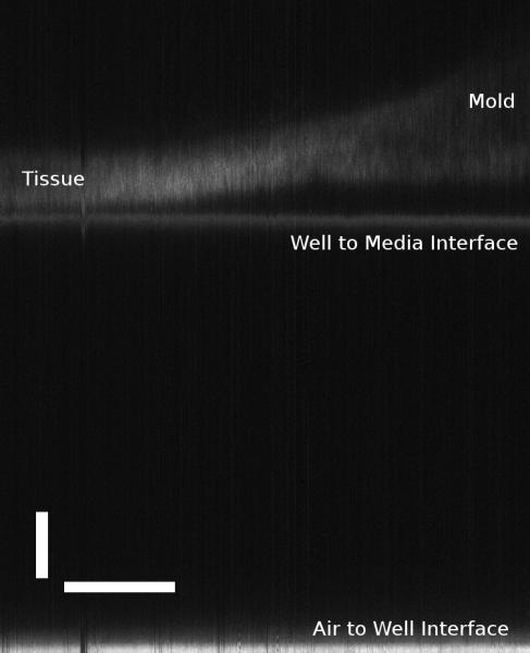
Confocal B-mode scan of a tissue sheet with mold using the confocal device. Horizontal scale bar is 1mm, and the vertical scale bar is 100μm.

Figure 6.

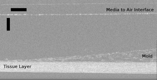
B-mode scan of a tissue sheet with mold using the OCT device. Horizontal scale bar is 200μm, and the vertical scale bar is 250μm.

The segmentation algorithm for the confocal scanner can be used on multiple B-mode scans to create a thickness map of large tissue sheets. Figure 7 shows the mechanically disturbed section of tissue sheet imaged over an area of approximately 68mm². Figure 7a is a thickness map obtained over the entire area using the segmentation algorithm. Thicker areas appear brighter in the map, with a maximum value in this case computed to be 189μm. Most of the tissue in this area appears to be approximately 100μm thick. For comparison, the thickness map of the same area is shown in Figure 7b taken by the OCT device.

Figure 7.

Side by side comparison of both modalities showing mechanically disturbed tissue. In both images, “A” is an external mark on the bottom of the well created by a fiber-tip pen. Hole “B” and slice “C” were created with a tip of a scalpel. Hole “D” was created with a 100μL pipette tip. (a) Confocal thickness map with calibrated intensity values (black: zero thickness to white: 189μm). Scale bar is 1.5mm. (b) Scaled thickness map of the same area scanned by OCT. Horizontal and vertical scale bars are each 1mm

A close-up of the scan taken of the punched hole (feature D in Figure 7) is shown in Figure 8 covering a total area of 0.403mm². A microscope image was taken of this same hole for comparison and shown in Figure 9. It can be seen that the darkest areas in Figure 8 coincide with the area where the pipette tip completely penetrated the tissue (no cells visible in Figure 9). The surrounding tissue appears to be approximately 100μm in thickness. Large thickness variation exists within this small area of tissue, most likely due to the manipulation of the tissue when pressed down by the pipette tip.

Figure 8.

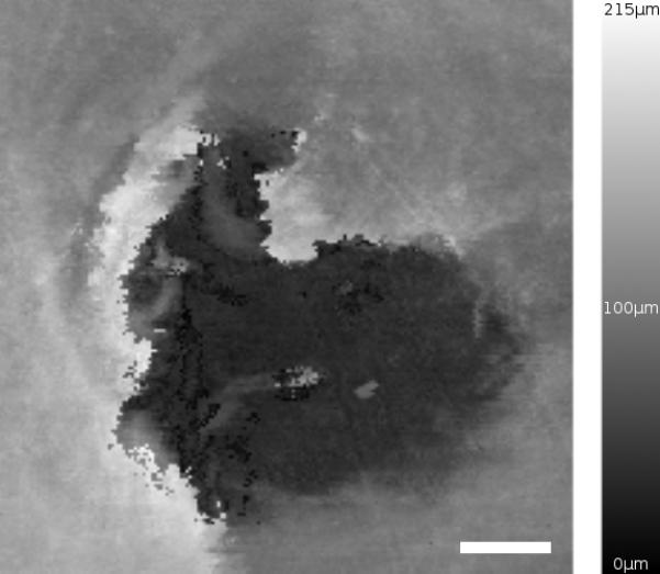
Confocal thickness map created by a high-resolution scan of area D in Figure 6. Scale bar is 100μm.

Figure 9.

Conventional brightfield microscope image of the area scanned in Figure 8. The image was taken on an inverted microscope and mirrored along the Y-axis for comparison to the confocal thickness map.

DISCUSSION

In this study, we presented an automated method to determine thickness and density of large tissue sheets based on a confocal scanner and an OCT scanner. In both imaging modalities, the signal is generated by refractive index changes, either by large-scale changes at interfaces or by subresolution changes commonly called scattering. Absorption can also cause contrast. In tissue, light is primarily scattered by collagen, and scattered light intensity may turn out to be related to collagen matrix expression of the cells. Experiments performed with the confocal scanner match observations found in Monte Carlo simulations.¹⁸ It can be seen that peaks caused by changes in refractive index are exhibited as sharper peaks, while peaks resulting from scattering regions appear broader. At interfaces, reflected intensity depends on the degree of refractive index change. Consequently, peak B is lower than Peak A in Figure 3, since the change in refractive index from the well to the tissue is only about 0.1, while the change from the air to the well is 0.47. When examining the measured FWHM of the imaging device, it becomes evident in Figures 2 and 3 that the FWHM of the peaks are broader than those obtained with OCT. The source of image blur is different in both instruments. Since axial pixel size of the OCT device is 3.1μm, it is difficult to accurately determine a more accurate FWHM of the peaks. For example, in Figure 2b, the FWHM of peak A appears to be 6.2μm, although the true FWHM may lie anywhere between 6.2μm and 18.6 μm due to limitations of pixel discretization of the device and partial-volume effects. In addition, the FWHM of peak B which was determined to be 18.6μm, a value closer to that of the confocal scanner of 24.45μm. Clearly, the predominant factor that limits resolution in the confocal scanner is Gaussian blur, while the limiting factor in the spectral radar OCT device is the source bandwith and the optical path difference between sample and reference beams.

Following confocal theory,¹⁹ the 3 dB separation distance of two focal planes, d_Z(3dB), is related to the refractive index n, the pinhole size a, the wavelength λ, and the objective magnification M through Equation 2:

$$d_Z\left(3dB\right)=\frac{7.4\cdot n\cdot a^2}{\lambda \cdot M^2}$$ (2)

Applying Equation 2 to our system, we found d_z to be 0.73μm from which the standard deviation σ of the Gaussian point-spread function can be calculated as 0.87μm. From this value, a theoretical FWHM of 2.1μm follows, a value markedly lower than the FWHM of the peaks found in Figure 3 (26.1μm for peak A and 13.4μm for peak B). For the OCT, the axial optical resolution is defined as ²⁰

$${\Delta }_z=\frac{2\ln 2}{\pi n}\cdot \frac{{\lambda }^2}{\Delta \lambda }$$ (3)

where Δz is the theoretical FWHM of the Gaussian point-spread function and Δλ is the FWHM of the bandwidth of the superluminescent laser diode. For our OCT system, Δz=3.8μm based on technical specifications, although the mirror scan yielded a FWHM of 6.2μm. Clearly, the main factor that limits the usability of the confocal scanner is the Gaussian blur introduced by several factors: the 50μm pinhole aperture that is dictated by the multimode fiber used in our prototype, possible underfilling of the objective, and our use of an objective that provided a long working distance at the expense of numerical aperture. A setup based on a very small single-mode fiber has been accomplished by a different research group,²¹ and design of future prototypes will take this concept into account, since a smaller pinhole should greatly improve the axial resolution. In a similar fashion, multiple factors play a role in determining the point-spread function of the OCT. In addition to the bandwidth of the light source (Equation 3), the point-spread function depends on the optical path difference between reference and sample path, and similar to the confocal scanner, the point-spread function that was actually measured was broader than expected from theory. Since a smaller FWHM of the point-spread function may be expected from theory, we cannot exclude the influence of manufacturing tolerances.

One additional possible solution to reduce the width of the point-spread function would be software deconvolution. If tissue thickness is the main parameter of interest, the empirical adjustment of the segmentation threshold would provide accurate thickness values. This notion is further corroborated by the comparable accuracy and precision of the thickness measurements in the OCT and confocal scanners. In the case of the confocal scanner, an excellent match with OCT-based thickness was observed in spite of the poorer point-spread function. However, both devices show a systematic deviation from caliper measurements in silicone samples of known thickness (Figure 4). We assume that the pressure exerted on the silicone samples by a micrometer-type caliper may compress the samples and cause this type of deviation - more compression in thicker samples. This consideration raises the question of precision. Clearly, mechanical measurements cannot provide precise measurements of sheet thickness, even if sample contamination is not taken into account. An experiment with repeated thickness measurement of tissue thickness after sample repositioning provided a standard deviation of 7.1μm in a 260μm sample, corresponding to a coefficient of variation of 2.7%. Considering the point-spread function of the confocal scanner, precision is not a major factor that influences the usability of the confocal scanner. Precision is also determined by the thresholding algorithm, particularly by the arbitrarily chosen factor a in Equation 1. Clearly, any Gaussian blur, whether caused by the optical system or by image processing, reduces the measured thickness with increasing a. While we consider a change of apparent tissue thickness of 0.5 pixels per percent-point change of a (this corresponds to roughly 3μm thickness change - about 1.2% of the thickness of a 260μm sheet - when a is changed from 50% to 60%) to be sufficiently reliable, two avenues can be tried to further reduce this potential source of error. First, a can be calibrated using samples of known thickness, such as the silicone sheets. Second, other edge-detection methods can be experimented with, such as application of the LoG (Laplacian-of-Gauss) operator. However, since the main limiting factor of the confocal scanner is the axial optical resolution, the improvement of the optical system should remain the primary focus.

While the thickness measurement by the automated segmentation algorithm can be considered reliable for normal tissue layers, the measured thickness of disturbed tissue or non-tissue features (such as mold) is uncertain. Some of the segmentation parameters have been empirically chosen and warrant a more thorough analysis with a larger sample set. Modifications of the segmentation algorithm would not change the principle of the actual confocal scanner. Both the coverslip thickness and the tissue thickness match the expected values and the values determined with OCT within few percent. Major deviations in the thickness measurements were observed in the mold scans. This is most likely due to the lack of differentiation of the mold and tissue caused by the filter step in the segmentation process. However, we included the mold scans for illustration purposes, as any mold accumulated on the tissue would invalidate the practical application of the tissue anyway. Therefore, determining the true thickness of the mold is irrelevant in this context.

A side by side comparison of the mechanically disturbed tissue images shown in Figure 7 illustrates the usefulness of the thickness map. It can be seen in the confocal image (Figure 7a) that there are thickness variations over the surface area of the tissue sheet. The thickness map generated by the confocal scanner is calibrated linearly over the thickness scale. Thickness variations are also visible in the OCT image (Figure 7b) but cannot easily be quantified because the OCT image was acquired with several scans, and the scans assembled manually to form the image in Figure 7b. Consequently, background intensity variations become visible that would adversely affect the estimated homogeneity of the tissue thickness. The source of these variations in a closed-source off-the-shelf OCT system remains unclear, and the observed intensity variations prohibit us from making a reliable comparison about thickness differences over the large scale. However, these considerations are limited to the specific OCT device that was used in this study. It is not unusual that details of the data collection and image formation software of off-the-shelf devices are not known, often being considered as trade secrets. A custom-built device, comparable to our custom confocal scanner, would not have any of these limitations, and a similar degree of automation would be possible. This notion can be taken further by custom-designing the optics at the end of the OCT sample arm. In fact, a more suitable sample scanning lens can be used to improve the lateral resolution of the device, as improving the bandwidth of the source would improve the axial resolution. However, the depth of focus is inversely related to the lateral resolution, and the limiting factor is the thickness of the flask bottom.

The ability of the confocal scanner to provide a wide range of lateral pixel sizes is illustrated further in Figure 8 which was taken at approximately 30 times higher resolution in each direction that Figure 7a. Such a scan would take 100 times longer over the same area than the low-resolution scan. On the other hand, the high-resolution scan compares well to the microscope brightfield image (Figure 9), where similarities in the hole shape can clearly be seen. The time factor could give rise to two scan modes: One initial scan at a low resolution, followed by high-resolution spot scans wherever thickness variations or other potential defects have been identified by software. Further software image processing is possible. One example is illustrated in Figure 10. A threshold of 125 μm has been applied, creating dark areas wherever tissue thickness falls below 125μm. This could be useful in quality control to determine where large areas of the tissue have not reached matured thickness. Similarly, the analysis of thickness variation could reveal inhomogeneously grown sheets.

Figure 10.

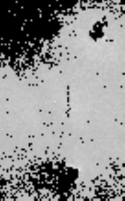
Confocal image showing mechanically disturbed tissue with thresholding at 125μm. Black regions indicate tissue sections with a thickness below 125 μm. This processed image is provided to demonstrate the ability of the confocal scanner to automatically identify inhomogeneous or thin tissue regions.

A comparison of the OCT and confocal scanners reveals advantages and disadvantages in both systems. Compared to OCT, a higher signal-to-noise ratio was observed in single (non-averaged) scans. Voxel size was smaller in the confocal scanner, leading to a potentially higher spatial resolution. In this specific case, confocal spatial resolution was primarily confounded by the large FWHM. Furthermore, the OCT scanner was dramatically faster than the confocal scanner. The z-stage used in the confocal scanner prototype allowed us to perform one A-mode scan in 9 seconds, while the OCT scanner provided one B-mode scan in 0.25 seconds. Acquisition and averaging of ten OCT B-mode scans for improved SNR was still faster than one confocal A-mode scan. Clearly, the two most important areas for improvement of the confocal scanner are the axial translation mechanism (faster fine-positioning in the axial direction by using, for example, a piezoelectric positioner) and the fiberoptic system, where an optimum pinhole size needs to be found.

In conclusion, we found that both OCT and confocal scattered-light imaging in combination with suitable image processing are viable methods to determine the thickness of tissue-engineered sheets. Our experience with the off-the-shelf OCT device showed us that a custom design allows for more complete system integration and full automation. This study also demonstrated that a confocal scattered-light scanner is feasible, but additional improvements are required to convert our prototype into a device that can be used in routine quality control for engineered tissue sheets. In sheets that are typical for this application, that is, sheets between 100μm and 300μm thickness, both the OCT and the confocal principle can be used. Provided that the FWHM of the confocal scanner can be improved, its smaller voxel size makes confocal imaging more suitable than OCT for thin tissue sheets, while thicker sheets cannot be imaged with the confocal scanner. Both imaging techniques, in combination with suitable image processing, promise to become useful enabling technologies for automated quality control in tissue engineering.

References

- 1.Fodor WL. Tissue engineering and cell based therapies, from the bench to the clinic: the potential to replace, repair and regenerate. Reprod.Biol.Endocrinol. 2003;1:102. doi: 10.1186/1477-7827-1-102. [DOI] [PMC free article] [PubMed] [Google Scholar]
- 2.Griffith LG, Naughton G. Tissue engineering - Current challenges and expanding opportunities. Science. 2002;295:1009. doi: 10.1126/science.1069210. + [DOI] [PubMed] [Google Scholar]
- 3.Yang J, Yamato M, Nishida K, Ohki T, Kanzaki M, Sekine H, Shimizu T, Okano T. Cell delivery in regenerative medicine: The cell sheet engineering approach. Journal of Controlled Release. 2006;116:193–203. doi: 10.1016/j.jconrel.2006.06.022. [DOI] [PubMed] [Google Scholar]
- 4.Yang J, Yamato M, Nishida K, Hayashida Y, Shimizu T, Kikuchi A, Tano Y, Okano T. Corneal epithelial stem cell delivery using cell sheet engineering: Not lost in transplantation. Journal of Drug Targeting. 2006;14:471–482. doi: 10.1080/10611860600847997. [DOI] [PubMed] [Google Scholar]
- 5.Lai JY, Chen KH, Hsiue GH. Tissue-engineered human corneal endothelial cell sheet transplantation in a rabbit model using functional biomaterials. Transplantation. 2007;84:1222–1232. doi: 10.1097/01.tp.0000287336.09848.39. [DOI] [PubMed] [Google Scholar]
- 6.Vesely I. Heart valve tissue engineering. Circulation Research. 2005;97:743–755. doi: 10.1161/01.RES.0000185326.04010.9f. [DOI] [PubMed] [Google Scholar]
- 7.Neuenschwander S, Hoerstrup SP. Heart valve tissue engineering. Transplant Immunology. 2004;12:359–365. doi: 10.1016/j.trim.2003.12.010. [DOI] [PubMed] [Google Scholar]
- 8.Masuda S, Shimizu T, Yamato M, Okano T. Cell sheet engineering for heart tissue repair. Advanced Drug Delivery Reviews. 2008;60:277–285. doi: 10.1016/j.addr.2007.08.031. [DOI] [PubMed] [Google Scholar]
- 9.Shimizu T, Yamato M, Kikuchi A, Okano T. Cell sheet engineering for myocardial tissue reconstruction. Biomaterials. 2003;24:2309–2316. doi: 10.1016/s0142-9612(03)00110-8. [DOI] [PubMed] [Google Scholar]
- 10.L’Heureux N, McAllister TN, de la Fuente LM. Tissue-engineered blood vessel for adult arterial revascularization. New England Journal of Medicine. 2007;357:1451–1453. doi: 10.1056/NEJMc071536. [DOI] [PubMed] [Google Scholar]
- 11.L’Heureux N, Dusserre N, Marini A, Garrido S, de la Fuente L, McAllister T. Technology Insight: the evolution of tissue-engineered vascular grafts - from research to clinical practice. Nature Clinical Practice Cardiovascular Medicine. 2007;4:389–395. doi: 10.1038/ncpcardio0930. [DOI] [PubMed] [Google Scholar]
- 12.Welzel J. Optical coherence tomography in dermatology: a review. Skin Research and Technology. 2001;7:1–9. doi: 10.1034/j.1600-0846.2001.007001001.x. [DOI] [PubMed] [Google Scholar]
- 13.Farkas DL, Becker D. Applications of spectral imaging: Detection and analysis of human melanoma and its precursors. Pigment Cell Research. 2001;14:2–8. doi: 10.1034/j.1600-0749.2001.140102.x. [DOI] [PubMed] [Google Scholar]
- 14.Ripandelli G, Coppe AM, Capaldo A, Stirpe M. Optical coherence tomography. Semin Ophthalmol. 1998;13:199–202. doi: 10.3109/08820539809056053. [DOI] [PubMed] [Google Scholar]
- 15.Hrynchak P, Simpson T. Optical coherence tomography: An introduction to the technique and its use. Optometry and Vision Science. 2000;77:347–356. doi: 10.1097/00006324-200007000-00009. [DOI] [PubMed] [Google Scholar]
- 16.Schaudig U. Optical coherence tomography. Ophthalmologe. 2001;98:26–34. doi: 10.1007/s003470170196. [DOI] [PubMed] [Google Scholar]
- 17.Fujimoto JG. Optical coherence tomography for ultrahigh resolution in vivo imaging. Nature Biotechnology. 2003;21:1361–1367. doi: 10.1038/nbt892. [DOI] [PubMed] [Google Scholar]
- 18.Dunn AK, Smithpeter C, Welch AJ, Richards-Kortum R. Sources of contrast in confocal reflectance imaging. Applied Optics. 1996;35:3441–3446. doi: 10.1364/AO.35.003441. [DOI] [PubMed] [Google Scholar]
- 19.Corle TR, Kino GS. Confocal scanning optical microscopy and related imaging systems. Academic Press; San Diego: 1996. [Google Scholar]
- 20.Leitgeb RA, Drexler W, Unterhuber A, Hermann B, Bajraszewski T, Le T, Stingl A, Fercher AF. Ultrahigh resolution Fourier domain optical coherence tomography. Optics Express. 2004;12:2156–2165. doi: 10.1364/opex.12.002156. [DOI] [PubMed] [Google Scholar]
- 21.Ilev I, Waynant R, Gannot I, Gandjbakhche A. Simple fiber-optic confocal microscopy with nanoscale depth resolution beyond the diffraction barrier. Review of Scientific Instruments. 2007;78:093703. doi: 10.1063/1.2777173. [DOI] [PubMed] [Google Scholar]
- 22.L’Heureux N, Pâquet S, Labbé R, Germain L, Auger FA. A completely biological tissue-engineered human blood vessel. FASEB J. 1998;12:47–56. doi: 10.1096/fasebj.12.1.47. [DOI] [PubMed] [Google Scholar]