Computer-aided diagnosis of pulmonary nodules on CT scans: Segmentation and classification using 3D active contours

Abstract

We are developing a computer-aided diagnosis (CAD) system to classify malignant and benign lung nodules found on CT scans. A fully automated system was designed to segment the nodule from its surrounding structured background in a local volume of interest (VOI) and to extract image features for classification. Image segmentation was performed with a three-dimensional (3D) active contour (AC) method. A data set of 96 lung nodules (44 malignant, 52 benign) from 58 patients was used in this study. The 3D AC model is based on two-dimensional AC with the addition of three new energy components to take advantage of 3D information: (1) 3D gradient, which guides the active contour to seek the object surface, (2) 3D curvature, which imposes a smoothness constraint in the z direction, and (3) mask energy, which penalizes contours that grow beyond the pleura or thoracic wall. The search for the best energy weights in the 3D AC model was guided by a simplex optimization method. Morphological and gray-level features were extracted from the segmented nodule. The rubber band straightening transform (RBST) was applied to the shell of voxels surrounding the nodule. Texture features based on run-length statistics were extracted from the RBST image. A linear discriminant analysis classifier with stepwise feature selection was designed using a second simplex optimization to select the most effective features. Leave-one-case-out resampling was used to train and test the CAD system. The system achieved a test area under the receiver operating characteristic curve (A_z) of 0.83±0.04. Our preliminary results indicate that use of the 3D AC model and the 3D texture features surrounding the nodule is a promising approach to the segmentation and classification of lung nodules with CAD. The segmentation performance of the 3D AC model trained with our data set was evaluated with 23 nodules available in the Lung Image Database Consortium (LIDC). The lung nodule volumes segmented by the 3D AC model for best classification were generally larger than those outlined by the LIDC radiologists using visual judgment of nodule boundaries.

I. INTRODUCTION

Lung cancer is the leading cause of cancer death for both men and women in the United States, accounting for 28% of all cancer deaths, or an estimated 163 510 lives in 2005. More people die from lung cancer than from colon, breast, and prostate cancers combined. While the five-year survival rate for lung cancers is only 15%, if detected and treated at its earliest stage (stage I), the five-year survival rate increases to 47%.¹ Unfortunately, most patients present clinically with advanced stage disease. The lack of a generally accepted screening test to reduce lung cancer mortality contributes to the poor prognosis of lung cancer. Furthermore, existing diagnostic tests to evaluate lung nodules are insufficient, with many lung nodules classified as indeterminate for malignancy. For this reason, approximately half of the indeterminate lung nodules resected at surgery are benign.² Reducing the number of biopsies for benign nodules will reduce health care costs and patient morbidity.

The Early Lung Cancer Action Project (ELCAP) was initiated in 1992 to assess the usefulness of annual low dose computed-tomography (CT) screening for lung cancer in a high-risk population.³ Initial findings from the baseline screening of 1000 patients indicated that low dose CT can detect four times the number of malignant lung nodules and six times more stage I malignant nodules than chest radiography. These results have been confirmed by several groups of investigators.^4–10 These data suggested a strong potential for improving the likelihood of detecting lung cancer at an earlier and potentially more curable stage with CT.¹³ The ongoing National Lung Screening Trial funded by the National Cancer Institute is the first multicenter, randomized controlled trial to evaluate the effectiveness of helical CT versus chest radiography for lung cancer screening.

Although CT may be more sensitive than chest radiography for the detection of lung cancer, potential impediments to the use of helical CT for lung cancer screening exist. For example, the chance of false negative detection due to the large volume of images in each multidetector CT examination is not negligible, the management of the large number of benign nodules or false-positive results that are detected may limit the cost-effectiveness of screening CT, and the follow up of nodules found on CT with serial CT examinations increases radiation exposure to the population.¹⁰ One solution to address some of these issues may be computer-aided diagnosis (CAD), which has been shown to increase the sensitivity of breast cancer detection on mammography screening in clinical practice.¹¹ Computer-aided detection may reduce false negative detections, while computer-aided diagnosis (characterization) may increase the discrimination between malignant and benign nodules.

CAD systems typically involve the steps of segmentation, feature extraction, and classification. Various methods used in medical image segmentation such as thresholding,¹² region growing,^13,14 and level sets^15,16 have been evaluated. Segmentation of organs or other structures where the general shape is known has been performed with atlas-based segmentation methods.¹⁷ While these methods may be effective for specific types of lesions and images, pulmonary nodules present a challenging problem due to their variability in shape and anatomic connection to neighboring pulmonary structures, such as blood vessels and the pleural surface.

Previous CAD development for CT focused mainly on automated detection.^12,18–25 Recently there has been more work on the classification of malignant and benign nodules. McNitt-Gray et al. obtained 90.3% correct classification accuracy between 14 malignant and 17 benign cases.²⁶ Shah et al. achieved A_z values between 0.68 and 0.92 with 48 malignant and 33 benign nodules, using four different types of classifiers in a leave-one-out method. Features were extracted from contours manually drawn on a single representative slice of each nodule.²⁷ Armato et al. used an automated detection scheme, then manually separated nodules from non-nodules for the classification step. They achieved an A_z value of 0.79 using features such as radius of sphere of equivalent volume, minimum and maximum compactness, gray-level threshold, effective diameter, and location along the z axis.²⁸ Kawata et al. used surface curvatures and ridge lines as features for description of 62 cases including 47 malignant and 15 benign nodules, showing good evidence of separation between malignant and benign classes in feature maps; no A_z value was reported.²⁹ Li et al. reported an A_z of 0.937 for distinction between 61 malignant and 183 benign nodules in a leave-one-out testing method, and an A_z of 0.831 for a randomly selected subset consisting of 28 primary lung cancers and 28 benign nodules.³⁰ Features used included diameter, contrast of segmented nodule, and those extracted from gray-level histograms of pixels inside and outside the segmented nodule. Aoyama et al. reported an A_z of 0.846 for classifying 76 primary lung cancers and 413 benign nodules using multiple slices(10 mm collimation and 10 mm reconstruction interval), which was a statistically significant improvement over 0.828 when only using single slices.³¹ Suzuki et al. obtained an A_z of 0.882 by use of a massive training artificial neural network (MTANN) on a data set of 76 malignant and 413 benign nodules.³²

We are developing an automated system for classification of malignant and benign nodules extracted from CT volumes. Nodules were segmented from the image background using a three-dimensional (3D) active contour (AC) method. Malignant and benign nodules were differentiated using morphological and texture characteristics. The weights for the energy terms in the AC model were optimized using the classification accuracy as a figure-of-merit. Our initial experience in nodule classification is reported in this paper. For comparison, we also analyzed the classification performance using radiologists’ subjective estimation of likelihood of malignancy and a classifier designed with feature descriptors provided by radiologists. The segmentation performance of the 3D AC model trained with our method was evaluated with 23 nodules available from the Lung Image Database Consortium (LIDC).

II. METHODS AND MATERIALS

A. Data sets

1. Clinical data set

We analyzed 96 lung nodules (44 malignant and 52 benign) from 58 patients. All cases were collected with Institutional Review Board approval. Of the 44 malignant nodules, 25 were biopsy-proven to be malignant, and 19 nodules were determined to be malignant either through positive PET scans or known metastatic nodules from confirmed cancers in other body parts. Of the 44 malignant nodules, 15 were primary cancers and 29 were metastases. Of the 52 benign nodules, 10 were biopsy-proven and 42 were determined to be benign by two-year follow-up stability on CT. Of the 96 nodules, 20 (21%) were juxta-pleural and 12 (12.5%) were juxta-vascular as indicated by expert radiologists.

Each CT image was 512 × 512 pixels. The CT scans were acquired with either GE Lightspeed CT/I (single-slice helical), QX/I (4 slice), Ultra (8 slice), or LightSpeed Plus (8 slice) scanners, using imaging techniques of 120 kVp, 80–400 mA, and reconstructed slice interval of 1.25–5 mm. Linear interpolation was performed in the z direction to obtain isotropic voxels before initial contour generation and segmentation to facilitate the implementation of the 3D segmentation and feature extraction operations in the CAD system. The interpolation does not recover the reduced spatial resolution in the z direction.

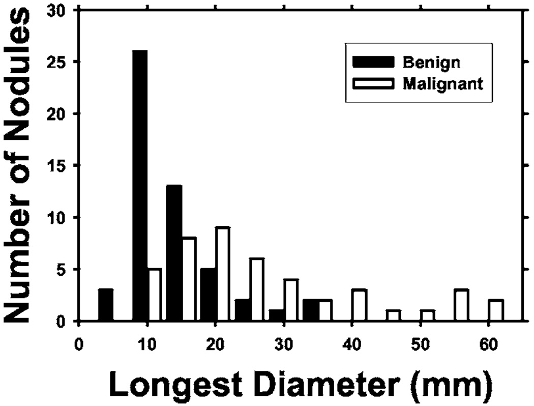
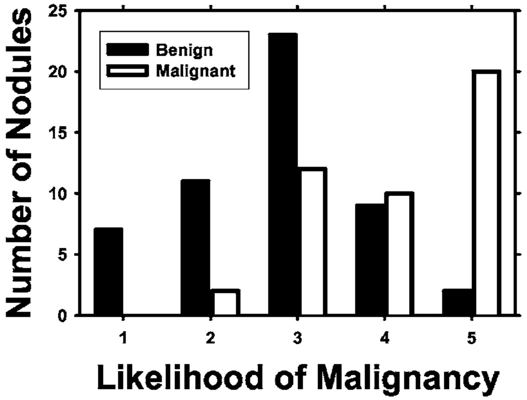
A user interface was developed for displaying the CT images and recording nodule locations and ratings provided by radiologists. Two radiologists were trained in using the software and giving ratings for the data set. Each case was read by one of these experienced thoracic radiologists who marked volumes of interest (VOIs) that contained lung nodules. For each nodule, a confidence rating of the likelihood of malignancy on a 5-point scale was provided, 5 being the most likely to be malignant. Electronic rulers were used to measure the longest diameter of each nodule as seen on axial slices. The radiologists also recorded various feature descriptors for each nodule, such as conspicuity, edge (smooth, lobulated, or spiculated/irregular), and the presence of calcification. Each radiologist read approximately half of the cases. The distribution of the longest diameters of the 96 nodules is shown in Fig. 1. The longest diameter ranged from 3.9 to 59.8 mm, with a median of 13.3 mm and mean of 17.3 mm. Figure 2 shows the distribution of the malignancy ratings of the nodules by the radiologists. The malignancy ratings for benign and malignant nodules overlap substantially, confirming that visual characterization of the nodules on CT images is not a simple task.

Fig. 1.

Distribution of the longest diameters of the lung nodules in the data set, as measured by experienced thoracic radiologists on the axial slices of the CT examinations.

Fig. 2.

Confidence ratings for the likelihood of a nodule being malignant (1 = most likely benign, 5 = most likely malignant) by experienced thoracic radiologists.

2. LIDC data set

The 23 nodules available to-date from the data set provided by the LIDC³³ were used for testing our 3D AC model. The LIDC database is intended to be a common data set available to all researchers for development of CAD systems and for comparison of their performance. The data set includes “gold standard” segmentation of each nodule by six expert chest radiologists. Each radiologist performed one manual and two semi-automatic markings of each nodule, resulting in a total of 18 boundaries for each. The 18 boundaries were used to generate a probability map (pmap), which was scaled to a range of 0 to 1000. A boundary of the nodule at a pmap threshold of 500, for example, is a contour that encloses all the voxels with values greater than or equal to 500, which means that those voxels were considered to be part of the nodule by more than 50% of the 18 “gold standard” segmentations. More information about the database can be found on the LIDC website, where the images are also free for download: (http://imaging.cancer.gov/reportsandpublications/reportsandpresentations/firstdataset).

B. Initial contour determination

Our nodule segmentation method has two steps: estimation of an initial boundary by k-means clustering and refinement of the boundary with a 3D active contour model. The VOI determined by the radiologist may contain other pulmonary structures in addition to the nodule, such as blood vessels or voxels that are outside the lung region (chest wall or mediastinum). A lung region mask determined by our automated nodule detection system described in the literature¹⁸ is first applied to the VOI to exclude the voxels belonging to the chest wall or the pleura from further processing. Then a 3D weighted k-means clustering method³⁴ based on CT values is used for initial segmentation of the nodule from the other structures in the VOI. The VOI is assumed to contain two classes: the lung nodule (including other tissue but excluding the chest wall) and the background. Clustering is performed iteratively until the cluster centers of the classes stabilize as described elsewhere.³⁴ The voxels grouped into the nonbackground class may or may not be connected. A 26-connectivity criterion is used to determine the various connected objects in the 3D space and the largest one closest to the center is chosen as the nodule. We can make this assumption because of the a priori knowledge that the VOI contains a nodule and that this study is focused on classification, not on detection (determining whether objects are true nodules).

The lung nodule segmented by clustering may be attached to blood vessels or other structures. Once this main object is identified in the VOI, 3D morphological opening with a spherical structuring element is applied to the object to trim off some connected vessels or structures. The structuring element is chosen to be spherical in this application because nodules tend to be spherical in shape, while non-nodule objects such as blood vessels tend to be cylindrical. For each slice intersecting the object in the VOI, the radius of an equivalent circle with the same area was found. The radius of the structuring element was chosen experimentally as the average of the radii subtracted by 1. Equivalent radii of cross sections are used because the partial volume effect makes some objects more cylindrical than they truly are, resulting in structuring elements that are too large if volumes are used in the calculation. After morphological opening, the boundary of the resulting object is used as the initial contour for the active contour segmentation.

C. 3D active contour segmentation

1. The active contour model

Deformable contour models, particularly the AC model introduced in the seminal paper by Kass et al.,³⁵ are well-known tools for image segmentation. Active contours are energy-minimizing splines guided by various forces, or energies. The internal energies impose constraints on the contour itself, while external energies push the contour toward salient image features such as lines and edges. The contour is represented as a vector v(s) = (x(s), y(s)), where s is the parameter arclength. The energy functional is defined as

$$E_{\text{snake}}^{*}={\displaystyle {\int }_0^1{E}_{\text{snake}}(\upsilon (s))\mathit{\text{ds}}.}$$ (1)

The $E_{\text{snake}}^{*}$ energy contains the various energy components that will be discussed later along with the energies we contribute. Segmentation of the object using the AC is thus achieved by minimizing $E_{\text{snake}}^{*}$.

2. Parametric implementation of continuous splines

Using variational calculus or dynamic programming to minimize the total energy of the parametric representation of a continuous contour can result in instability and a tendency for points to bunch up together.³⁶ Instead of a continuous contour representation, the AC optimization algorithm in this study represents the contour by a set of vertices and uses a greedy algorithm to find the solution. The neighborhood for vertex v(c), c = {1,2,…,N}, is examined at each iteration, where N is the total number of polygon vertices. The vertex is then moved to the pixel with the minimum contour energy E_min(v(c)). The process repeats until the number of vertices that moves is below a threshold. The final contour is obtained by minimizing the cost function:

$$\begin{array}{cc}{E}_{\text{total}}=\hfill & \underset{E(c)}{\text{min}}{\displaystyle \sum _{c=1}^N[w_{\text{hom}}{E}_{\text{hom}}(c)+w_{\text{cont}}{E}_{\text{cont}}(c)+w_{\text{curv}}{E}_{\text{curv}}(c)}\hfill \\ \hfill & +w_{3\text{Dcurv}}{E}_{3\text{Dcurv}}(c)+w_{\text{grad}}{E}_{\text{grad}}(c)\hfill \\ \hfill & +w_{3\text{Dgrad}}{E}_{3\text{Dgrad}}(c)+w_{\text{bal}}{E}_{\text{bal}}(c)+w_{\text{mask}}{E}_{\text{mask}}(c)],\hfill \end{array}$$ (2)

where E(c) is the energy at a pixel in the neighborhood of vertex v(c) = (x(c), y(c)), c∈{1,2,…,N}. In this energy functional, the internal energies include homogeneity (hom), continuity (cont), curvature (curv), 3D curvature (3Dcurv), and the external energies include gradient (grad), 3D gradient (3Dgrad), balloon (bal), and mask (mask). The weight w_j is a parameter assigned to each energy j, where j represents one of the eight energies: hom, cont, curv, 3Dcurv, grad, 3D grad, bal, and mask.

3. Two-dimensional energies

In this preliminary study, the energy terms other than 3D curvature and 3D gradient are calculated on the x-y planes of the CT slices intersecting the nodule. The vertices on each slice move in the x-y plane during the iteration. The continuity of the segmented nodule area between different slices is constrained by the 3D curvature and the 3D gradient terms which provide the 3D information in the current model.

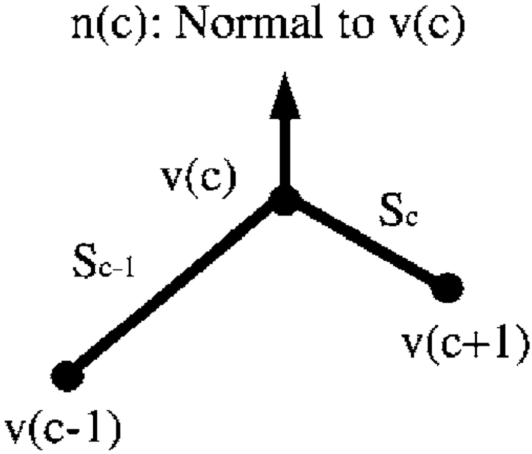
A brief description of the two-dimensional (2D) energy components is given here. Details can be found elsewhere in the literature.^36–38 Homogeneity energy³⁷ is a measure of how similar the pixel intensities inside the contour are. The contour divides each region-of-interest (ROI) into two regions: the area enclosed by the contour and the background excluding the chest wall. We seek to minimize the intensity variation within each region while maximizing the difference of the mean intensities between the two regions. The homogeneity energy is therefore calculated as the ratio of the within-regions sum of squares to the between-region sum of squares of the gray levels in the two regions. The continuity energy maintains regular spacing between the vertices of the contour. If the points could move in the neighborhood without this constraint, then they might move toward one another, leading to the ultimate collapse of the contour. The continuity energy is calculated as the deviation of the length of line segment between two vertices from the average line segment length over all vertices. The curvature energy smoothes the contour by discouraging small angles at vertices. There are many ways of estimating curvature, as investigated by Williams and Shah.³⁶ In our implementation, the second-order derivative along the contour is approximated by finite differences. If v(c) is a point on the contour as depicted in Fig. 3, then the second-order derivative at v(c) is |v(c−1)−2v(c) +v(c+1)|, which is used as the curvature energy. If the angle where two segments meet at a vertex is small, then this term will be large; conversely, when the angle is large, a low energy value results.

Fig. 3.

The vertices of the polygon and positions used in the active contour model.

The balloon energy prevents the contour from collapsing onto itself, which is a well-known phenomenon for AC segmentation.³⁹ The normal direction n(c) to the contour is defined as the average of the normals to the two sides of the polygon that meet at vertex v(c). Let v′(c) be the new position where vertex v(c) moves to in the neighborhood. The balloon energy can then be calculated as the cosine of the angle between n(c) and v′ (c)−v(c). The weight w_bal determines whether the contour expands in the normal direction or the direction opposite to the normal. If the weight is negative, then a point moving farther along the normal direction will lower the energy, thus expanding the contour.

The gradient energy attracts the contour to object edges. To calculate the gradient magnitude, the image is first smoothed with a low-pass filter, chosen experimentally to be a Gaussian filter, F(x, y) = e^{−(x2+y2)/σ2}, with σ = 300 µm. The partial derivatives are found in the vertical and horizontal direction, and the magnitude of the resulting vector is computed. The energy is defined as the negative of the gradient magnitude, so object edges with high gradient magnitudes will attract the contour. For image I(x, y), the gradient energy is calculated as

$$E_{3\text{Dgrad}}(c)=-{|\overrightarrow{\nabla }(\mathrm{I}{(x,y)}^{**}F(x,y))|}^2,$$ (3)

where ** denotes 2D convolution, and ∇⃗ is the partial derivative gradient operator.

4. New energies

a. 3D gradient

The 3D gradient energy is defined in a similar way to the 2D gradient energy. The 2D gradient magnitude image shows the edges of the object in the 2D image, but the 3D gradient magnitude image reveals the surface of the object, thus giving better shape information of the nodule. The 3D image containing the nodule is first smoothed with a 3D low-pass Gaussian filter:

$$F(x,y,z)=\frac{1}{{(2\mathrm{\pi })}^{3/2}\mathrm{\sigma }}\text{exp}\left[-\frac{1}{2}\frac{(x^2+y^2+z^2)}{{\mathrm{\sigma }}^2}\right].$$ (4)

The energy is calculated in a similar way to the 2D method:

$${\mathrm{E}}_{3\text{Dgrad}}(c)=-{|\overrightarrow{\nabla }(\mathrm{I}{(x,y,z)}^{**}F(x,y,z))|}^2.$$ (5)

b. 3D curvature

We introduced the 3D curvature energy to take advantage of the information in the z direction, which we found to improve segmentation results over 2D energies alone.⁴⁰ This energy is an extension of the curvature constraint idea in 2D, where the energy is calculated using the two nearest neighbor vertices. In 3D, the energy for each vertex is calculated with the nearest points on the contours above and below the current contour. With this energy, the 2D contour at a given slice will thus be constrained by the adjacent contours above and below. This prevents one contour from varying substantially from other contours and results in an overall smoothness in the z-direction.

To calculate this energy for vertex v_i(c) of the contour on the ith slice, the closest points to v_i(c) on the contours in the slices above and below i are determined. Let v_i+1(c_i+1) and v_i−1(c_i−1) denote the closest points to vertex c on slices (i+1) and (i−1), respectively. Since these points are defined to be lying on the contours, they may be on the lines between vertices and are not necessarily the vertices that move during deformation of other slices. Note that the index of the point on the contour of the (i+1)th and (i−1)th slices may not be the same as c and, in fact, they may not be vertices of the contours. As described earlier, we used two new indices with subscripts, c_i−1 and c_i+1, to denote that these are different indices on the respective contours. The 3D curvature energy is represented by an approximation to the second derivative of the contour in the z direction,

$$E_{3\text{Dcurv}}(c)=\left|{\mathbf{v}}_{i-1}(c_{i-1})-2{\mathbf{v}}_i(c)+{\mathbf{v}}_{i+1}(c_{i+1})\right|.$$ (6)

c. Mask energy

Nodules attached to the pleura (juxta-pleural nodules) present a challenge to segmentation. Both nodules and normal body tissues have a similar range of Hounsfield Units (HU). Region growing or thresholding methods will fail to segment nodules, because the pleura, chest wall, or mediastinum may be included in the contour. Gradient-based methods will not be able to detect the edge of the nodule either, as there is no well-defined boundary between nodule and normal tissues. Kostis⁴¹ proposed connecting the two points of highest curvature (where the boundary of the pleura meets that of the nodule) and estimating the curvature of the wall boundary. That method may not be sensitive enough to local concavities, due to anatomic or pathological variations.

We have designed a mask energy to meet this challenge. The mask energy is a function of the distance from a vertex on the AC contour of the nodule to the lung boundary. This is calculated for each vertex that moves beyond the lung boundary (in the pleura or thoracic wall) during each iteration of the energy-minimizing procedure. An accurate lung boundary is therefore required for determining the mask energy. We will describe in the following our methods for finding the initial lung boundary and the subsequent local refinement used to produce an accurate boundary.

The first step is to determine the boundary of the pleura. Because of different CT scanning parameters, the k-means clustering technique with CT voxel value as the feature is used to segment the lung regions from the thorax in each CT slice instead of a simple threshold. The extracted lung regions are represented by polygons marking the lung boundaries. This process provides the initial lung boundaries in the entire slice. More details on this process may be found in the literature.¹⁸

The initial lung boundaries are a general outline of the lungs, but they may not be sensitive enough to exactly delineate the boundary between a nodule and the pleural surface. If the estimated lung boundary is not close enough to the actual boundary, it may even trim off part of a juxtapleural nodule. To refine the boundary between a juxtapleural nodule and the pleural surface, we use k-means clustering³⁴ within each VOI to determine the mean and standard deviation of the voxel values considered to be background (lung regions). Any voxels originally considered part of the pleura, chest wall, or mediastinum that fall within 3 s.d. of this range will have their membership changed to be that of the lung region. The threshold of 3 s.d. was chosen experimentally based on the separation between the distributions of voxel values of the nodules and the lung regions in the training samples. As depicted in Fig. 4, an indentation was created as the refined boundary included more of the area originally considered chest wall into the lung region.

Fig. 4.

An example demonstrating the correction of lung segmentation from the pleural surface. From left to right: the initial pleural boundary, indentation created along the lung boundary after local refinement, and corrected lung boundary after indentation is filled.

An indentation detection¹⁸ technique is used to fill in that indentation. This method detects an indentation by means of distance ratios. For every pair of points P₁ and P₂ along the lung boundary, three distances are calculated. Distances d₁ and d₂ are distances between P₁ and P₂ measured by traveling along the boundary in the counterclockwise and clockwise directions, respectively. The third distance d_e is the Euclidean distance between P₁ and P₂. The ratio is calculated:

$$R_e=\frac{\text{min}(d_1,d_2)}{d_e}.$$ (7)

If the ratio is greater than a threshold, then an indentation is assumed, and it is filled by connecting the points P₁ and P₂ with a straight line. R_e was chosen to be 1.5 in our previous study.¹⁸ Figure 4 shows an example how the boundary improves as a result of this method.

This boundary marks where the lung region is. If a vertex of the nodule contour v(c) moves to a position v′(c) that falls outside of the lung region into the chest wall, the mask energy is calculated as

$$E_{\text{mask}}=|\mathbf{b}(c)-{\mathbf{v}}^{\prime }(c)|,$$ (8)

where b(c) is the point on the lung boundary closest to v(c). Instead of outright forbidding the nodule contour to grow into the chest wall, this energy allows for the fact that the lung boundary may not be completely accurate. The contour may grow into the chest wall, but it will be penalized the further away from the chest wall boundary it grows.

D. Feature extraction

Gurney⁴² has provided likelihood ratios for various characteristics that may be useful for discriminating malignant from benign nodules. Other features to discriminate malignant from benign nodules have been described by Erasmus.⁴³ We seek to quantify the characteristics of nodules by mathematical feature descriptors. The accuracy of the segmentation is important for extraction of some of the features. There is no single feature that can accurately determine whether a nodule is benign or malignant. For example, features such as the presence of calcification may be a strong indicator that a nodule is benign. However, it has been reported that 38%–63% of benign nodules are noncalcified,^43–45 and in the study by Swensen et al.,⁹ up to 96% benign nodules were noncalcified.

From the segmented nodule boundary, we extracted a number of morphological features including volume, surface area, perimeter, maximum diameter, and maximum and minimum CT value (HU) inside the nodule. We also extracted statistics from the gray-level intensities of voxels inside the nodule including the average, variance, skewness, and kurtosis of the gray-level histogram.

In addition to features that can be derived from the inside of the nodule, the tissue texture around the margin of the nodule is also important. The growth of malignant tumors tends to distort the surrounding tissue texture, while benign nodules tend to have smooth surfaces with more uniform texture around them. To derive these features from the texture around the nodule, the rubber band straightening transform (RBST) is first applied to planes of voxels surrounding the nodule. The run-length statistics (RLS) texture features are then extracted from the transformed images, as described in the following.

E. Rubber band straightening transform (RBST)

The RBST was introduced by Sahiner et al.⁴⁶ for analysis of the texture around mammographic masses on 2D images. The RBST image is obtained by traveling along the boundary of the nodule, transforming the band of pixels surrounding the nodule into a rectangular image. In this way, spicules that grow out radially from an object may be transformed as approximately straight lines in the y direction.

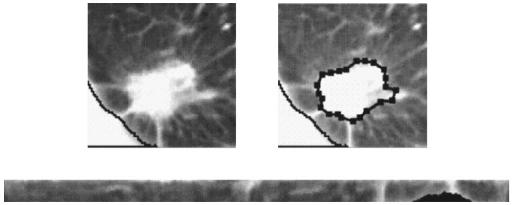
The RBST maps a closed path at an approximately constant distance from the nodule boundary of the original image to a row in the transformed image, as depicted in Fig. 5. The difference between the RBST and the transformation from Cartesian to polar coordinates is that the irregular or jagged lesion boundary will be transformed to a straight line in the horizontal direction, whereas in a Cartesian to polar transformation, only a circle of constant radius will be transformed to a horizontal straight line.

Fig. 5.

The rubber band straightening transform (RBST). Top Left: A ROI containing a nodule. Top Right: The active contour boundary from which the RBST image is extracted. Bottom: The RBST image that will be Sobel-filtered, from which run-length statistics may be extracted. The black area of the RBST image corresponds to the pixels where the chest wall is masked out.

With 3D CT scan data, the texture around the whole nodule needs to be extracted. We apply the RBST to the original CT slices to extract texture in the axial planes. To adequately sample the texture in all directions, we slice the nodule with two additional sets of planes: by considering the nodule as a globe, one set contains the longitude lines that run through the north and south poles (z direction in a CT scan), and the other through the east-west poles. In each set, four oblique planes (45° apart) slice evenly along the lines of longitude on the nodule surface. The RBST is applied to a band of voxels surrounding the nodule on each of the oblique planes. Each RBST image is then enhanced by Sobel filtering in both the horizontal and vertical directions. Texture features based on run-length statistics are extracted from the Sobel-filtered RBST images.

RLS texture features were introduced by Galloway⁴⁷ to analyze the number of runs of a gray level in an image. A run-length matrix p(i, j) stores information of the number of runs with pixels of gray-level i and run length j. In this study, the 4096 gray levels are binned into 128 levels before the run-length matrix is constructed to improve the statistics in the matrix. Galloway designed five RLS features extracted from p(i, j) to describe the gray level patterns in the image: Short Runs Emphasis (SRE), Long Runs Emphasis (LRE), Gray-Level Nonuniformity (GLN), Run Length Nonuniformity (RLN), and Run Percentage (RP). Dasarathy and Holder proposed four more features⁴⁸ which are based on the idea of joint statistical measures of the gray levels and run length: Short Run Low Gray-Level Emphasis (SRLGE), Short Run High Gray-Level Emphasis (SRHGE), Long Run Low Gray-Level Emphasis (LRLGE), and Long Run High Gray-Level Emphasis (LRHGE). Mathematical expressions for these RLS texture features are given in Appendix A. We extract these nine RLS texture features from each of the Sobel-filtered RBST images. Each feature is averaged over the slices in each of the three groups (axial x-y plane, north-south longitudinal planes, and east-west longitudinal planes), providing 3D texture information around the nodule.

F. Feature selection and classification

Many different features may be extracted from a nodule, but not all of them are effective in differentiating the malignant and benign nodules. To identify effective features to be used in the linear discriminant classifier, we employed stepwise feature selection using F-statistics.⁴⁹ The F-statistics is used to evaluate the significance of the change in a feature selection criterion, which is chosen to be the Wilks lambda (ratio of the within-class sum of squares to the total sum of squares of the two class distributions) in this study, when a feature is entered into or removed from the feature pool. Simplex optimization⁵⁰ is utilized to determine the best combination of thresholds (F_in, F_out, tol) that gives the highest figure-of-merit (FOM), the area under the ROC curve (A_z), where F_in is the F-to-enter, and F_out is the F-to-remove threshold. The tol threshold sets how correlated the features can be for selection.

G. Training and testing

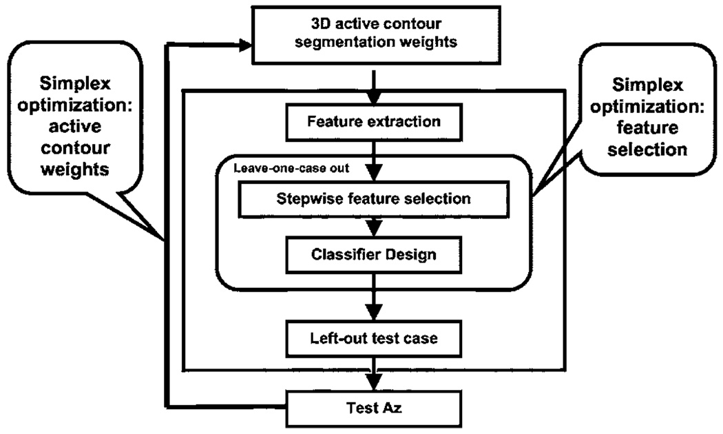
A leave-one-case-out resampling scheme was used for training the segmentation energy weights and feature selection. In a given cycle, one case that included all CT scans from the same patient was left out to be used as the test case while the other cases were used for training. The collection of the test results from all of the left-out cases after the leave-one-case-out cycles were completed was evaluated by ROC analysis.⁵¹ Two simplex optimizations were embedded: one in the determination of segmentation weights, and the other in the selection of features. Simplex optimization was used to determine the set of weights that would result in the highest A_z from the feature selection and classification step. A schematic of the training and testing process is shown in Fig. 6 and the process is described in the following.

Fig. 6.

Flow chart showing the simplex optimization process for selection of weights in the 3D AC model and classifier design.

Step 1: Initialize with a set of weights for the 3D AC.

Step 2: Generate the boundaries based on the weights, and then extract features from the boundaries.

Step 3: Perform simplex optimization for feature selection using a leave-one-case-out resampling scheme for both feature selection and classifier weight determination. The simplex searches for the F_in, F_out, and tol thresholds that provide the highest test A_z from a linear discriminant classifier with the selected features as predictor variables to differentiate the malignant and the benign classes.

Step 4: Determine a new set of AC weights using the test A_z as the FOM for the simplex optimization of AC segmentation.

Step 5: Go back to Step 2 and the subsequent steps to determine A_z for the new weights. The iteration continues until simplex converges to the best A_z or a predetermined number of iterations is performed.

In the leave-one-case-out loop for feature selection (Step 3), we also used an alternative FOM, the partial area index $A_z^{0.9}$ (TPF above 0.9) for the feature selection process. The use of $A_z^{0.9}$ as the FOM would select features that maximize the specificity at the high sensitivity region,⁵² which is often more important than having a classifier with high average sensitivity over the entire specificity range. The classifier designed with the $A_z^{0.9}$ is compared with that designed with A_z.

H. Comparison with LIDC first data set

The performance of the trained 3D AC segmentation program was evaluated with the nodules in the independent LIDC data set. We used the set of 3D AC weights that provided the highest test A_z in the leave-one-case-out training and test process using our data set as described earlier. The 3D AC weights were then fixed and applied to the LIDC nodules.

To quantify performance, we propose to use an overlap measure in combination with a percentage volume error measure. Let A denote the object segmented using the 3D AC method and L denote the gold standard reference object. Let V_A be the volume of the object A, and V_L the volume of the object L, which is the volume of the LIDC object calculated at a specified pmap threshold in this study. The overlap measure is the ratio of the intersection of volumes relative to the volume of the gold standard reference object:

$${\text{overlap}}_1(A,L)=\frac{\left|V_A\cap V_L\right|}{\left|V_L\right|}.$$ (9)

Alternatively, one may use an overlap measure that is defined as the ratio of the intersection of volumes relative to the union of the volumes of the segmented and gold standard reference objects:

$${\text{overlap}}_2(A,L)=\frac{\left|V_A\cap V_L\right|}{\left|V_A\cup V_L\right|},$$ (10)

where | · | denotes cardinality. These measures are extensions to the 3D volume from the 2D area overlap measures.^38,53 In the expressions of the overlap measures, each of the volumes can be considered as the set of voxels comprising the volume.

Overlap₁(A,L) or Overlap₂(A,L) can provide one measure of the 3D AC performance relative to the “gold standard” object but neither of them gives a complete description. Overlap₁(A,L) represents the fraction of the gold standard object that is included in the segmented object, though there is no indication as to what fraction, if any, of the segmented object is outside the gold standard object. Overlap₂(A,L) represents the fraction of overlap relative to the union, but does not provide information on how large a fraction of the gold standard object is actually included in the segmented object and whether the nonoverlap volume is contributed by the segmented object or by the gold standard.

To complement the information, we calculated the percentage volume error, V_err, defined in Eq. (11) as the difference between the volumes of the segmented object V_A and the gold standard object V_L, relative to V_L:

$$V_{\text{err}}=\frac{V_A-V_L}{V_L}\times 100\%.$$ (11)

From the two measures, Overlap₁(A,L) and V_err, one can derive a number of useful performance metrics, as detailed in Appendix B, that quantify the number of voxels correctly and incorrectly segmented as a part of the object, using the gold standard object as a reference.

I. Classification with radiologist’s feature descriptors and malignancy ratings

For comparison, we analyzed the accuracy of a classifier designed with features that were provided by the radiologists to describe the nodule characteristics. When the radiologists identified the nodule locations in each CT scan, they provided descriptors of the nodule characteristics including: (1) the longest diameter, (2) perpendicular diameter to the longest diameter, (3) conspicuity, (4) edge (smooth, lobulated, or spiculated/irregular), (5) presence or absence of calcification, (6) presence or absence of cavitation (7) presence or absence of fat, (8) attenuation (solid/mixed/ground glass opacity), (9) nodule location (the lobe of the lung), and (10) location (juxtavascular, juxtapleural). These descriptors were treated as input features to design a linear discriminant classifier. Again, leave-one-case-out resampling was used for stepwise feature selection and classifier weight determination. Simplex optimization⁵⁰ was employed to find the features that resulted in the highest test A_z.

The radiologists also provided a malignancy rating on a 5-point scale for each nodule based on subjective impression from the CT images (Fig. 2). We applied ROC analysis to the malignancy rating and estimated the A_z. This A_z value was also compared to the test A_z obtained by the computer classifier.

III. RESULTS

A. Feature selection and classification based on 3D AC

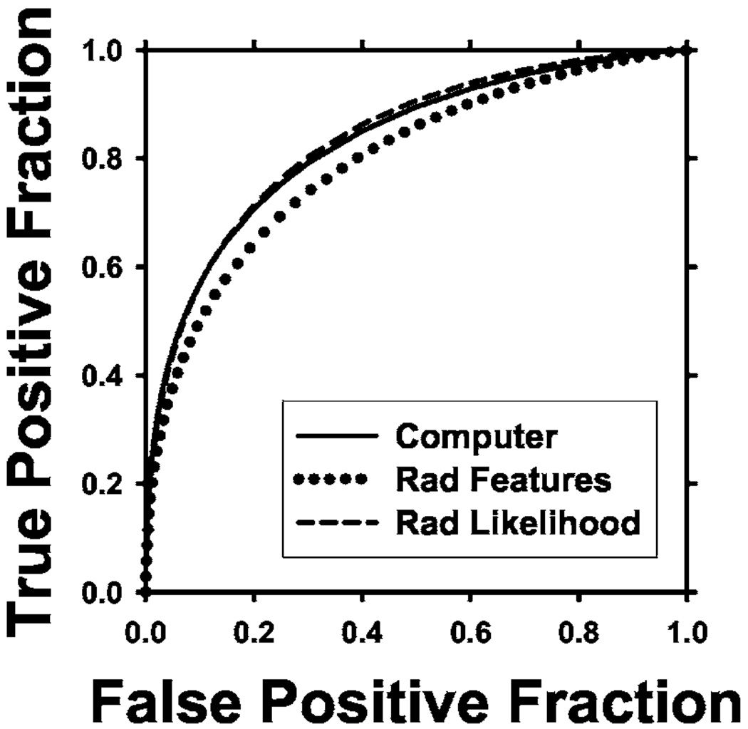
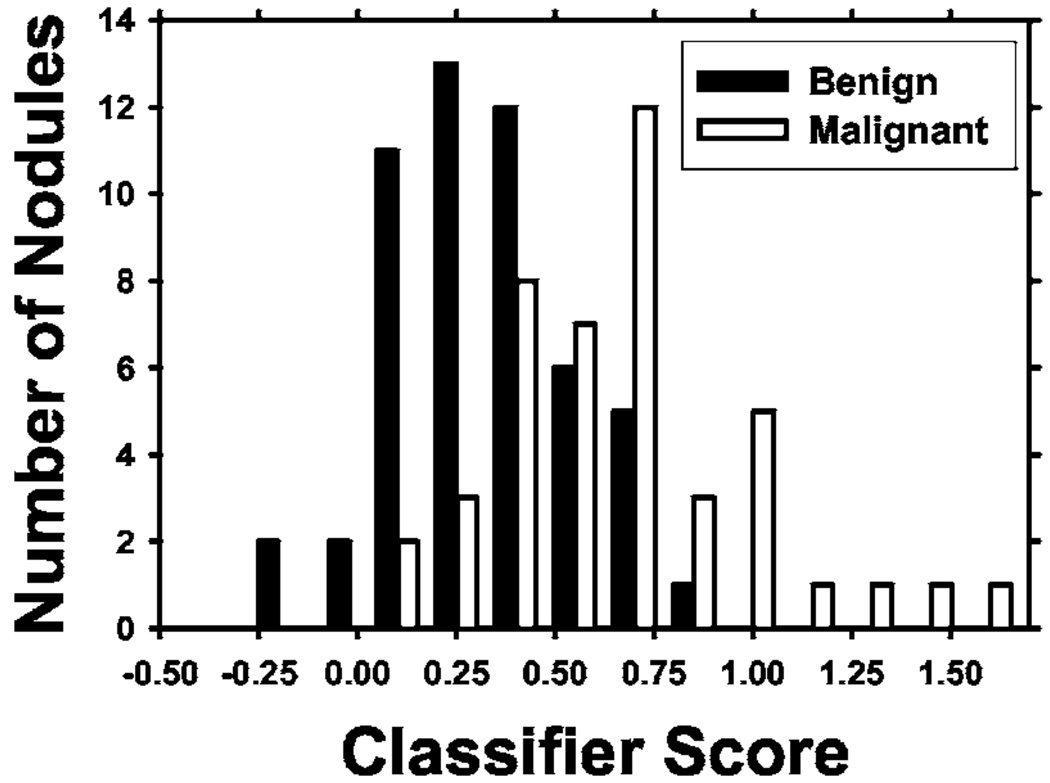
Table I shows the comparison of classification accuracy obtained with different methods. The test ROC curves for the various classifiers are shown in Fig. 7. When $A_z^{0.9}$ was used as the FOM in the leave-one-case out scheme described earlier, the training A_z was 0.88 ± 0.03 and the test A_z and $A_z^{0.9}$ were 0.78 ± 0.05 and 0.35, respectively. When A_z was used as the FOM, the training A_z was 0.87 ± 0.04 and the test A_z was 0.83 ± 0.04, with $A_z^{0.9}$ of 0.30. The difference between using $A_z^{0.9}$ and A_z as FOM was not significant (p = 0.15), as estimated by the clabroc program.⁵⁴ The distribution of classifier scores for A_z as FOM is shown in Fig. 8. An average of 4.1 features was selected. Four of the most frequently selected features along with the number of times selected out of 58 leave-one-case out cycles are:

1. (1) Long-range low gray-level emphasis on the axial planes (58).

2. (2) Run-length nonuniformity in the north-south oblique planes (56).

3. (3) Maximum CT number: (55).

4. (4) Long-range high gray-level emphasis on the axial planes (54).

This indicates that similar features were consistently selected over the different leave-one-case-out cycles, even though a different case was left out each time.

TABLE I.

Comparison of classification performance of the classifiers, in terms of A_z and $A_z^{0.9}$ obtained from leave-one-case-out testing. The classifiers were designed with different feature sets or different FOMs during simplex optimization.

	Az as FOM		$A_z^{0.9}$ as FOM
Methods	Az	$A_z^{0.9}$	Az	$A_z^{0.9}$
Computer classifier	0.83±0.04	0.30	0.78±0.05	0.35
Feature descriptors by radiologist	0.80±0.05	0.24	0.82±0.04	0.32
Likelihood of malignancy by radiologist	0.84±0.04	0.33

Fig. 7.

ROC curves comparing the different results for optimization using A_z as FOM. Computer A_z = 0.83, Rad features A_z=0.80, Rad likelihood A_z = 0.84.

Fig. 8.

Test discriminant scores of lung nodules from the leave-one-case-out segmentation training and testing method.

B. Comparison with radiologist’s feature descriptors and malignancy ratings

For classification using the radiologist-provided feature descriptors of the nodules, on average only one feature, the longest diameter, was consistently selected with A_z as the FOM. The test A_z was 0.80 ± 0.05 with $A_z^{0.9}$ of 0.24. The difference in A_z between the classifier based on radiologist-provided feature descriptors and the computer classifier did not achieve statistical significance (p = 0.40). When $A_z^{0.9}$ was used as the FOM, the test A_z and $A_z^{0.9}$ was 0.82 ± 0.04 and 0.32, respectively (p = 0.48). Using the radiologists’ malignancy ratings (Fig. 2) as input to the ROC analysis resulted in an A_z of 0.84 ± 0.04, with an $A_z^{0.9}$ of 0.33. The performance of the computer classifier was comparable to that from radiologists’ assessments of the likelihood of malignancy (p = 0.98).

C. Segmentation evaluation on LIDC data set

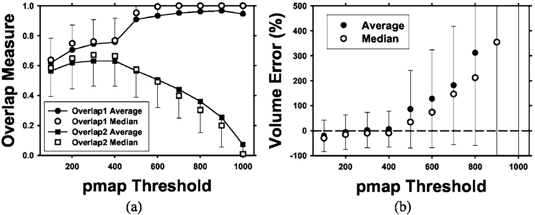
The 3D AC model with weights trained by the nodules in our data set, as described earlier, was tested on the 23 LIDC nodules. The mean and median overlap measures for the “gold standard” volumes defined at various thresholds (from 100 to 1000 in steps of 100) of the probability map (pmap) are shown in Fig. 9(a). For a given nodule, the number of voxels included within a pmap threshold, i.e., the common volume that radiologists agreed to be a part of the nodule, decreased as the pmap threshold increased. There were eight nodules with no voxels at pmap threshold of 1000 because there were no common voxels that all 18 segmentations agreed to be part of the nodule. These nodules were excluded in the calculation of Overlap₁(A,L) and the percentage volume error at pmap threshold of 1000 because the values would be undefined. The average and median were calculated with the remaining nodules. As seen in Fig. 9(a), the mean of Overlap₁(A,L) increases from 0.62 to 0.95 as the pmap increases. The median of the Overlap₁(A,L) follows a similar trend as the mean, increasing from 0.64 to 1.0. The relatively high values of Overlap₁(A,L) and its increasing trend with increasing pmap value indicate that a substantial fraction of the voxels that all radiologists marked as a part of the nodule was consistently included in the AC segmented volume. The mean of Overlap₂(A,L) ranges from 0.07 to 0.63, with the maximum at a pmap threshold of 400. The median of Overlap₂(A,L) follows a similar trend as the mean with a range from 0.009 to 0.67, reaching a maximum at the pmap threshold of 300. The small values of Overlap₂(A,L) result from the overestimation of the volumes by AC segmentation, which is also shown by the percentage volume errors.

Fig. 9.

Overlap measures (a) and volume percentage errors (b) at different pmap thresholds for testing of the 3D AC segmentation using the 23 LIDC nodules. The error bars indicate 1 s.d. from the average (only one side shown for clarity). Two overlap measures are shown: Overlap₁(A,L) relative to the gold standard volume and Overlap₂(A,L) relative to the union of the segmented volume and the gold standard volume. Note the increasing volume error as the pmap threshold increases because the LIDC-defined nodule volume decreases with increasing pmap threshold values. A pmap value of 1000 means the intersection of all 18 LIDC manually and semiautomatically drawn contours by radiologists. Eight of the nodules contain no voxels in the intersection at pmap of 1000 so that the average and the median were calculated from the remaining 15 nodules.

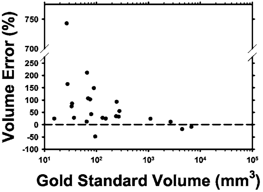
The percentage volume error relative to the radiologists’ manually segmented nodule volumes was calculated using Eq. (11) and plotted in Fig. 9(b). The average percentage volume error was lowest at a pmap threshold of 300, with a mean of 2% and a median of 10%. The volume error increased rapidly as the pmap threshold increased because the number of common voxels decreased. At pmap thresholds greater than 800, there were very few common voxels from the radiologists’ outlines so that the percentage volume error exceeded 500%. The high value of Overlap₁(A,L) indicated that most of these common voxels were included in the computer-segmented volumes. The relationship between the percentage volume error and the nodule volume calculated at the pmap threshold of 500 is plotted in Fig. 10. The threshold of 500 was chosen since at least half of the contours provided by radiologists enclosed these voxels to be a part of the true nodule.

Fig. 10.

Percentage of volume error relative to the volume (in log scale) enclosed within the contour defined by a pmap threshold of 500 for each of the 23 LIDC test nodules. One small juxta-vascular nodule had a volume error of 743% because the blood vessel was erraneously segmented.

IV. DISCUSSION

There is no ground truth for lesion boundaries in medical images. The most commonly used gold standard is subjective manual segmentation by radiologists. The LIDC studied intra- and inter-observer variability in manual segmentation of lung nodules by experienced thoracic radiologists.³³ It found large variabilities among radiologists due to the difficulty in defining the boundaries of ill-defined nodules, a task that even experienced radiologists are not required to perform clinically. The LIDC has provided a data set of 23 nodules, each with a probability map (“pmap” image) derived from 18 boundaries manually outlined by six expert thoracic radiologists (each providing one manual and two semiautomatic segmentations). The probability map can be used as the “gold standard” boundaries for evaluation of segmentation by computer methods. For our data set of nodules, we did not attempt to obtain a gold standard because even experienced radiologists have no standardized method for defining nodule boundaries. To reduce inter- and intraobserver variation, it will be necessary to have multiple radiologists segment each nodule multiple times, as done by the LIDC. This approach will be impractical to perform within one institution, since even a small data set like the one used in this study contained over 950 CT slices that intersected the nodules.

It is difficult to analytically find a set of energy weights that would provide effective segmentation for all nodules. The difficulty can be attributed to (i) energy calculations required for the linear cost function in Eq. (2) being highly nonlinear, (ii) lung nodules growing in many different irregular shapes, and (iii) boundaries between nodule and lung regions varying from very distinct to very fuzzy. One empirical method of determining the weights could be manually segmenting the lung nodules and training the contour weights to fit these case samples, using an overlap measure or distance measure as an FOM in the optimization process. However, since there are large inter-and intraobserver variabilities even among experienced thoracic radiologists as to what constitutes accurate segmentation, our overall goal is not to conform the segmented objects to subjectively estimated boundaries. Rather, the features extracted from the generated boundaries should provide accurate classification between malignant and benign nodules. We therefore used the A_z or $A_z^{0.9}$ of the feature selection step as the FOM to guide the search for the best weights in the 3D AC model. This approach not only takes into consideration classification accuracy during segmentation, it also has the advantage of eliminating the need for manually drawing the nodule boundaries by radiologists for all the training samples. Nevertheless, it would be interesting in a future study to examine how well the classifier performs if features are extracted from manually drawn contours provided by radiologists in comparison to classification by automated segmentation as described in this study.

We examined the segmentation of the nodules in the LIDC data set by our 3D AC model trained with A_z as a FOM. The average and median overlap measures at various thresholds and the percentage volume errors based on the LIDC pmap give an indication of segmentation performance. The average percentage volume errors at the pmap threshold below about 500 were in the range of −20.4% to 6.2%. The average percentage volume error at the pmap threshold of 500 was 85.7%.

The sudden increase in the values of Overlap₁(A,L) and the percentage volume error at pmap threshold of 500 was caused by the way that the boundary voxels were marked in the LIDC data set. These boundary voxels were assigned a value of 32 767 in the pmap without the original voxel values given. In our calculation of nodule volume, we included the boundary voxels to be part of the volume for pmap <500, i.e., treating the voxel values of the boundary voxels as 499. For nodule volumes at pmap threshold of greater than or equal to 500, the boundary voxels would be outside the nodule volume. This resulted in a large transition in the nodule volume at pmap threshold of 500, especially for small nodules, as shown in Fig. 9.

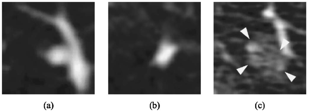
For 17 of the 23 (74%) nodules, the percentage volume error was below 100%. Three nodules had large errors. One had ground-glass opacity texture, while the other two had low contrast between the nodule and lung. Two of those were small (with longest diameters of 4.32 and 4.98 mm based on the gold standard boundaries), while the images are very noisy for the larger one. Representative slices through the center of the three lung nodules are shown in Fig. 11. These nodules contributed most to the high volume percentage error, due to incorrect segmentation of the attached blood vessels or due to incorrect expansion of the active contour beyond the faint edges.

Fig. 11.

Representative slices (not to scale) from difficult-to-segment LIDC nodules: (a) small, faint juxtavascular nodule (longest diameter 4.32 mm), (b) small nodule (longest diameter 4.98 mm), and (c) juxtavascular (longest diameter 11.92 mm) low contrast nodule in noisy image.

The 3D AC segmentation energy weights that provided the best features and A_z for nodules in our clinical data set therefore agrees to a certain extent with the boundaries perceived by radiologists in the LIDC data set. If the purpose of the segmentation is to simulate radiologists’ manual segmentation at a chosen pmap threshold, the 3D AC model should be trained with a set of nodules with gold standard boundaries at the same threshold. The 3D AC weights optimized in this manner will likely provide segmented boundaries for test nodules in better agreement with the manual boundaries than the current training. As discussed earlier, whether the boundaries that are in agreement with experienced radiologists’ manual segmentation will provide higher classification accuracy than our current segmentation method remains to be investigated. This study can be pursued when the LIDC data set is large enough to provide both training and testing samples for malignant and benign nodules.

It is generally defined and accepted that solitary pulmonary nodules are less than 3 cm in longest diameter,^55,56 but the data set used in this study included 14 masses greater than 3 cm, two of which were benign. Although one motivation for CAD tools is to assist radiologists with less-obvious (smaller) indeterminate nodules, we intend to train a CAD system that can analyze a reasonably broad range of different types of nodules and masses. We therefore included all types of nodules that we collected in the data set. We extracted morphological and gray level features in addition to texture features to be used in the input feature pool for design of our classification system. However, the stepwise feature selection with simplex optimization selected mainly texture features. This indicates that features such as the size or shape of nodules may not be as discriminatory, likely because benign objects, such as those caused by inflammatory processes, also result in nodules of varying sizes and shapes. On the other hand, the texture around benign nodules may not be the same as that caused by a malignant growth. In these cases, texture information would be more discriminatory than shape descriptors. Another indication of this is that the longest diameter feature was the one selected most consistently out of the radiologist-extracted feature space, but the same feature was not selected in the combined morphological and texture features extracted by the computer from the 3D AC boundaries. Combinations of texture features seemed to provide better discrimination, even though the longest diameter is a relatively discriminatory feature as evidenced by the A_z of 0.75 using this feature alone. Thus, we believe that the inclusion of nodules greater than 3 cm in longest axis would provide the texture information important for training, not necessarily for size or shape, and that the trained CAD system may be used for analysis of nodules or masses over a reasonably broad range of sizes because its performance does not depend on the size of the nodule or masses.

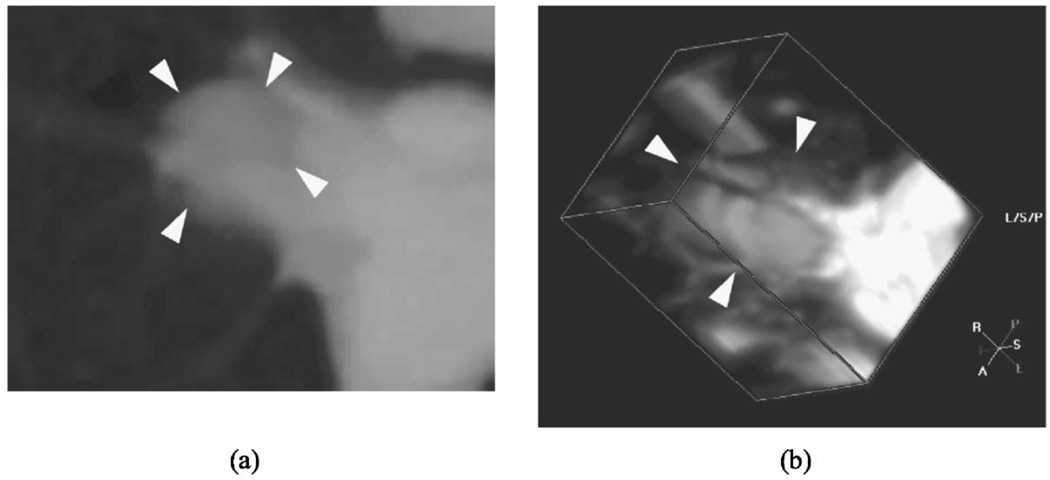
There were nodules for which the classifier did not perform well. One example is shown in Fig. 12. This nodule was malignant, but the classifier gave a score indicating a low likelihood of malignancy. This nodule was embedded and located between branching blood vessels near the lung hilum, which resulted in poor segmentation [Overlap₁(A,L) measure of 0.67 and 78% volume error]. Furthermore, the texture features extracted from this nodule would not be a good indicator of spiculation or malignant growth, because the blood vessels occupied much of the surrounding tissue volume. Even though our segmentation method is fairly robust with juxtavascular nodules, an embedded nodule among large pulmonary vessels presents a difficult case. Improved segmentation methods utilizing information such as vessel tracking to remove vessels and new features will have to be investigated in future studies.

Fig. 12.

An example of a nodule which was difficult to segment because it was embedded in thick blood vessels, leading to inaccurate classification. (a) axial slice through the nodule, and (b) 3D volume containing the nodule.

We are improving our current method by expanding our data set and analyzing the classification performance of different types of nodules. For example, nodules from primary lung cancer may have different characteristics than metastatic nodules, although both types would be considered malignant. Our long-term goal is to aid the differentiation of malignant and benign nodules detected in screening, making identification of primary lung cancer of prime importance. Thus, training classifiers that are specific to the features of primary lung cancer may improve the performance of the classifier in the screening population.

Another aspect of our current system that needs improvement is the method to determine which object is the nodule in the VOI. Currently we choose the largest object close to the center, since the VOIs were marked by radiologists. However, if a combined detection and classification system is to be developed in the future, the VOI may not center at the automatically detected object, and the object may not be the largest one in the VOI. More intelligent methods for differentiating nodules from other normal lung structures in the VOI segmented by clustering will have to be investigated.

Although the use of leave-one-case-out validation results is a commonly accepted approach in CAD literature because of the difficulty of collecting a large enough database for training, validation, and independent testing, it is prudent to keep in mind that the performance of the CAD system may not be considered generalizable to the patient population until its performance is verified with a truly independent test set that is not seen by the CAD system or the trainer during the developmental process. Our test results show comparable performance between CAD and radiologists’ assessment of the likelihood of malignancy of the nodules. In a clinical situation, radiologists may be able to utilize other information such as patient history and clinical data, in addition to image data, to assess the likelihood of malignancy. An advanced CAD system may also merge all available information into a diagnostic recommendation. At the current stage, we focus on optimizing the use of image data to extract diagnostic information to avoid the masking of the image information by other dominant risk factors such as smoking history or age. Further, CAD is not intended to be used as a stand-alone diagnostic tool. After an effective classifier is designed, it is necessary to determine whether radiologists would improve their classification of lung nodules with CAD.

V. CONCLUSION

Our results demonstrate that 3D AC can segment lung nodules automatically. Automated feature extraction from the segmented boundary and classification can achieve an accuracy comparable to that of an experienced radiologist. The computer classifier thus has the potential to provide a second opinion to radiologists for assessing the likelihood of malignancy of a lung nodule. When the 3D AC trained with our clinical data set was applied to the LIDC data set, the segmented volumes by the computer algorithm were in general larger than those manually segmented by the radiologists. It remains to be investigated whether the 3D AC model trained using gold standard boundaries at a given threshold such as those provided by the LIDC database can achieve higher classification accuracy than that achieved with our current approach. Comparison of the two approaches will be pursued when a large data set is available in the LIDC database.

APPENDIX A

RLS FEATURES

The Gallaway run-length features are described in the following, where p(i, j) is the run-length matrix that stores information on the number of runs with pixels of gray-level i and run length j. M is the number of gray levels, N is the number of runs, n_r is the total number of runs, and n_p is the number of pixels in the image.

• Short Runs Emphasis (SRE):

  $$\text{SRE}=\frac{1}{n_r}{\displaystyle \sum _{i=1}^M{\displaystyle \sum _{j=1}^N\frac{p(i,j)}{j^2}.}}$$ (A1)
• Long Runs Emphasis (LRE):

  $$\text{LRE}=\frac{1}{n_r}{\displaystyle \sum _{i=1}^M{\displaystyle \sum _{j=1}^{N}p(i,j)·j^2.}}$$ (A2)
• Gray-Level Nonuniformity (GLN):

  $$\text{GLN}=\frac{1}{n_r}{{\displaystyle \sum _{i=1}^M\left({\displaystyle \sum _{j=1}^{N}p(i,j)}\right)}}^2.$$ (A3)
• Run Length Nonuniformity (RLN):

  $$\text{RLN}=\frac{1}{n_r}{{\displaystyle \sum _{j=1}^N\left({\displaystyle \sum _{i=1}^{M}p(i,j)}\right)}}^2.$$ (A4)
• Run Percentage (RP):

  $$\text{RP}=\frac{n_r}{n_p}.$$ (A5)

Dasarathy and Holder presented four more features.⁴⁸ These are based on the idea of joint statistical measures of the gray levels and run length.

• Short Run Low Gray-Level Emphasis (SRLGE):

  $$\text{SRLGE}=\frac{1}{n_r}{\displaystyle \sum _{i=1}^M{\displaystyle \sum _{j=1}^N\frac{p(i,j)}{i^2·j^2}.}}$$ (A6)
• Short Run High Gray-Level Emphasis (SRHGE):

  $$\text{SRHGE}=\frac{1}{n_r}{\displaystyle \sum _{i=1}^M{\displaystyle \sum _{j=1}^N\frac{p(i,j)·i^2}{j^2}.}}$$ (A7)
• Long Run Low Gray-Level Emphasis (LRLGE):

  $$\text{LRLGE}=\frac{1}{n_r}{\displaystyle \sum _{i=1}^M{\displaystyle \sum _{j=1}^N\frac{p(i,j)·j^2}{i^2}.}}$$ (A8)
• Long Run High Gray-Level Emphasis (LRHGE):

  $$\text{LRLGE}=\frac{1}{n_r}{\displaystyle \sum _{i=1}^M{\displaystyle \sum _{j=1}^{N}p(i,j)·i^2·j^2.}}$$ (A9)

APPENDIX B

SEGMENTATION PERFORMANCE METRICS

By combining the overlap measure Overlap₁(A,L) in Eq. (9) and the percentage volume error (V_err) in Eq. (11), one can define a number of performance metrics that quantify the number of voxels correctly and incorrectly segmented as a part of the object, using the gold standard object as a reference.

True positive fraction (TPF): the fraction of the voxels that are in the gold standard object and are included in the segmented object:

$$\text{TPF}={\text{Overlap}}_1(A,L).$$ (B1)

False positive ratio (FPR): the ratio of the voxels that are in the segmented object but not in the gold standard object, relative to the gold standard object:

$$\text{FPR}=V_{\text{err}}+[1-{\text{Overlap}}_1(A,L)].$$ (B2)

False negative fraction (FNF): the fraction of the voxels that are in the gold standard object but not included in the segmented object:

$$\text{FNF}=1-{\text{Overlap}}_1(A,L).$$ (B3)

Nonoverlapping volume ratio (NOVR): the ratio of voxels in the gold standard object and in the segmented object that do not overlap, relative to the gold standard object:

$$\text{NOVR}=V_{\text{err}}+2[1-{\text{Overlap}}_1(A,L)]=\text{FPR}+\text{FNF}.$$ (B4)

The equations above use Overlap₁(A,L), but the conventional overlap measure in Eq. (10) can also be expressed in terms of Overlap₁(A,L) and NOVR:

$${\text{Overlap}}_2(A,L)=\frac{{\text{Overlap}}_1(A,L)}{\text{NOVR}+{\text{Overlap}}_1(A,L)}\text{.}$$ (B5)

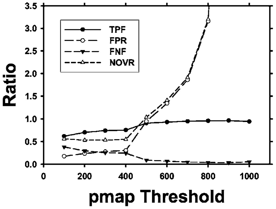
Therefore, the two measures Overlap₁(A,L) and V_err provide a complete description of the segmentation performance. As an example, we have plotted the metrics described above in Fig. 13 as derived from the average Overlap₁(A,L) and V_err values for the LIDC nodules shown in Fig. 9.

Fig. 13.

The performance metrics TPF, FPR, FNF, and NOVR derived from the average Overlap₁(A,L) and V_err measures shown in Fig. 9.

From Eq. (B5), it is seen that Overlap₁(A,L) can be expressed in terms of Overlap₂(A,L):

$$\text{TPF}={\text{Overlap}}_1(A,L)=\frac{{\text{Overlap}}_2(A,L)·(V_{\text{err}}+2)}{1+{\text{Overlap}}_2(A,L)}$$ (B6)

and thus Overlap₂(A,L) in conjunction with V_err can also provide similar performance metrics defined above, although the relationships are more involved. These analyses indicate that it is important to include the percentage volume error as a complement to either of the overlap measures.

References

- 1.American Cancer Society. Cancer Facts & Figures. 2005 www.cancer.org2005.
- 2.Swensen SJ, Viggiano RW, Midthun DE, Müller NL, Sherrick A, Yamashita K, Naidich DP, Patz EF, Hartman TE, Muhm JR, et al. Lung nodule enhancement at CT: Multicenter study. Radiology. 2000;214:73–80. doi: 10.1148/radiology.214.1.r00ja1473. [DOI] [PubMed] [Google Scholar]
- 3.Henschke CI, McCauley DI, Yankelevitz DF, Naidich DP, McGuinness G, Miettinen OS, Libby DM, Pasmantier MW, Koizumi J, Altorki NK, et al. Early lung cancer action project: Overall design and findings from baseline screening. Lancet. 1999;354:99–105. doi: 10.1016/S0140-6736(99)06093-6. [DOI] [PubMed] [Google Scholar]
- 4.Diederich S, Wormanns D, Semik M, Thomas M, Lenzen H, Roos N, Heindel W. Screening for early lung cancer with low-dose spiral CT: Prevalence in 817 asymptomatic smokers. Radiology. 2002;222:773–781. doi: 10.1148/radiol.2223010490. [DOI] [PubMed] [Google Scholar]
- 5.Kaneko M, Eguchi K, Ohmatsu H, Kakinuma R, Naruke T, Suemasu K, Moriyama N. Peripheral lung cancer: Screening and detection with low-dose spiral CT versus radiography. Radiology. 1996;201:798–802. doi: 10.1148/radiology.201.3.8939234. [DOI] [PubMed] [Google Scholar]
- 6.Nawa T, Nakagawa T, Kusano S, Kawasaki Y, Sugawara Y, Nakata H. Lung cancer screening using low-dose spiral CT: Results of baseline and 1-year follow-up studies. Chest. 2002;122:15–20. doi: 10.1378/chest.122.1.15. [DOI] [PubMed] [Google Scholar]
- 7.Sone S, Takashima S, Li F, Yang F, Honda T, Maruyama Y, Hasega M, Yamanda T, Kubo K, Hanamura K, et al. Mass screening for lung cancer with mobile spiral computed tomography scanner. Lancet. 1998;352:1242–1245. doi: 10.1016/S0140-6736(97)08229-9. [DOI] [PubMed] [Google Scholar]
- 8.Sone S, Li F, Yang ZG, Honda T, Maruyama Y, Takashima S, Hasegawa M, Kawakami S, Kubo K, Haniuda KM, et al. Results of three-year mass screening programme for lung cancer using mobile low-dose spiral computed tomography scanner. Br. J. Cancer. 2001;84:25–32. doi: 10.1054/bjoc.2000.1531. [DOI] [PMC free article] [PubMed] [Google Scholar]
- 9.Swensen SJ, Jett JR, Hartman TE, Midthun DE, Mandrekar SJ, Hillman SL, Sykes A-M, Aughenbaugh GL, Allen AOBL. CT screening for lung cancer: Five-year prospective experience. Radiology. 2005;235:259–265. doi: 10.1148/radiol.2351041662. [DOI] [PubMed] [Google Scholar]
- 10.Swensen SJ, Jett JR, Hartman TE, Midthun DE, Sloan JA, Sykes AM, Aughenbaugh GL, Clemens MA. Lung cancer screening with CT: Mayo Clinic experience. Radiology. 2003;226:756–761. doi: 10.1148/radiol.2263020036. [DOI] [PubMed] [Google Scholar]
- 11.Freer TW, Ulissey MJ. Screening mammography with computer-aided detection: Prospective study of 12,860 patients in a community breast center. Radiology. 2001;220:781–786. doi: 10.1148/radiol.2203001282. [DOI] [PubMed] [Google Scholar]
- 12.Armato SG, Giger ML, Moran CJ, Blackburn JT, Doi K, MacMahon H. Computerized detection of pulmonary nodules on CT scans. Radiographics. 1999;19:1303–1311. doi: 10.1148/radiographics.19.5.g99se181303. [DOI] [PubMed] [Google Scholar]
- 13.Brown MS, McNitt-Gray MF, Goldin JG, Suh RD, Sayre JW, Aberle DR. Patient-specific models for lung nodule detection and surveillance in CT images. IEEE Trans. Med. Imaging. 2001;20:1242–1250. doi: 10.1109/42.974919. [DOI] [PubMed] [Google Scholar]
- 14.Croisille P, Souto M, Cova M, Wood S, Afework Y, Kuhlman JE, Zerhouni EA. Pulmonary nodules: Improved detection with vascular segmentation and extraction with spiral CT. Radiology. 1995;197:397–401. doi: 10.1148/radiology.197.2.7480683. [DOI] [PubMed] [Google Scholar]
- 15.Malladi R, Sethian JA, Vemuri BC. Shape modeling with front propagation: A level set approach. IEEE Trans. Pattern Anal. Mach. Intell. 1995;17:158–175. [Google Scholar]
- 16.Yang J, Staib LH, Duncan JS. Neighbor-constrained segmentation with level set based 3-D deformable models. IEEE Trans. Med. Imaging. 2004;23:940–948. doi: 10.1109/TMI.2004.830802. [DOI] [PMC free article] [PubMed] [Google Scholar]
- 17.Cuadra MB, Pollo C, Bardera A, Cuisenaire O, Villemure J-G, Thiran J-P. Atlas-based segmentation of pathological MR brain images using a model of lesion growth. IEEE Trans. Med. Imaging. 2004;23:1301–1314. doi: 10.1109/TMI.2004.834618. [DOI] [PubMed] [Google Scholar]
- 18.Gurcan MN, Sahiner B, Petrick N, Chan HP, Kazerooni EA, Cascade PN, Hadjiiski L. Lung nodule detection on thoracic computed tomography images: Preliminary evaluation of a computer-aided diagnosis system. Med. Phys. 2002;29:2552–2558. doi: 10.1118/1.1515762. [DOI] [PubMed] [Google Scholar]
- 19.Brown MS, Goldin JG, Suh RD, McNitt-Gray MF, Sayre JW, Aberle DR. Lung micronodules: Automated method for detection at thin-section CT—nitial experience. Radiology. 2003;226:256–262. doi: 10.1148/radiol.2261011708. [DOI] [PubMed] [Google Scholar]
- 20.Kim KG, Goo JM, Kim JH, Lee HJ, Min BG, Bae KT, Im J-G. Computer-aided diagnosis of localized ground-glass opacity in the lung at CT: Initial experience. Radiology. 2005;237:657–661. doi: 10.1148/radiol.2372041461. [DOI] [PubMed] [Google Scholar]
- 21.Armato S, Li F, Giger M, MacMahon H, Sone S, Doi K. Lung-cancer: Performance of automated lung nodule detection applied to cancers missed in a CT screening program. Radiology. 2002;225:685–692. doi: 10.1148/radiol.2253011376. [DOI] [PubMed] [Google Scholar]
- 22.Bae KT, Kim J-S, Na Y-H, Kim KG, Kim J-H. Pulmonary nodules: Automated detection on CT images with morphologic matching algorithm—preliminary results. Radiology. 2005;236:286–293. doi: 10.1148/radiol.2361041286. [DOI] [PubMed] [Google Scholar]
- 23.Lee Y, Hara T, Fujita H, Itoh S, Ishigaki T. Automated detection of pulmonary nodules in helical CT images based on an improved template-matching technique. IEEE Trans. Med. Imaging. 2001;20:595–604. doi: 10.1109/42.932744. [DOI] [PubMed] [Google Scholar]
- 24.Kanazawa K, Kawata Y, Niki N, Satoh H, Ohmatsu H, Kakinuma R, Kaneko M, Moriyama N, Eguchi K. Computer-aided diagnosis for pulmonary nodules based on helical CT images. Comput. Med. Imaging Graph. 1998;22:157–167. doi: 10.1016/s0895-6111(98)00017-2. [DOI] [PubMed] [Google Scholar]
- 25.Suzuki K, Armato S, Li F, Sone S, Doi K. Massive training artificial neural network (MTANN) for reduction of false positives in computerized detection of lung nodules in low-dose computed tomography. Med. Phys. 2003;30:1602–1617. doi: 10.1118/1.1580485. [DOI] [PubMed] [Google Scholar]
- 26.McNitt-Gray MF, Hart EM, Wyckoff N, Sayre JW, Goldin JG, Aberle DR. A pattern classification approach to characterizing solitary pulmonary nodules imaged on high resolution CT: Preliminary results. Med. Phys. 1999;26:880–888. doi: 10.1118/1.598603. [DOI] [PubMed] [Google Scholar]
- 27.Shah SK, McNitt-Gray MF, Rogers SR, Goldin JG, Suh RD, Sayre JW, Petkovska I, Kim HJ, Aberle DR. Computer-aided diagnosis of the solitary pulmonary nodule. Acad. Radiol. 2005;12:570–575. doi: 10.1016/j.acra.2005.01.018. [DOI] [PubMed] [Google Scholar]
- 28.Armato SG, Altman MB, Wilkie J. Automated lung nodule classification following automated nodule detection on CT: A serial approach. Med. Phys. 2003;30:1188–1197. doi: 10.1118/1.1573210. [DOI] [PubMed] [Google Scholar]
- 29.Kawata Y, Niki N, Ohmatsu H, Kakinuma R, Eguchi K, Kaneko M, Moriyama N. Quantitative surface characterization of pulmonary nodules based on thin-section CT images. IEEE Trans. Nucl. Sci. 1998;45:2132–2138. [Google Scholar]
- 30.Li F, Aoyama M, Shiraishi J, Abe H, Li Q, Suzuki K, Engelmann R, Sone S, MacMahon H, Doi AK. Radiologists’ performance for differentiating benign from malignant lung nodules on high-resolution CT using computer-estimated likelihood of malignancy. AJR, Am. J. Roentgenol. 2004;183:1209–1215. doi: 10.2214/ajr.183.5.1831209. [DOI] [PubMed] [Google Scholar]
- 31.Aoyama M, Li Q, Katsuragawa S, Li F, Sone S, Doi K. Computerized scheme for determination of the likelihood measure of malignancy for pulmonary nodules on low-dose CT images. Med. Phys. 2003;30:387–394. doi: 10.1118/1.1543575. [DOI] [PubMed] [Google Scholar]
- 32.Suzuki K, Li F, Sone S, Doi K. Computer-aided diagnostic scheme for distinction between benign and malignant nodules in thoracic low-dose CT by use of massive training artificial neural network. IEEE Trans. Med. Imaging. 2005;24:1138–1150. doi: 10.1109/TMI.2005.852048. [DOI] [PubMed] [Google Scholar]
- 33.Armato SG, McLennan G, McNitt-Gray MF, Meyer CR, Yankelevitz D, Aberle DR, Henschke CI, Hoffman EA, Kazerooni EA, MacMahon H, et al. Lung image database consortium: Developing a resource for the medical imaging research community. Radiology. 2004;232:739–748. doi: 10.1148/radiol.2323032035. [DOI] [PubMed] [Google Scholar]
- 34.Sahiner B, Chan HP, Petrick N, Wei D, Helvie MA, Adler DD, Goodsitt MM. Image feature selection by a genetic algorithm: Application to classification of mass and normal breast tissue on mammograms. Med. Phys. 1996;23:1671–1684. doi: 10.1118/1.597829. [DOI] [PubMed] [Google Scholar]
- 35.Kass M, Witkin A, Terzopoulos D. Snakes: active contour models. Int. J. Comput. Vis. 1987;1:321–331. [Google Scholar]
- 36.Williams DJ, Shah M. A fast algorithm for active contours and curvature estimation. CVGIP: Image Understand. 1992;55:14–26. [Google Scholar]
- 37.Poon CS, Braun M. Image segmentation by a deformable contour model incorporating region analysis. Phys. Med. Biol. 1997;42:1833–1841. doi: 10.1088/0031-9155/42/9/013. [DOI] [PubMed] [Google Scholar]
- 38.Sahiner B, Petrick N, Chan HP, Hadjiiski LM, Paramagul C, Helvie MA, Gurcan MN. Computer-aided characterization of mammo-graphic masses: Accuracy of mass segmentation and its effects on characterization. IEEE Trans. Med. Imaging. 2001;20:1275–1284. doi: 10.1109/42.974922. [DOI] [PubMed] [Google Scholar]
- 39.Cohen LD. On active contour models and balloons. CVGIP: Image Understand. 1991;53:211–218. [Google Scholar]
- 40.Way TW, Sahiner B, Hadjiiski L, Chan H-P, Bogot N, Cascade P, Kazerooni E, Fessler JA. Segmentation of pulmonary nodules with 3D active contour model for computer-aided diagnosis. Radiological Society of North America Scientific Assembly and Annual Meeting Program; Oakbrook, IL. RSNA; November 30–December 5; Chicago, IL: 2003. [Google Scholar]
- 41.Kostis WJ, Reeves AP, Yankelevitz DF, Henschke CI. Three-dimensional segmentation and growth-rate estimation of small pulmonary nodules in helical CT images. IEEE Trans. Med. Imaging. 2003;22:1259–1274. doi: 10.1109/TMI.2003.817785. [DOI] [PubMed] [Google Scholar]
- 42.Gurney JW. Determining the likelihood of malignancy in solitary pulmonary nodules with Bayesian analysis, I. Theory. Radiology. 1993;186:405–413. doi: 10.1148/radiology.186.2.8421743. [DOI] [PubMed] [Google Scholar]
- 43.Erasmus JJ, Connolly JE, McAdams HP, Roggli VL. Solitary pulmonary nodules. I. Morphological evaluation for differentiation of benign and malignant lesions. Radiographics. 2000;20:43–58. doi: 10.1148/radiographics.20.1.g00ja0343. [DOI] [PubMed] [Google Scholar]
- 44.Siegelman S, Khouri N, Scott JWW, Leo F, Hamper U, Fishman E, Zerhouni E. Pulmonary hamartoma: CT findings. Radiology. 1986;160:313–317. doi: 10.1148/radiology.160.2.3726106. [DOI] [PubMed] [Google Scholar]
- 45.Ledor K, Fish B, Chaise L, Ledor S. CT diagnosis of pulmonary hamartomas. J. Comput. Assist. Tomogr. 1981;5:343–344. doi: 10.1016/0149-936x(81)90075-8. [DOI] [PubMed] [Google Scholar]
- 46.Sahiner B, Chan HP, Petrick N, Helvie MA, Goodsitt MM. Computerized characterization of masses on mammograms: The rubber band straightening transform and texture analysis. Med. Phys. 1998;25:516–526. doi: 10.1118/1.598228. [DOI] [PubMed] [Google Scholar]
- 47.Galloway MM. Texture classification using gray level run lengths. Comput. Graph. Image Process. 1975;4:172–179. [Google Scholar]
- 48.Dasarathy BR, Holder EB. Image characterizations based on joint gray-level run-length distributions. Pattern Recogn. Lett. 1991;12:497–502. [Google Scholar]
- 49.Chan HP, Wei D, Helvie MA, Sahiner B, Adler DD, Goodsitt MM, Petrick N. Computer-aided classification of mammo-graphic masses and normal tissue: Linear discriminant analysis in texture feature space. Phys. Med. Biol. 1995;40:857–876. doi: 10.1088/0031-9155/40/5/010. [DOI] [PubMed] [Google Scholar]
- 50.Spendley W, Hext GR, Himsworth FR. Sequential application of simplex designs in optimization and evolutionary operation. Technometrics. 1962;4:441–461. [Google Scholar]
- 51.Metz CE. ROC methodology in radiologic imaging. Invest. Radiol. 1986;21:720–733. doi: 10.1097/00004424-198609000-00009. [DOI] [PubMed] [Google Scholar]
- 52.Sahiner B, Chan HP, Petrick N, Helvie MA, Goodsitt MM. Design of a high-sensitivity classifier based on a genetic algorithm: Application to computer-aided diagnosis. Phys. Med. Biol. 1998;43:2853–2871. doi: 10.1088/0031-9155/43/10/014. [DOI] [PubMed] [Google Scholar]
- 53.Goodsitt MM, Chan HP, Lydick JT, Gandra CR, Chen NG, Helvie MA, Bailey J, Roubidoux MA, Blane CE, Sahiner B, et al. An observer study comparing spot imaging regions selected by radiologists and a computer for an automated stereo spot mammography technique. Med. Phys. 2004;31:1558–1567. doi: 10.1118/1.1737492. [DOI] [PubMed] [Google Scholar]
- 54.Metz CE, Herman BA, Shen JH. Maximum-likelihood estimation of receiver operating characteristic (ROC) curves from continuously-distributed data. Stat. Med. 1998;17:1033–1053. doi: 10.1002/(sici)1097-0258(19980515)17:9<1033::aid-sim784>3.0.co;2-z. [DOI] [PubMed] [Google Scholar]
- 55.Tan BB, Flaherty KR, Kazerooni EA, Iannettoni MD. The solitary pulmonary nodule. Chest. 2003;123:89–96. doi: 10.1378/chest.123.1_suppl.89s. [DOI] [PubMed] [Google Scholar]
- 56.Ost D, Fein A. Evaluation and management of the solitary pulmonary nodule. Am. J. Respir. Crit. Care Med. 2000;162:782–787. doi: 10.1164/ajrccm.162.3.9812152. [DOI] [PubMed] [Google Scholar]