

SYNOPSIS
Objectives.
Although numerous studies have examined health-related quality of life (HRQOL) longitudinally, little is known about the impact of seasonality on HRQOL. We examined trend and seasonal variations of population HRQOL.
Methods.
We used data from the monthly Behavioral Risk Factor Surveillance System (BRFSS). We examined monthly observed mean physically and mentally unhealthy days from January 1993 to December 2006, using the structural time-series model to estimate the trend and seasonality of HRQOL.
Results.
We found overall worsening physical and mental health during the time period and a significant and regular seasonal pattern in both physical and mental health. The worst physical health was during the winter and the best physical health was during the summer. The mean number of physically unhealthy days in January was 0.63 days higher than in July. The worst mental health occurred during the spring and fall, but the magnitude of the seasonal effect was much smaller. The difference between the best and worst months of mentally unhealthy days was approximately 0.23 days. We found significant differences in unadjusted and season-adjusted unhealthy days in many counties.
Conclusions.
Our findings can be used to examine time-varying causal factors and the impact of interventions, such as policies designed to improve population health. Our findings also demonstrated the need for calculating season-adjusted HRQOL scores when examining cross-sectional factors on the population HRQOL measures for continuous surveys or longitudinal data.
Measures of health-related quality of life (HRQOL) have been used with greater frequency to assess relevant outcomes for populations.1–5 Like mortality and morbidity statistics, population HRQOL data are collected regularly from national and local health surveys,1,6,7 and summary statistics of HRQOL scores are used as community health indicators to track health needs for target subgroups and elucidate health disparities.1,4,8,9 Longitudinal data of HRQOL measures may be used to monitor progress with regard to the Healthy People goals and assist in analyzing the effectiveness of interventions to improve health in selected groups.1,3–5
Although numerous studies have examined HRQOL longitudinally, little is known about the impact of seasonality on HRQOL.4,5 By contrast, seasonal variations in mortality and morbidity statistics have been reported in the literature for conditions impacting both physical and mental health.10–12 Health statistics measured at multiple time points include time-series variations and cross-sectional variations. Estimating time-series variations, such as trend and seasonality, can enable the exploration of causal effects.13 However, when analyzing data from continuous surveys or longitudinal studies, trend and seasonal variations may be large enough to conceal true patterns of data.
When comparing data from different communities and years, the time of year during which data are collected can affect respondents' health status. For example, changes of season and, in particular, the shortening hours of sunlight may be associated with changes in mood and behavior.14,15 Additionally, substantial seasonal variation of self-reported leisure time physical activity has been noted, and seasonal variation in activity levels may play a role in the relationship between physical activity and cardiovascular disease.16 Therefore, analysis of HRQOL data without adjusting for such effects may not be accurate and appropriate adjustment may be necessary.12
Since 1993, the Behavioral Risk Factor Surveillance System (BRFSS), a monthly population-based health survey of the U.S. adult population, has incorporated a set of HRQOL survey instruments called the Healthy Days measures.1 Data from the BRFSS have been used to track trends of population HRQOL over time and provide estimates for all states and some sub-state areas.17 A recent examination of monthly mean unhealthy days from 1998 to 2001 among U.S. adults using BRFSS data found an annual recurrence of worse physically unhealthy days during winter after random disturbance was smoothed out using a three-month moving average.4 However, no clear periodic pattern was observed in mentally unhealthy days. Further removal of random disturbance by combining multiple years' data to obtain the mean monthly score for each year still yielded inconclusive results.4,5 However, direct estimates of seasonality that fail to adjust for the time trend effect can be biased. For example, if data had an upward trend, monthly estimates of HRQOL scores would be too low in January and too high in December. Additionally, because the seasonal patterns may change from year to year, using the mean seasonal effect from combining multiple years of data would be inaccurate.4,5,18–22 Furthermore, estimating trend and seasonality should adjust for changes in population demographics over time.
This study examined some time-varying variations, including the trend or the long-term upward or downward tendency, seasonality or the periodic recurring annually, and correlations with time-varying factors of HRQOL data. If the variables of interest are cross-sectional alone, a conventional approach is the hierarchic longitudinal models.18 When the variables of interest are time-series effects, such an approach is difficult because effect sizes are stochastic and extensive time index parameters would be required in the hierarchic longitudinal models.18,19 By contrast, the time-series analysis methods provide a flexible alternative for estimating trend and seasonality, allowing these time-series effects to vary stochastically over time using only a few parameters. One of the time-series methods, the structural time-series model, decomposes observed data series into interpretable, unobserved components, such as trend, seasonality, and random disturbance. This model-based approach is particularly relevant because it can capture the feature of each decomposed component.20,21 It also has the flexibility to examine the impact of additional time-varying variables on HRQOL.18,20,21,23
In this study, we examined the trend and seasonality of population physically and mentally unhealthy days to calculate season-adjusted HRQOL scores for tracking changes in population health and making comparisons between subgroups (e.g., community-to-community or peer comparisons). We applied the structural time-series models to the monthly mean unhealthy days. We also examined the model's ability to capture factors and interventions that might affect HRQOL scores.
METHODS
Data sources and measures
We used monthly HRQOL data from the 1993–2006 BRFSS, the largest continuously conducted health survey of noninstitutional civilian residents in the U.S. The survey generates population-based samples from each of the 50 states and the District of Columbia.17,24 Respondents were asked about the number of days in the past 30 days that their physical and mental health were not good, respectively (physically and mentally unhealthy days).1
Although the BRFSS data were designed to be collected on a monthly basis in each state, there are some month-to-month differences in sample sizes for some sub-state areas due to the multistage stratified design of the BRFSS. Even at the state level, there is evidence of such differences. For example, in 2004, Connecticut interviewed only 6.8% of respondents during the first quarter but nearly half of total respondents (43.3%) during the second quarter. At the sub-state level, such variation is even larger.
Statistical analysis
Our analyses examined the observed mean physically and mentally unhealthy days during a period of 168 months from January 1993 to December 2006 (Figure 1). The structural time-series model decomposed the observed mean physically and mentally unhealthy days at month t, yt, into trend (μt), season (γt), regression (
 |
), and random disturbance (εt) components:20,21
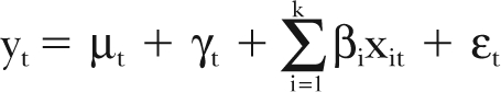 |
Figure 1.
Monthly mean physically and mentally unhealthy days: 1993–2006 BRFSS
BRFSS = Behavioral Risk Factor Surveillance System

The trend component μt is fitted as a locally linear trend model, in which the current value equals the previous value plus a time-varying slope κt and an independent random normal disturbance ηt:
 |
where ξt ∼ N(0, σξ2 is the independent random normal disturbance of slope.
The regression component
 |
is used to examine for correlations between time-varying covariates.20,21 Here, xt = (x1t , x2t ,…,xkt) is a set of k number of time-varying independent variables and is fitted into a multiple linear regression. We used the regression for two purposes. First, the regression adjusted for some potential confounders for estimating trend and seasonality. In this analysis, we included the monthly proportion of the population in each age, race/ethnicity, and gender category in the model to adjust for population demographic changes over time. Second, the regression estimated the impact of an intervention at time t0 on observed scores, adjusting for trend and seasonality. We estimated the short- and long-term impacts of the intervention by introducing two dummy intervention variables:
 |
We used the intervention variable x1 to estimate the short-term effect from time t0 to t0 + L and the intervention variable x2 to estimate the long-term effect and possible delayed effect (d ≥ 0) after time t0 + d. As an example of this application, we estimated the short- and long-term impacts of the September 11, 2001, attacks on mentally unhealthy days.
The variances of the disturbance terms (σε2, ση2, σξ2, and σω2) were estimated using the algorithms by maximizing likelihood function numerically. Each component of the structure time-series model was estimated using the Kilman filter, a recursive algorithm that minimizes the mean square error.20,21 We calculated the season-adjusted HRQOL scores by subtracting the seasonal effect from the observed monthly data.
RESULTS
We estimated trend and seasonal effects of physically and mentally unhealthy days from 1993 to 2006 and adjusted all estimates for demographics (age, race/ethnicity, and gender). Figure 1 presents the monthly mean physically and mentally unhealthy days during this time period. Because our analysis showed that the seasonal effects were stable over the years, we reported the seasonal effect only in the final cycle of the series (Figure 2).
Figure 2.
Seasonal difference in mean physically and mentally unhealthy days, 2006
BRFSS = Behavioral Risk Factor Surveillance System

The results showed a strong and significant seasonal impact on physically unhealthy days. In particular, the worst physical health occurred during the winter and the best physical health occurred during the summer. The mean number of physically unhealthy days in the worst month was 0.63 days higher than for the best month (p<0.0001; range: −0.30 to +0.33 days; standard error [SE] = 0.039 days). Regarding mentally unhealthy days, we found a significant but different seasonal pattern. The worst mental health occurred during the spring and fall and the best mental health occurred during the summer. However, the magnitude of seasonal variations of mentally unhealthy days was smaller compared with the seasonal effect on physical health. The difference between the best and the worst months for mentally unhealthy days was approximately 0.23 days (p = 0.0269; range: −0.16 to +0.07 days; SE = 0.039 days).
Figure 3 illustrates the trends of mean physically and mentally unhealthy days. The results showed significant increases in both physically and mentally unhealthy days from 1993 to 2006, with the mean number of physically unhealthy days increasing by 14.5% (p<0.0001; range: 3.07 to 3.51 days) and the mean number of mentally unhealthy days increasing by 22.0% (p<0.0001; range: 2.85 to 3.47 days). Of note, the rates of increase were not the same over time, as the increases occurred at the fastest rate from 1998 to 2001, with the mean annual rate of increase being 2.5% and 3.0% for physically and mentally unhealthy days, respectively. Figure 3 also presents the estimated monthly mean unhealthy days along with trend estimates. The plots of estimates show a much larger annual periodic fluctuation of both mean physically and mentally unhealthy days compared with the worsening trend since 1993.
Figure 3.
Trend and estimated mean physically and mentally unhealthy days by month from January 1993 to December 2006: 1993–2006 BRFSS
BRFSS = Behavioral Risk Factor Surveillance System

We calculated the season-adjusted mean unhealthy days of counties and compared them with unadjusted scores. Of the 672 counties with sample sizes >100 from the 2006 BRFSS, 166 counties (24.7%) had a relative difference of more than 10.0% for either physically or mentally unhealthy days and 43 counties (6.4%) had a relative difference of more than 20.0% for either physically or mentally unhealthy days. Table 1 presents these 43 counties.
Table 1.
Comparison of unadjusted and season-adjusted mean physically and mentally unhealthy days for selected U.S. counties: 2006 BRFSSa


aCounties with the BRFSS sample size >100 and the relative difference of adjusted and unadjusted mean physically or mentally unhealthy days >20%
BRFSS = Behavioral Risk Factor Surveillance System
Table 2 shows some model fitting and diagnostic statistics. The variances of model residuals were 0.011 and 0.013 for the physically and mentally unhealthy days, respectively. We calculated some goodness-of-fit statistics, including the R-square and root of mean square error. We also tested for normality and correlations of residuals. The normality test did not reject the normality assumption for both models (p>0.05 for both models). Because we assumed the residuals (i.e., disturbance) of the structure time-series models to be uncorrelated, we examined the first-order autoregressive of residuals to examine correlations between successive months. Using the Durbin-Watson statistics, our analysis did not reject the uncorrelated assumption of residuals between consecutive months (p>0.05 for all values). Further analysis of higher order autoregressive (up to 11th order) also failed to find any autocorrelations.
Table 2.
Model fit and diagnostic statistics for physically and mentally unhealthy days: 1993–2006 BRFSS

aP<DW and P>DW: p-value to reject null hypothesis in favor of positive autocorrelation and negative autocorrelation, respectively
BRFSS = Behavioral Risk Factor Surveillance System
To demonstrate the model's ability to capture factors and interventions that might affect HRQOL scores, we included two intervention dummy variables in the regression component of the model to examine the short- and long-term impacts of the 9/11 attacks on mentally unhealthy days. The short-term effect is defined as the effect during September and October of 2001, and the long-term effect is defined as September 2001 and beyond. The results showed that the 9/11 attacks only had a significant short-term impact on mentally unhealthy days (Table 3). The magnitude of impact for the U.S. for September and October 2001 was approximately a 0.3-day increase in mentally unhealthy days (p=0.0113) and the impact was much larger in the Eastern region, especially for the New York City metropolitan area, while the impact was negligible in other parts of the U.S. In the New York City metropolitan areas, the impact of 9/11 was nearly 1.4 additional mentally unhealthy days (p=0.0019), or approximately a 41.0% increase.
Table 3.
Impact of the September 11, 2001, attacks on mentally unhealthy days

aEast region includes states from Virginia to Massachusetts
DISCUSSION
The BRFSS, which includes the Healthy Days measures, is the only representative data of the U.S. adult population that provides sufficient data to estimate trend and seasonal patterns of HRQOL.1,4 Other nationwide health surveys, such as the Medical Expenditure Panel Survey, administered HRQOL instruments during a shorter time period and/or during only a few months of the year.6,25
Our analyses found significant but different seasonal patterns in physical and mental health. The best physical health was during the summer and the worst was during the winter. Such findings were consistent with previous studies of the general population4,5,23 and clinical data.10,26 With regard to mental health, we found a biannual peak of the worst mentally unhealthy days during the spring and fall, but at a smaller scale compared with the seasonal effect on physical health. Previous population-based studies did not find this seasonal variation in mental health,4,5 but it has been reported in some clinical data.27,28 Moreover, the trend estimates of mean unhealthy days showed a worsening HRQOL in U.S. adults since 1993. However, the pattern of increasing mean unhealthy days has slowed down in recent years.
The magnitude of seasonal variations in HRQOL was much larger than the annual trend (Figure 3) and masked many traditional relationships between sociodemographics and HRQOL. After adjusting for age, race/ethnicity, and gender, the relative difference between the worst and best month in a given year was approximately 21.0% and 8.0% for physically and mentally unhealthy days, respectively. By contrast, the mean annual variation was approximately 1.0% and 1.4% for physically and mentally unhealthy days, respectively.
Comparing the magnitude of the seasonal differences and the differences by selected sociodemographics, the size of seasonal effects was similar to the differences between black/Hispanic and white respondents (as compared with white respondents, black/Hispanic respondents had 18.0% and 9.0% more physically and mentally unhealthy days, respectively). Yet, the impact of seasonal effects was smaller than the difference between people with and without a high school education (where people without a high school education had mean physically and mentally unhealthy days that were 89.0% and 40.0% higher, respectively) and between people whose annual household income was ≥$35,000 and <$35,000 (where people with an income of <$35,000 had mean physically and mentally unhealthy days that were 99.0% and 56.0% higher, respectively). The size of seasonal effects also was similar to the difference between men and women for physically unhealthy days (women were 19.0% higher), but much smaller for mentally unhealthy days (women were 44.0% higher). Therefore, examinations of HRQOL can be obscured by seasonal variation, and measures of population HRQOL are more clearly shown in seasonal-adjusted data.
When seasonal and trend variation are present, analyses of longitudinal data should account for both effects. In particular, the accurate estimation of an intervention's impact, such as a change in policy, should adjust for both trend and periodic patterns when testing the intervention on the tendency of the data rather than making a comparison of pre- and post-intervention differences. In the example of the impact of the 9/11 attacks on mental health, we compared the observed values after the 9/11 attacks with the expected values, which included trend and seasonal effects. By contrast, a direct comparison of mean scores before and after the event—for example, September/October 2001 vs. July/August 2001—can be inaccurate. The mean number of mentally unhealthy days in September/October 2001 was expected to be 0.17 days higher than in July/August 2001 and, therefore, direct comparison of mean scores will overestimate the impact of the attacks on mental health. Also, comparing September/October 2001 with September/October 2000 would also overestimate the impact, given that the mean score in September/October 2001 was expected to be 0.13 days higher than the mean score in September/October 2000.
Although seasonal adjustment for longitudinal statistics has been commonly applied in economic data,20,29 few health data are season adjusted, despite the seasonality of morbidity and mortality being well-reported. Health statistics are commonly compiled annually instead of monthly or quarterly. Seasonal adjustment of annual data is not necessary if data are collected evenly throughout the entire year. However, health data are commonly collected through continuous surveys where the data may be collected during a few months of the year and, therefore, observed data may be biased, particularly in different regions. Our analysis found some differences between season-adjusted and observed data, particularly at the sub-state level. We found differences between season-adjusted values and observed values in many counties, even in counties with sufficient sample sizes. Of the 1,132 counties with at least 50 respondents, 66 (5.8%) counties had observed mean physically unhealthy days that were more than ±0.1 day different from the season-adjusted values. We found a similar number (64 counties or 5.7%) for mentally unhealthy days.
For the longitudinal data, adjustment of trends has been more commonly performed using segmented linear regressions.30 Although regressions have the flexibility to examine both time-series and cross-sectional variations, using explicit regression function to estimate seasonal effect is known to be faulty.18,20,31 The regression method has difficulty in drawing inferences from the model, and interpreting extensive time indexes and regression estimates is subject to the effect of outliers and usually is unstable because minor changes in past values or updating future observations may cause significant changes in current estimates.18 Instead, the moving mean and, in particular, the time-series approaches, are the most appropriate methods.18,20–22,23,32 Our analysis used the structural time-series model, which has the advantage of estimating several interpretable components of interest simultaneously. With the inclusion of the regression component, the structural time-series model was particularly useful in estimating interventions and time-varying effects on HRQOL.
Limitations
In addition to the inherent weaknesses from the BRFSS and the Healthy Days measures,1,17,24 our analysis had other notable limitations. First, different population subgroups, particularly different regions, may have different trend and seasonal patterns of HRQOL scores. Analyses of such patterns showed slightly different patterns of trend and seasonality in different regions; these findings will be reported separately.
Second, analysis of trend and seasonality requires data from many years. Our analysis used data from 14 years, so the overall trend and seasonality estimates would be accurate even if data from a few months were unreliable or missing.
Third, because the random time-series disturbances may arise from different sources, the homogenous assumption of the variance of disturbance term may not be valid. To deal with this problem, we applied various logarithm and trigonometric transformations of scores to minimize the effects of varying the variance of disturbance. The results were consistent, indicating that homogenous assumption was acceptable.
Fourth, 29 states did not ask Healthy Days questions in 2002. This might have caused bias in estimates, particularly the trend near 2002. However, sensitive studies showed that this potential bias was too small to have any noticeable impact on trend and seasonality estimates in months that were at least six months away from 2002.
CONCLUSION
In this analysis, we used a structural time-series model to estimate the trend and seasonality of the U.S. adult population HRQOL. Our analyses found a significant and regular seasonal pattern in both physical and mental health, as well as overall worsening physical and mental health during the time period. The results provided season-adjusted scores of HRQOL that can be particularly useful in examining time-varying causal factors and the impact of interventions, such as policy implementation, on population health. Our findings also demonstrated the need to adjust for trend and seasonality effects when examining cross-sectional factors on the population HRQOL data for continuous survey data or longitudinal data.
REFERENCES
- 1.Centers for Disease Control and Prevention (US) Measuring healthy days: population assessment of health-related quality of life. Atlanta: Department of Health and Human Services, CDC, National Center for Chronic Disease Prevention and Health Promotion, Division of Adult and Community Health (US); 2000. [Google Scholar]
- 2.Moriarty DG, Zack MM, Kobau R. The Centers for Disease Control and Prevention's Healthy Days measures—population tracking of perceived physical and mental health over time. Health Qual Life Outcomes. 2003;1:37. doi: 10.1186/1477-7525-1-37. [DOI] [PMC free article] [PubMed] [Google Scholar]
- 3.Zack MM, Moriarty DG, Stroup DF, Ford ES, Mokdad AH. Worsening trends in adult health-related quality of life and self-rated health—United States, 1993–2001. Public Health Rep. 2004;119:493–505. doi: 10.1016/j.phr.2004.07.007. [DOI] [PMC free article] [PubMed] [Google Scholar]
- 4.Zahran HS, Kobau R, Moriarty DG, Zack MM, Holt J, Donehoo R. Health-related quality of life surveillance—United States, 1993–2002. MMWR Surveill Summ. 2005;54(4):1–35. [PubMed] [Google Scholar]
- 5.Moriarty D, Zack M. Seasonal patterns in health-related quality of life among adults—Behavioral Risk Factor Surveillance System (BRFSS), 1993–2000. Presented at the 9th Annual Conference of the International Society for Quality of Life Research; Oct 30–Nov 2; Orlando. 2002. [Google Scholar]
- 6.Agwunobi JO. Healthy People 2010 midcourse review. Washington: Public Health Service, Department of Health and Human Services (US); 2006. [cited 2008 Nov 26]. Also available from: URL: http://www.healthypeople.gov/data/midcourse/default.htm#pubs. [Google Scholar]
- 7.Sullivan PW, Ghushchyan V. Preference-based EQ-5D index scores for chronic conditions in the United States. Med Decis Making. 2006;26:410–20. doi: 10.1177/0272989X06290495. [DOI] [PMC free article] [PubMed] [Google Scholar]
- 8.Lubetkin EI, Jia H, Franks P, Gold MR. Relationship among sociodemographic factors, clinical conditions, and health-related quality of life: examining the EQ-5D in the U.S. general population. Qual Life Res. 2005;14:2187–96. doi: 10.1007/s11136-005-8028-5. [DOI] [PubMed] [Google Scholar]
- 9.Jia H, Muennig P, Lubetkin EI, Gold MR. Predicting geographical variations in behavioral risk factors: an analysis of physical and mental healthy days. J Epidemiol Community Health. 2004;58:150–63. doi: 10.1136/jech.58.2.150. [DOI] [PMC free article] [PubMed] [Google Scholar]
- 10.Papapetropoulos S, Singer C, McCorquodale D, Gonzalez J, Mash DC. Cause, seasonality of death and co-morbidities in progressive supranuclear palsy (PSP) Parkinsonism Relat Disord. 2005;11:459–63. doi: 10.1016/j.parkreldis.2005.06.003. [DOI] [PubMed] [Google Scholar]
- 11.Shah AP, Smolensky MH, Burau KD, Cech IM, Dejian L. Seasonality of primarily childhood and young adult infectious diseases in the United States. Chronobiol Int. 2006;23:1065–82. doi: 10.1080/07420520600920718. [DOI] [PubMed] [Google Scholar]
- 12.Schanzer DL, Tam TW, Langley JM, Winchester BT. Influenza-attributable deaths, Canada, 1990–1999. Epidemiol Infect. 2007;135:1109–16. doi: 10.1017/S0950268807007923. [DOI] [PMC free article] [PubMed] [Google Scholar]
- 13.Lilienfeld DE, Stolley PD. Foundations of epidemiology. 3rd ed. New York: Oxford University Press; 1994. [Google Scholar]
- 14.Grimaldi S, Partonen T, Saarni SI, Aromaa A, Löonnqvist J. Indoors illumination and seasonal changes in mood and behavior are associated with the health-related quality of life. Health Qual Life Outcomes. 2008;6:56. doi: 10.1186/1477-7525-6-56. [DOI] [PMC free article] [PubMed] [Google Scholar]
- 15.Kasper S, Wehr TA, Bartko JJ, Gaist PA, Rosenthal NE. Epidemiologic findings of seasonal changes in mood and behavior. A telephone survey of Montgomery County, Maryland. Arch Gen Psychiatry. 1989;46:823–33. doi: 10.1001/archpsyc.1989.01810090065010. [DOI] [PubMed] [Google Scholar]
- 16.Dannenberg AL, Keller JB, Wilson PW, Castelli WP. Leisure time physical activity in the Framingham Offspring Study. Description, seasonal variation, and risk factor correlates. Am J Epidemiol. 1989;129:76–88. doi: 10.1093/oxfordjournals.aje.a115126. [DOI] [PubMed] [Google Scholar]
- 17.Mokdad AH, Stroup DF, Giles WH Behavioral Risk Factor Surveillance Team. Public health surveillance for behavioral risk factors in a changing environment: recommendations from the Behavioral Risk Factor Surveillance Team. MMWR Recomm Rep. 2003;52(RR-9):1–12. [PubMed] [Google Scholar]
- 18.Bell WR, Hillmer SC. Issues involved with the seasonal adjustment of economic time series. J Business Economic Stat. 1984;2:291–320. [Google Scholar]
- 19.Singer JD, Willet JB. Applied longitudinal data analysis: modeling change and event occurrence. New York: Oxford University Press; 2003. [Google Scholar]
- 20.Hannonen M. An analysis of land prices: a structural time-series approach. Int J Strategic Property Management. 2005;9:145–72. [Google Scholar]
- 21.den Butter FAG, Mourik TJ. Seasonal adjustment using structural time series models: an application and a comparison with the Census X-11 method. J Business Economic Stat. 1990;8:385–94. [Google Scholar]
- 22.Pierce DA. A survey of recent developments in seasonal adjustment. Am Stat. 1980;34:125–34. [Google Scholar]
- 23.Scuffham PA. Estimating influenza-related hospital admissions in older people from GP consultation data. Vaccine. 2004;22:2853–62. doi: 10.1016/j.vaccine.2003.12.022. [DOI] [PubMed] [Google Scholar]
- 24.Centers for Disease Control and Prevention (US) In: Using chronic disease data: a handbook for public health practitioners. Atlanta: Department of Health and Human Services, Public Health Service (US); 1992. Using Behavioral Risk Factor Surveillance data. [Google Scholar]
- 25.Agency for Healthcare Research and Quality. Survey background. Rockville (MD): AHRQ; 2007. [cited 2008 Nov 26]. Also available from: URL: http://www.meps.ahrq.gov/mepsweb/about_meps/survey_back.jsp. [Google Scholar]
- 26.Miravitlles M, Ferrer M, Pont A, Zalacain R, Alvarez-Sala JL, Masa F, et al. Effect of exacerbations on quality of life in patients with chronic obstructive pulmonary disease: a 2-year follow-up study. Thorax. 2004;9:387–95. doi: 10.1136/thx.2003.008730. [DOI] [PMC free article] [PubMed] [Google Scholar]
- 27.Eastwood MR, Stiasny S. Psychiatric disorder, hospital admission, and season. Arch Gen Psychiatry. 1978;35:769–71. doi: 10.1001/archpsyc.1978.01770300111012. [DOI] [PubMed] [Google Scholar]
- 28.Lee HC, Lin HC, Tsai SY, Li CY, Chen CC, Huang CC. Suicide rates and the association with climate: a population-based study. J Affect Disord. 2006;92:221–6. doi: 10.1016/j.jad.2006.01.026. [DOI] [PubMed] [Google Scholar]
- 29.Maravall A. On structural time series models and the characterization of components. J Business Economic Stat. 1985;3:350–5. [Google Scholar]
- 30.Gillings D, Makuc D, Siegel E. Analysis of interrupted time series mortality trends: an example to evaluate regionalized perinatal care. Am J Public Health. 1981;71:38–46. doi: 10.2105/ajph.71.1.38. [DOI] [PMC free article] [PubMed] [Google Scholar]
- 31.Dominici F, McDermott A, Zeger SL, Samet JM. On the use of generalized additive models in time-series of air pollution and heath. Am J Epidemiol. 2002;156:193–203. doi: 10.1093/aje/kwf062. [DOI] [PubMed] [Google Scholar]
- 32.Barnett AG, Dobson AJ. Estimating trends and seasonality in coronary heart disease. Stat Med. 2004;23:3505–23. doi: 10.1002/sim.1927. [DOI] [PubMed] [Google Scholar]