Inferring species interactions in tropical forests

Abstract

We present 2 distinct and independent approaches to deduce the effective interaction strengths between species and apply it to the 20 most abundant species in the long-term 50-ha plot on Barro Colorado Island, Panama. The first approach employs the principle of maximum entropy, and the second uses a stochastic birth–death model. Both approaches yield very similar answers and show that the collective effects of the pairwise interspecific interaction strengths are weak compared with the intraspecific interactions. Our approaches can be applied to other ecological communities in steady state to evaluate the extent to which interactions need to be incorporated into theoretical explanations for their structure and dynamics.

How strong are the interactions among species in ecological communities, and what impact do they have on community structure and composition? This is perhaps the most fundamental problem in community ecology for understanding patterns of coexistence and the distribution and abundance of species, with important implications for conserving biodiversity. A long-standing debate persists in the literature over the extent to which communities are niche-assembled (1 –4) versus dispersal-assembled (5, 6). Niche theory starts from the premise that niche differences among species are essential to species coexistence (7). In contrast, neutral theory (8), based on the simplifying assumption that all species within a trophic level are demographically equivalent, along with the hypothesis of noninteracting species, yields analytic predictions (9 –11) that fit field data on static and dynamic patterns of species abundance remarkably well. However, patterns consistent with neutrality do not necessarily imply underlying neutral processes (10, 12, 13).

We present 2 independent and complementary methods for estimating interaction strengths and apply it to the tropical tree community on Barro Colorado Island, Panama (BCI). The effective interactions between species are emergent quantities that arise from the multiple interactions among the species and between the species and the environment.

The principle of maximum entropy, which can be used to derive equilibrium statistical mechanics (14 –19) and has proved powerful in a variety of disciplines (20 –26), is a powerful inference technique that can provide a measure of the effective interactions while faithfully encoding all available information and being unbiased with respect to missing information. Note that this approach follows the classic ecological prescription of analyzing the statics of the forest composition (27) reflected in the covariances of species abundances [the maximum-entropy approach that we present here goes beyond using only the covariances of species abundances and allows one to incorporate many-body interactions—see supporting information (SI) Text]. In contrast, the stochastic birth–death model provides a microscopic description of the dynamical evolution of the community in the vicinity of its present state. We study the interaction strengths among the top 20 species that make up >60% of all stems in the 50-ha plot. This dual analysis demonstrates that the collective effects of interspecific interactions among the common BCI tree species are weak compared with the intraspecific ones. It is noteworthy that the results of both approaches are nearly identical.

Consider a steady-state community (8) composed of S coexisting species for each of which we have precise spatial information on the location of every individual. Our goal is to use these data to infer the effective interaction strengths between the species. In order to deduce various correlations from such data, we divide the community into equally sized quadrats large enough to contain many individuals yet small enough to have a sufficient number of quadrats to facilitate statistical averaging.

The analysis focuses on the probability distribution $P(\overrightarrow{n})$, where $\overrightarrow{n}=(n_1,n_2,\dots ,n_S)$, and n _i is the abundance of the ith species within a quadrat. Averaging over these quadrats, one can determine mean species abundances and higher-order correlations such as pair and triplet correlations of species abundances. The principle of maximum entropy provides a simple method to infer the probability distribution in an unbiased manner using these measured averages and correlation functions as an input. For a noninteracting system, this probability distribution would factorize into independent single-species probability distributions. Any deviation from a simple product of independent probability distributions is a measure of the interactions among species.

Operationally, the procedure is simple and straightforward (see Materials and Methods): One obtains the covariance matrix Σ from the data and inverts it to obtain the effective interaction matrix, M ≡ −Σ⁻¹, i.e., the component of this matrix M _ij may be associated with the interaction strength between species i and j. Indeed, the multivariate probability $P(\overrightarrow{n)}\propto exp[1/2{\sum }_{i,j}{M}_{ij}(n_i-\langle n_i\rangle )(n_j-\langle n_j\rangle )]$, where the averages 〈n _i〉 are obtained by averaging the abundance data in the individual quadrats. M _ij serves as a coupling constant between species. Note that there is no simple relationship in this many-body system between the covariance of abundances for a pair of species and their interaction. For example, 2 species could have a weak interaction and yet a very strong correlation because they are both strongly interacting with a third species. Similar emergent behavior occurs on a much more complex scale when one considers multiple species and the influence of the environment.

A negative interaction (M _ij < 0) is akin to “competition” between species, namely, the probability of the ith species having a given abundance decreases with the increase of abundance of the jth species. Likewise, positive interaction coefficients promote “mutualism” or similar patterns of environmental covariation between the species. The self-interaction components M _ii are necessarily negative—otherwise the normalization constraint, ${\sum }_{\overrightarrow{n}}P(\overrightarrow{n})=1$, cannot be satisfied. Note that the interactions deduced by using the maximum-entropy method provide a measure of the probability of occurrence of a given snapshot of species abundances. The maximum-entropy method, however, does not provide information pertaining to the mechanism or strength of the direct interaction between individuals of a pair of species.

Many BCI tree species are rare to very rare, so we restrict the analysis to interactions among a subset of the most abundant species. The new effective interactions among the subset of species not only represent their direct interactions but also those mediated by the species not being considered. One can show (see SI Text) that the interaction matrix in this case is given by inverting a truncated covariance matrix consisting of just the rows and columns corresponding to the chosen subset of species.

The approach outlined above results in effective interactions characterizing the probability distribution $P(\overrightarrow{n})$ of the community in steady state. Our simplifying assumption that the ecological community is in the vicinity of its steady state has been validated in a recent analysis of the dynamics of the BCI forest (28). Analysis of systems far from equilibrium is much more challenging. Also, our analysis does not provide any information on the dynamics of birth and death processes. In particular, one might ask what the relationship is between the effective interactions deduced from the principle of maximum entropy and the dynamical interactions between species populations. In order to address this issue, in our second approach, we consider the dynamics of simple birth–death processes and infer the microscopic interactions that correspond to the observed steady state of the community.

Briefly, our approach (see Materials and Methods) is to write a master equation for the time-dependent probability $P(\overrightarrow{n},t)$ governing the dynamics of the community. We postulate that the per-capita birth and death rates depend on the abundances of all species. In the simplest scenario, without loss of generality, the per-capita birth rate of the ith species is a linear function of the abundances of all the other species: $b_i+{\sum }_j{c}_{ij}{n}_j$; the per-capita death rate of the ith species is assumed to be a constant d _i. b _i is the per-capita birth rate of the ith species, and c _ij is a measure of the effective interaction between the ith and the jth species. If the community is at stationarity, then one can determine these coefficients by requiring that the appropriate moments of the probability distribution do not change with time.

We carried out our analysis on tree data from the BCI 50-ha plot divided into 1,250 quadrats each measuring 20 × 20 m. We considered all trees with a diameter >1 cm. We selected a quadrat size so that each quadrat had, on average, >180 trees, and yet the total number of quadrats allowed good statistical averaging. However, our results are essentially independent of quadrat size (see SI Text). We assigned to each quadrat a 20-component vector $\overrightarrow{x}\equiv (x_1,x_2,\dots ,x_{20})$ representing the abundances of the 20 most abundant species in the entire BCI plot in rank-descending order. The BCI data can be represented as a collection of 1,250 vectors (one for each quadrat) from which one can readily construct the covariance matrix for the maximum-entropy framework as well as the relevant averages used in the stochastic dynamics framework. We have studied how the effective interaction strengths depend on choosing fewer or more species in our analysis, and the results are robust to changes in the number of focal species (see SI Text). These effective interactions arise not only from the direct interactions between the focal species but also from the indirect effects of all variables (environmental as well as other species) not considered explicitly.

The 20 most abundant BCI species include 10 main canopy and subcanopy species and 10 understory species, reflecting the mix of species growth forms in the BCI forest. The analysis incorporates interactions among these species at all stages of ontogeny from small saplings of 1-cm dbh (diameter at the breast height) to larger individuals. Note that canopy trees spend many years during their ontogeny in the understory interacting with understory species, and understory species have lifelong interactions with canopy tree species.

The covariance among these 20 species demonstrates nonrandom spatial structure in the BCI forest. Table 1 reports the mean covariances and their standard errors for various species groupings: intraspecific for within-species spatial covariances and interspecific for between-species covariances. The intraspecific covariances are all large and positive, reflecting the clumping of single-species populations due to a variety of factors such as habitat preferences and dispersal limitation. The interspecific covariances are generally much smaller, by approximately an order of magnitude, and can be both positive or negative. Table 1 also shows the covariances for understory–understory, understory–tree, and tree–tree species pairs.

Table 1.

Intraspecific and interspecific covariances in abundance and interaction strengths

Comparison	Mean covariance	SE of mean covariance	Mean interaction	SE of mean interaction	No. of comparisons
Intraspecific	42.94	17.54	−0.062	0.014	020
Interspecific	0.63	0.32	0.0010	0.00051	190
Understory–Understory	1.97	0.93	0.00022	0.00065	045
Understory–Tree	0.11	0.41	0.0011	0.00079	100
Tree–Tree	0.42	0.29	0.0016	0.0011	045

Data were derived by using the method of stochastic dynamics for the 20 most abundant BCI species and for understory–understory, understory–tree, and tree–tree species pairs, not including intraspecific covariances and interactions. The distinction between tree and understory designations comes from the height of the adult plant being greater than or less than 10 m, respectively. The last column denotes the number of total number of species pairs in each category. SE, standard error.

Fig. 1 Upper Left is a graphical representation of the covariance matrix for the top 20 species in the BCI forest, with the intraspecific covariances, shown in Fig. 1 Upper Right, set to zero to make the smaller interspecific covariances more visually apparent. Fig. 1 Upper Center shows deviations of the covariance matrix from the average values of a set of 1,000 random realizations measured in units of their respective standard deviations. Note that the interactions obtained after the reshuffling are ≈ 2 orders of magnitude larger than the original interactions (see Fig. S1). The figure shows that, despite the generally small size of the interspecific covariances, they often deviate significantly from those of randomly shuffled configurations of the plants following a Poisson process.

Fig. 1.

Plots of covariance and interaction matrices for the top 20 species in the BCI forest. (Left) Plots of the covariance matrix Σ (Upper) and the interaction matrix M (Lower) deduced by using the stochastic dynamics framework. For ease of viewing, the diagonal elements have been set equal to zero because they are typically larger than the off-diagonal entries (see SI Text). (Center) Deviation of the covariance (Upper) and interaction (Lower) matrices from the randomized BCI dataset in units of standard deviations of the randomized plots, again with the diagonal entries set equal to zero. We generated 1,000 plots with randomly shuffled species labels—this was accomplished by repeatedly picking a pair of individuals randomly and interchanging their species labels. This procedure ensured that the total abundance of each of the species was held fixed. (Right) The diagonal values are shown with the values of the diagonal of the lower center matrix reduced by a factor of 100. There is a strong (88%) correlation between the intraspecific interactions and the sum of the absolute values of the interspecific interactions. The species with the overall strongest interactions are species 20 and 12 (Virola sebifera and Sorocea affinis, respectively). Even though the interactions are relatively weak, there are several interactions that deviate from those obtained with a random placement of trees and are thus sensitive to the spatial distribution of species in the BCI forest.

To what extent do these covariances arise because of species interactions? Even if 2 species do not interact, they could have nonzero covariance, because the distributions of the 2 species are controlled independently by intraspecific processes and/or history. The fact that the intraspecific covariances are an order of magnitude larger than interspecific covariances suggests this might be the case for the main BCI species pairs. Of course, real ecological experiments are the best way to establish causal relationships between species.

Fig. 1 Lower Left is a graphical representation of the interaction matrix deduced by using the stochastic dynamics framework, and Fig. 1 Lower Center shows the deviations of these values from the randomly shuffled case measured in units of the respective standard deviation. These figures show that the deduced per-capita interactions are generally weak and especially weak among the most abundant species than among the less abundant species. Four of the 10 most abundant species and 10 of the 20 most abundant species are tree species. The tree–tree interactions are stronger than the understory–understory and the tree–understory interactions (Table 1). Table 1 also shows that intraspecific interaction strengths are an order of magnitude larger than the interspecific interaction strengths. Our results for the strongest interactions estimated from the stochastic dynamics approach, along with the associated species covariances, are summarized in Tables 2 and 3. Species with large diagonal values have strong couplings with several other species, whereas species with smaller diagonal elements generally have couplings of lesser magnitude.

Table 2.

Large positive or negative covariances and associated interaction strengths

Species A	Category	Species B	Category	Covariance	Interaction
Hybanthus prunifolius	U	Psychotria horizontalis	U	27.6	0.00073
Hybanthus prunifolius	U	Alseis blackiana	T	25.5	0.0014
Hybanthus prunifolius	U	Faramea occidentalis	U	18.9	0.000090
Mouriri myrtilloides	U	Faramea occidentalis	U	16.8	0.0057
Desmopsis panamensis	U	Faramea occidentalis	U	11.6	0.00089
Trichilia tuberculata	T	Mouriri myrtilloides	U	−5.4	−0.0026
Hirtella triandra	T	Faramea occidentalis	U	−6.9	−0.0038
Protium tenuifolium	T	Faramea occidentalis	U	−7.1	−0.0020
Hybanthus prunifolius	U	Tetragastris panamensis	T	−8.4	−0.0027
Poulsenia armata	T	Faramea occidentalis	U	−15.5	−0.0052

The 5 most positive and 5 most negative covariances are shown. T, tree; U, understory.

Table 3.

Large positive or negative interaction strengths deduced by the method of stochastic dynamics and associated covariances

Species A	Category	Species B	Category	Interaction	Covariance
Virola sebifera	T	Sorocea affinis	U	0.0285	0.70
Virola sebifera	T	Piper cordulatum	U	0.0282	2.75
Tetragastris panamensis	T	Sorocea affinis	U	0.020	1.61
Garcinia intermedia	T	Swartzia simplex	U	0.019	0.86
Tetragastris panamensis	T	Tachigali versicolor	T	0.017	1.61
Mouriri myrtilloides	U	Poulsenia armata	T	−0.0075	−2.20
Piper cordulatum	U	Sorocea affinis	U	−0.0082	0.26
Tetragastris panamensis	T	Capparis frondosa	U	−0.021	−1.80
Virola sebifera	T	Garcinia intermedia	T	−0.025	−0.84
Virola sebifera	T	Capparis frondosa	U	−0.030	−0.93

T, tree; U, understory.

Plants are rooted organisms, and many plant species may not be able to interact because they do not grow in proximity to one another. The more species there are in the community, the less likely it is that 2 species are able to interact even if they are randomly intermingled, which they are not. Indeed, the mean number of the 20 most abundant species in each of the 1,250 quadrats is 15.7, and the fraction of quadrats with all 20 species is of the order of 1%. We repeated our analysis with 200 larger-sized quadrats. In this case, >30% of the quadrats have all 20 species, and >85% have either 19 or 20 coexisting species. The scale of the interactions is approximately a factor of 10 smaller for the 200-quadrat case compared with 1,250-quadrat case. However, there is an excellent correlation of ≈96% between the interactions inferred in the 2 cases.

We also studied the sensitivity of the results to the range of interactions between trees. We considered the BCI data for trees with dbh >10 cm and chose the 20 most abundant species (11,766 trees in total). We performed a Voronoi tesselation (29) and identified the nearest neighbors for each tree within a cutoff distance of 7 m. One can regard each tree and its nearest neighbors as a “quadrat” in the same manner as above and construct covariance and interaction matrices. The correlation coefficients between covariance and interaction matrices for the “Voronoi partition” and for the regular partition into 1,250 quadrats are 0.97 and 0.99, respectively, which again highlight the robustness of our results.

A key conclusion from our study is that there is remarkable consistency in the effective interactions deduced by using 2 quite dissimilar frameworks—one based on the principle of maximum entropy and another based on stochastic dynamics (Fig. S1). The latter method provides key information pertaining to effective per-capita birth rates (Fig. 2). The agreement between the results of the 2 methods is not entirely surprising because the solution of the master equation in the stochastic dynamics framework can be approximated by a multivariate Gaussian distribution (30). However, both models have different underlying assumptions and complement each other, and the degree of accord is noteworthy. In general, from a quantitative perspective, both approaches lead to the conclusion that the effects of interspecific interactions are relatively weak and impose a relatively minor constraint on species dynamics in the BCI forest (Fig. 3). It is as though evolution has chosen weakly interacting species for proximal coexistence.

Fig. 2.

Per-capita birth rates for the 20 most abundant species in the BCI forest and for the randomly reshuffled case using the stochastic dynamics framework. The per-capita birth rate b _i, measured in units of the death rate, is plotted versus species label. Species are labeled according to their ranking in terms of their abundance, with species 1 being the most abundant. For the random case, b _i increases monotonically as the species abundance decreases.

Fig. 3.

Plots of the average abundances of the 20 most abundant species in a quadrat. Dashed line, actual abundances in the forest; solid line, abundances calculated by using the interactions deduced from the stochastic dynamics approach with the interspecific interactions being turned off. Here, we used the birth rates and intraspecific interaction coefficients obtained by the stochastic method described in the article and solved the master equation for the probability distribution of the abundances of each species (see SI Text for details). The noninteracting system yields abundances in good accord with data except for the 19th species, Rinorea sylvatica, which has much lower abundance than predicted by the noninteracting model. Indeed, unlike other species, the self-interaction coefficient for R. sylvatica is small and comparable with its interspecific interaction coefficients. Note also the unusual highly clustered spatial distribution of trees of this species (see Fig. S2) reflected in Fig. 1 Upper Right. The figure shows that even though the composition of the majority of species in the BCI forest can effectively be described through a noninteracting model, there do exist species for which it is necessary to consider interspecific interactions.

Why are these interaction strengths generally weak? It is useful to consider first the much simpler case of a standard physical system at temperature T and fixed density ρ whose N particles interact with a potential V(C) which depends on the particle configuration C. Quite generically, the configurational entropy, arising from this potential energy is given by H(T,N,ρ) ≡ −k _B∑_C P(C)ln P(C) with $P(\mathcal{C})\propto e^{-\frac{V(\mathcal{C})}{k_{B}T}}$. H is an increasing function of T, exp{H} is a measure of the configurational space that the system can visit for a particular choice of T, N and ρ and k _B is the Boltzmann constant. Imagine now that we allow particles to change their interactions. We can do this by constructing a reservoir of particles characterized according to the nature of their interactions and allow for particle exchanges between the system and the reservoir. The question then is what is the most probable state we observe at stationarity? The particles present at stationarity will be mostly noninteracting. This follows from the observations that: (i) H is an increasing function of T, at fixed density, and is largest when T = ∞; (ii) 1/T appears in the Boltzmann factor as a multiplicative factor of the potential V; and (iii) H is proportional to the system size and exp{H} is a measure of the configuration space “occupied” by the system. This implies that the ratio of the measure of the configuration space occupied by the system in the absence of interaction, exp{H}_{T = ∞} and in the presence of an interaction, exp{H}_{T < ∞}, diverges as the system size increases. As a consequence, if the dynamics of the system allows one to span the “space” of V completely, the state with V = 0 acts as an absorbing state due to its overwhelming entropy, leading to a phenomenon of entropy trapping.

One might likewise expect that a maximal-entropy state in an ecological community at steady state is one characterized by relatively weak interactions among proximally coexisting species. This can be understood in an intuitive manner: There are many more ways of arranging the individuals within an ecological community when they are weakly interacting than when they are strongly interacting. Furthermore, weak interactions are more likely in species-rich plant communities simply because the probability of 2 species encountering one another decreases with increasing number of species.

Summary

In summary, we have presented 2 independent approaches for estimating the effective interactions among species as mediated by all other influences and have illustrated their power with calculations on an extensive dataset in the BCI forest. Our results are valid in the vicinity of the present state of the BCI forest. We have considered species that are sufficiently similar in their requirements for limiting resources that growth and survival rates are not greatly affected by the species identity of nearby interacting individuals. Furthermore, the individuals of distinct species are not often in the vicinity of each other to have a direct effect on each other. In addition, it is logically and mathematically difficult to construct a community of many species, all or most of which have strong direct competitive interactions with the other species (31). Indeed, our studies show that, for the BCI forest, the effects of interspecific pairwise interactions between species are relatively weak compared with intraspecific pairwise interactions. These findings help explain why there is good accord of neutral models of noninteracting species with the BCI static and dynamic data.

Our findings, however, do not imply that all interactions are weak. Indeed, one would expect that the interactions between individuals, regardless of the species that they belong to, could be strong, e.g., a large canopy tree suppressing the growth and survival of smaller individuals in its vicinity.

The methodology developed here provides a way to systematically incorporate the most important species interactions into the development of theory beyond the purely noninteracting case. One may speculate that as a general rule, a noninteracting theory will be a better approximation the more species-rich communities become.

Materials and Methods

Maximum-Entropy Method.

Entropy is conceptually linked to the amount of disorder or uncertainty in a system: The higher a system's entropy, the less certain one can be about its exact state. This connection is formalized in Shannon's theory of information (15). Our analysis focuses on the probability distribution $P(\overrightarrow{n})$, where $\overrightarrow{n}=(n_1,n_2,\dots ,n_S)$, and n _i is the abundance of the ith species within a quadrat. The basic idea is to maximize the entropy (15)

while ensuring that all available information pertaining to the system is faithfully encoded. Note that because we are working at the most detailed level of description, the reference entropy can be taken to be constant. For example, one may have information about the mean abundance of a given species averaged over all quadrats or the covariance of abundances of a pair of species may be known a priori. Such information can be readily written in terms of $P(\overrightarrow{n})$ and imposed as constraints on the maximization of the entropy written as:

where the rth constraint requires that the mean value of a quantity Q _r is equal to ${\overline{Q}}_r$. r = 0 is a normalization condition which ensures that ${\sum }_{\overrightarrow{n}}P(\overrightarrow{n})=1$ and results from selecting $Q_0={\overline{Q}}_0=1$. For r ≥ 1, ${\overline{Q}}_r$ is obtained from the partial knowledge one has about the system. The logic underlying the variational method follows from the link between information and entropy—the more information one has, the lower the entropy. The entropy is reduced as a result of the partial knowledge encoded in ${\overline{Q}}_r$. The entropy—maximization principle arises from the observation that the entropy must be the highest possible that includes the available information, because a lower entropy would imply that more information has been incorporated than is available. Using Lagrange multipliers, λ_r, to impose the constraints, one seeks to maximize

Carrying out this procedure, the general solution is found to be (26)

where the λs have to be chosen in order to satisfy the constraints (see Eq. 2). Upon choosing the constraints to be the first 2 moments of $P(\overrightarrow{n})$, one finds in the continuum limit the multivariate normal distribution (see SI Text):

where Σ is the covariance matrix, Σ_ij = 〈(n _i − 〈n _i〉)(n _j − 〈n _j〉)〉 and S is the number of species. Note that M ≡ −Σ⁻¹ is a symmetric matrix by construction. Biologically, these constraints correspond to knowledge of the mean abundances of the species and the covariances of all pairs of species. $P(\overrightarrow{n})$, which faithfully encodes this knowledge, is deduced by using the maxent principle without incorporating any unwarranted additional information.

The species abundances n _i are treated as continuous variables and not just integers. This allows us to use integrals instead of sums. In order to facilitate the integration, we allow negative n _i. Negative values contribute negligibly to the integrals, and so this is an excellent approximation because large deviations from the average values lead to very small $P(\overrightarrow{n})$.

The power of the method lies in the fact that the effective interactions that one obtains are emergent quantities mediated by all the variables left out of the calculation such as the abundances of other species, unmeasured nutrients, and the amount of available sunlight.

Stochastic Approach.

The transition probabilities for the birth and the death of an individual of the ith species, within a system with $\overrightarrow{n}=(n_1,n_2,\dots ,n_i,\dots ,n_S)$ individuals in species (1,2,…,i,…,S) respectively, can be written as:

Here ${\overrightarrow{e}}_i$ is a unit vector whose ith component is 1 with all the other components being zero; b _i, d _i, and c _ij are the per-capita birth, death, and interaction rates, respectively. In order to avert a trivial stationary state of full extinction, we employ a reflecting boundary condition at the origin. Our results are insensitive to this for species with moderate-to-large abundances. In order to make a quantitative comparison with the results obtained from the maximum entropy framework, we set c _ij = c _ji. Note that in the maxent method, the term M _ij n _i n _j in the exponent is dimensionless; in the stochastic approach, the c _ijs are also dimensionless because they are measured in units of d _is, which we have chosen to be 1 by fixing a suitable time unit. Due to fitness equivalence, the b/d ratios of the dominant BCI species are quite similar. We have carried out calculations in which we allowed the death rates to vary between those species by ≈10% and found that our results are robust to this variation.

The master equation (32) is given by

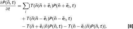On multiplying the master equation by n _i (and n _i n _j) and summing over all values of $\overrightarrow{n}$, one obtains the following equations for the moments of $P(\overrightarrow{n},t)$:

where the average of any function f is given by $\langle f\rangle \equiv {\sum }_{\overrightarrow{n}}f(\overrightarrow{n})P(\overrightarrow{n})$. Leaving aside the demographic parameters that we seek to determine, the averages on the right-hand side of the above equations can be estimated directly from the data. For example, Eq. 9 can be rewritten as $\frac{d\langle n_i\rangle }{dt}=(b_i-d_i)\langle n_i\rangle +{\sum }_j{c}_{ij}\langle n_i{n}_j\rangle$, and the averages 〈n _i〉 and 〈n _i n _j〉 are obtained by averaging the abundance data in the individual quadrats.

In total we have S + (S ² − S)/2 + S linear equations and the same number of demographic parameters. Assuming steady state, we solve the equations and find the birth, death, and interaction coefficients. One might extend our approach to determine asymmetric interaction coefficients by adding equations for higher-order moments.

For additional information, see SI Figs. S2–S5.

References

- 1.Clements FE. Carnegie Institution of Washington Publ. Vol. 242. Washington, DC: Carnegie Institution of Washington; 1916. Plant succession: Analysis of the development of vegetation. Chap 1. [Google Scholar]
- 2.Hutchinson GE. Homage to Santa Rosalia, or Why are there so many kinds of animals? Am Nat. 1958;93:145–159. [Google Scholar]
- 3.Leibold MA, McPeek MA. Coexistence of the niche and neutral perspectives in community ecology. Ecology. 2006;87:1399–1410. doi: 10.1890/0012-9658(2006)87[1399:cotnan]2.0.co;2. [DOI] [PubMed] [Google Scholar]
- 4.Leibold MA. Return of the niche. Nature. 2008;454:39–40. doi: 10.1038/454039a. [DOI] [PubMed] [Google Scholar]
- 5.Gleason HA. On the relation between species and area. Ecology. 1922;3:158–162. [Google Scholar]
- 6.MacArthur RH, Wilson EO. The Theory of Island Biogeography. Princeton: Princeton Univ Press; 1967. [Google Scholar]
- 7.Chesson P. A need for niches. Trends Ecol Evol. 1997;6:26–28. doi: 10.1016/0169-5347(91)90144-M. [DOI] [PubMed] [Google Scholar]
- 8.Hubbell SP. Princeton: Princeton Univ Press; 2001. The Unified Neutral Theory of Biodiversity and Biogeography. [DOI] [PubMed] [Google Scholar]
- 9.Volkov I, Banavar JR, Hubbell SP, Maritan A. Neutral theory and relative species abundance in ecology. Nature. 2003;424:1035–1037. doi: 10.1038/nature01883. [DOI] [PubMed] [Google Scholar]
- 10.Volkov I, Banavar JR, He F, Hubbell SP, Maritan A. Density and frequency dependence explains tree species abundance and diversity in tropical forests. Nature. 2005;438:658–661. doi: 10.1038/nature04030. [DOI] [PubMed] [Google Scholar]
- 11.Volkov I, Banavar JR, Hubbell SP, Maritan A. Patterns of relative species abundance in rainforests and coral reefs. Nature. 2007;450:45–49. doi: 10.1038/nature06197. [DOI] [PubMed] [Google Scholar]
- 12.Purvis DW, Pacala SW. Ecological drift in niche-structured communities: Neutral pattern does not imply neutral process. In: Burslem D, Pinardand MA, Hartley SE, editors. Biotic Interactions in Tropical Forests: Their Role in the Maintenance of Species Diversity. Cambridge, UK: Cambridge Univ Press; 2005. pp. 106–138. [Google Scholar]
- 13.Chave J, Muller-Landau HC, Levin SA. Comparing classical community models: Theoretical consequences for patterns of diversity. Am Nat. 2002;159:1–23. doi: 10.1086/324112. [DOI] [PubMed] [Google Scholar]
- 14.Boltzmann L. Lectures on Gas Theory. Cambridge, UK: Cambridge Univ Press; 1964. [Google Scholar]
- 15.Shannon CE. A mathematical theory of communication. Bell Syst Tech J. 1948;27:379–423. [Google Scholar]
- 16.Jaynes ET. Information theory and statistical mechanics. Phys Rev. 1957;106:620–630. [Google Scholar]
- 17.Jaynes ET. Information theory and statistical mechanics. II Phys Rev. 1957;108:171–190. [Google Scholar]
- 18.Dewar RC. Information theoretic explanation of maximum entropy production, the fluctuation theorem and self-organized criticality in non-equilibrium stationary states. J Phys A. 2003;36:631–641. [Google Scholar]
- 19.Dewar RC. Maximum entropy production and the fluctuation theorem. J Phys A. 2005;38:L371–L381. [Google Scholar]
- 20.Shipley B, Vile D, Garnier E. From plant traits to plant communities: A statistical mechanistic approach to biodiversity. Science. 2006;314:812–814. doi: 10.1126/science.1131344. [DOI] [PubMed] [Google Scholar]
- 21.Pueyo S, He F, Zillio T. The maximum entropy formalism and the idiosyncratic theory of biodiversity. Ecol Lett. 2007;10:1017–1028. doi: 10.1111/j.1461-0248.2007.01096.x. [DOI] [PMC free article] [PubMed] [Google Scholar]
- 22.Harte J, Zillio T, Conlisk E, Smith AB. Maximum entropy and the state-variable approach to macroecology. Ecology. 2008;89:2700–2711. doi: 10.1890/07-1369.1. [DOI] [PubMed] [Google Scholar]
- 23.Sibisi S, Skilling J, Brereton RG, Laue E, Staunton J. Maximum entropy signal processing in practical NMR spectroscopy. Nature. 1984;311:446–447. [Google Scholar]
- 24.Kitaura R, et al. Formation of a one-dimensional array of oxygen in a microporous metal-organic solid. Science. 2002;298:2358–2361. doi: 10.1126/science.1078481. [DOI] [PubMed] [Google Scholar]
- 25.Schneidman E, Berry MJ, Segev R, Bialek W. Weak pairwise correlations imply strongly correlated network states in a neural population. Nature. 2006;440:1007–1012. doi: 10.1038/nature04701. [DOI] [PMC free article] [PubMed] [Google Scholar]
- 26.Lezon T, Banavar JR, Cieplak M, Maritan A, Fedoroff NV. Using entropy maximization to infer genetic interaction networks from gene expression patterns. Proc Natl Acad Sci USA. 2006;103:19033–19038. doi: 10.1073/pnas.0609152103. [DOI] [PMC free article] [PubMed] [Google Scholar]
- 27.Pielou EC. An Introduction to Mathematical Ecology. New York: Wiley; 1969. [Google Scholar]
- 28.Azaele S, Pigolotti S, Banavar JR, Maritan A. Dynamical evolution of ecosystems. Nature. 2006;444:926–928. doi: 10.1038/nature05320. [DOI] [PubMed] [Google Scholar]
- 29.Preparata FR, Shamos MI. Computational Geometry: An Introduction. New York: Springer; 2004. [Google Scholar]
- 30.McKane AJ, Newman TJ. Stochastic models in population biology and their deterministic analogs. Phys Rev E. 2004;70:041902. doi: 10.1103/PhysRevE.70.041902. [DOI] [PubMed] [Google Scholar]
- 31.Brown JH, Bedrick EJ, Ernest SKM, Cartron JLE, Kelly JF. Constraints on negative relationships: Mathematical causes and ecological consequences. In: Taper ML, Lele S, Lewin-Koh N, editors. The Nature of Scientific Evidence. Baltimore: Johns Hopkins Univ Press; 2004. [Google Scholar]
- 32.Van Kampen NG. Stochastic Processes in Physics and Chemistry. Amsterdam: North-Holland; 2001. [Google Scholar]
Associated Data
This section collects any data citations, data availability statements, or supplementary materials included in this article.