Abstract
In a practical classifier design problem, the sample size is limited, and the available finite sample needs to be used both to design a classifier and to predict the classifier’s performance for the true population. Since a larger sample is more representative of the population, it is advantageous to design the classifier with all the available cases, and to use a resampling technique for performance prediction. We conducted a Monte-Carlo simulation study to compare the ability of different resampling techniques in predicting the performance of a neural network (NN) classifier designed with the available sample. We used the area under the receiver operating characteristic curve as the performance index for the NN classifier. We investigated resampling techniques based on the cross-validation, the leave-one-out method, and three different types of bootstrapping, namely, the ordinary, .632, and .632+ bootstrap. Our results indicated that, under the study conditions, there can be a large difference in the accuracy of the prediction obtained from different resampling methods, especially when the feature space dimensionality is relatively large and the sample size is small. Although this investigation is performed under some specific conditions, it reveals important trends for the problem of classifier performance prediction under the constraint of a limited data set.
1. Introduction
Classification of a set of vectors into two classes is a common application for neural networks (NNs). In practice, the NN classifier is designed using a finite training set, which may not fully represent the true distribution of the two classes in the general population. Finite training sample size presents two problems. First, one has to pay a penalty for the finite sample size, i.e., the classifier is less accurate than one that would be trained using the true distributions. Second, if one is also required to make a prediction of the accuracy of the designed classifier, one has to use the finite sample not only to train the classifier, but also to predict its performance for the true population. The goal of this study is to investigate the bias and error of this prediction for several resampling techniques.
We are particularly motivated by applications in computer-aided diagnosis (CAD), which aims at designing automated image analysis systems to aid radiologists in detecting and characterizing lesions on medical images. In most medical applications, one has only a relatively small population of patient samples with ground truth available for training the CAD system. An intuitive approach would be to use all the available cases for classifier design, with the expectation that using as many cases as possible potentially maximizes the accuracy of the designed classifier. However, the CAD developer will also typically be required to predict the performance that can be expected from the designed classifier. Since all cases have been used for classifier design, one has to use a resampling technique to estimate the performance of the designed classifier when it is applied to the true population.
Classifier performance estimation has previously been addressed in many contexts. In the context of CAD, a commonly used performance measure is the area under the receiver operating characteristics (ROC) curve, referred to as AUC below. To our knowledge, only very preliminary studies have been conducted to investigate the problem of AUC prediction for a classifier under the constraint of a limited data set, and mostly for linear classifiers (Sahiner et al., 2001; Yousef, Wagner, & Loew, 2004). In a previous study, we investigated the performance of different resampling methods for a backpropagation NN using Monte Carlo simulation under a number of conditions for the number of available samples from each class feature space dimensionality, and a limited set of feature space distributions (Sahiner, Chan, & Hadjiiski, 2007). The current study extends this previous work by including additional conditions for class distributions and class separability.
2. Methods
Five resampling methods were compared, including three variations of the bootstrap method, namely, the ordinary, .632 and .632+ bootstrap, and the Fukunaga-Hayes (F-H) and the leave-one-out (LOO) methods.
A. The Ordinary Bootstrap
Let F represent the true distribution of the data, and let x = (x1, x2,…, xN) be the available sample of size N, where the boldface letter x denotes a set of cases (i.e., a sample), and the italic letter x denotes a data vector (i.e., a case). In bootstrap, an empirical discrete distribution F̂ is defined such that a probability of 1/N is assigned to each case xi, A bootstrap sample, denoted as x*= (x1*, x2*,…, xN*), of size N is then randomly drawn with replacement from x, which is equivalent to random drawing from the empirical distribution F̂. In classifier performance evaluation, the bootstrap method generally involves the estimation of the bias of the resubstitution method, and the removal of this bias from the resubstitution performance to obtain an estimate of the true performance (Efron, 1983). Application to the estimation of the test AUC is described below.
Let AUC(Strain,Stest) denote the test AUC value, obtained when the classifier trained on the set Strain is applied to the test set Stest. Let w denote the bias of the resubstitution method. Using the bootstrap technique, one generates B bootstrap samples, x*1,x*2,…,x*B, where each sample x*b = (x1*b, x2*b, …, xN*b) is obtained by randomly drawing N data vectors (with replacement) from the original data set x. In the ordinary bootstrap method, the bias of the resubstitution method is estimated from the bootstrap sample x*b as
| (1) |
This difference, averaged over B bootstrap samples, provides an estimate for the bias of the resubstitution method:
| (2) |
This estimate is then subtracted from the true resubstitution AUC value, obtained by training and testing on the set of all available data, to correct for the bias
| (3) |
B. The .632 Bootstrap
Let x*b (0) denote the subset of data vectors in x that do not appear in x*b for the bth bootstrap. A possibility is to consider AUC(x*b, x*b (0)) as the classifier performance estimate. Using a probabilistic argument, Efron demonstrates that AUC(x*b, x*b (0)) is pessimistically biased, because x*b (0) are farther away from x than a typical test sample randomly drawn from the true population (Efron, 1983). On the average, the ratio of the distances from these two groups to x is 1/(1 − e−1) = 1/0.632. The bias of the resubstitution method can therefore be estimated from the bootstrap sample x*b as
| (4) |
The estimate for the bias of the .632 method, ŵ.632, is found by averaging Eq. (4) over B bootstrap samples. The AUC value estimated from the .632 method is then given by
| (5) |
C. The .632+ Bootstrap
The .632+ estimator was designed by Efron to address the issue of the bias of the .632 estimator (Efron & Tibshirani, 1997). Starting with the example of a classification problem in which the data is useless (AUC=0.5), Efron shows that for overtrained classifiers, the .632 estimator for the classifier performance can be optimistically biased. The original definition of the .632+ estimator can be found in the literature. In this study, the AUC value estimated from the .632+ method is defined as
| (6) |
where
| (7) |
| (8) |
and
| (9) |
Notice that the .632 estimate (Eq. (5)) can be thought of as a special case of the .632+ estimate with α = 0.632 and AUC′ (x*b, x*b (0)) = AUC(x*b,x*b (0)). This definition is slightly different from that used in (Efron & Tibshirani, 1997) in that the relative overfitting rate R and the weight α are calculated for each bootstrap replication. Also, the definition (9) for the overfitting rate contains an additional condition related to whether AUC(x*b, x*b (0)) is smaller than the chance (no-information) AUC value of 0.5, which was not included in (Efron & Tibshirani, 1997).
D. The Fukunaga-Hayes Method
Another method to estimate the performance of a classifier that can be designed with N cases is to partition them into a training group of Ntrain cases and a test group of Ntest = N − Ntrain cases. One can repeat the partitioning process P times, and use the average test AUC as the performance estimate. A disadvantage of this method is that since Ntrain < N, the designed classifier may have a lower performance than the one that would have been trained with N cases. Fukunaga and Hayes studied the dependence of the classifier performance on the training sample size Ntrain, and showed that under a wide range of conditions, the probability of misclassification (PMC) error varies linearly with 1/Ntrain (K Fukunaga & Hayes, 1989). Based on this observation, they suggested that one can vary Ntrain < N in a range of values, obtain a linear regression to the PMC, and then extrapolate to find the PMC for Ntrain ≥ N. In our previous work, we applied this method for performance estimation using the AUC. For various classifiers and Gaussian class distributions, it was observed that the dependence of the AUC value can be closely approximated by a linear relationship in a sample size range where higher-order terms 1/Ntrain can be neglected (Chan, Sahiner, Wagner, & Petrick, 1999). The implementation in the current study uses four values for Ntrain < N for finding the linear regression, and P training-test partitioning sets at each of these values to obtain the F-H prediction of the classification performance, , at Ntrain = N.
E. The Leave-One-Out Method
In the LOO technique, one designs N classifiers using the sample x= (x1, x2, …, xN). In the design of the ith classifier, all cases are used except case xi, which is reserved as a test case. Since each classifier is designed using N−1 cases, the number of trainers is very close to the number of available cases. In our application, we accumulated all N test results in an array and computed for the LOO method.
F. Summary Measures of Prediction Accuracy
As discussed in the Introduction, our goal is to predict the performance of the classifier trained with the given set of N cases when it is applied to the true population. The true performance is therefore AUC(x, F), which is referred to as the true conditional performance below because it is conditional on the available training set x. Several different class distributions F were simulated, as discussed below. We define one experiment j as the selection of a sample x from F. The true conditional performance for the jth experiment (conditioned on the available training set), AUCj (x, F), is obtained by training the classifier with x, drawing an additional random test sample of 2,000 cases from the distribution of each class, and testing the designed classifier with this data set of 4,000 test cases. The number of test cases, 4,000, is chosen to be large enough so that the distribution of the test data is close to F. The AUC is calculated using the LABROC program (Metz, Herman, & Shen, 1998), which uses a maximum likelihood estimation algorithm to fit a binormal ROC curve to the classifier output after proper binning. Note that the true conditional performance AUCj (x, F) depends on x, and therefore changes in each experiment. The prediction error of a resampling method for the jth experiment was then defined as
| (10) |
where r stands for one of the five different sampling methods, i.e., the ordinary bootstrap, .632 bootstrap, .632+ bootstrap, F-H, or LOO, and denotes the predicted AUC for experiment j using the resampling method r. For each condition discussed below, we performed J=200 experiments. The bias of the resampling technique was defined as the average of Ej,r over J experiments.
To quantify how close the predicted and true conditional performances are, we used the root-mean-squared error (RMSE)
| (11) |
The mean and the standard deviation of the predicted accuracy were also estimated:
| (12) |
| (13) |
G. Feature Spaces and Sample Sizes
We investigated two categories of class distributions. Class distributions in the first category were assumed to follow multivariate normal distributions with equal covariance matrices. It has been shown in the literature (K. Fukunaga, 1990) that the covariance matrices can be simultaneously diagonalized without affecting the analysis. We therefore used an identity matrix for the covariance of both classes. We assumed that the mean difference between the two classes was equal for each feature. The value of the difference was chosen such that the AUC of the classifier designed and tested with infinite sample size would be approximately 0.8. The dimensionality of the feature space, k, was varied from 3 to 15.
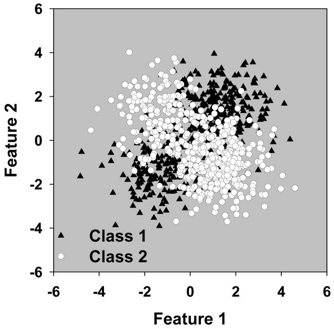
Class distributions in the second category were assumed to be a mixture of overlapping Gaussian distributions. The dimensionality of the feature space, k, was varied from 2 to 8. Figure 1 shows an example scatter plot of the class distributions for k = 2. Each class was a mixture of two Gaussians where each Gaussian had identity covariance matrix. The mean vectors the two Gaussians for class 1 were [M, M] and [−M, −M] respectively, while those for class 2 were [M, −M] and [−M, M] respectively. For k ≥ 3, the means of the Gaussians in the first two dimensions were ±M, and those in the remaining dimensions were all zero, so that the separability of the two classes was the same for different values of k. The separability of the two classes was varied by changing M. For each k, we performed experiments with three different values of M. The AUC of the classifier designed and tested with an infinite sample size with these three different values are approximately 0.95, 0.89, and 0.79. These are referred to as the high, medium-high, and medium separability conditions below, respectively.
Fig. 1.
An example scatter plot of the class distributions from the second category.
The number of cases from class 1 and class 2, denoted by n1 and n2, were assumed to be equal so that n1 = n2 = N/2. The total number of cases in the sample N was varied between 50 and 120.
H. The NN Classifier
Many different NN architectures and training methods can be used for a classification task. In this study, we used a three-layered NN trained with a back-propagation method. The NN had k input nodes, h hidden nodes, one output node, and the architecture is denoted as k − h − 1. The nodes were fully connected, and the weights were trained using a minimum sum-of-squares-error criterion. Since our purpose was not to optimize the NN architecture, but to test different resampling schemes to predict the accuracy of an NN that would be trained with the given sample of size N, we did not perform an exhaustive search to determine how many nodes in the hidden layer and what kind of stopping criterion maximized the AUC. However, if the selected NN parameters result in a classifier having a performance that is far from the optimal, the simulation results would be irrelevant in practice. To ensure that this did not happen, we first trained different NNs with a sample size varying between 50 and 120 while the number of hidden nodes and the number of training iterations were varied. The trained NNs were tested with a very large sample size. Using the resulting test Az values, we chose a k-3-1 architecture for class distributions in the first category (Gaussian) and a k-5-1 architecture for class distributions in the second category (mixture of Gaussians). For the first category, the number of training iterations were 750, 400 and 100 for k=3, 9, and 15, respectively. For the second category, the number of training iterations were 1000, 900, and 800 for k=2, 5, and 8, respectively.
3. Results
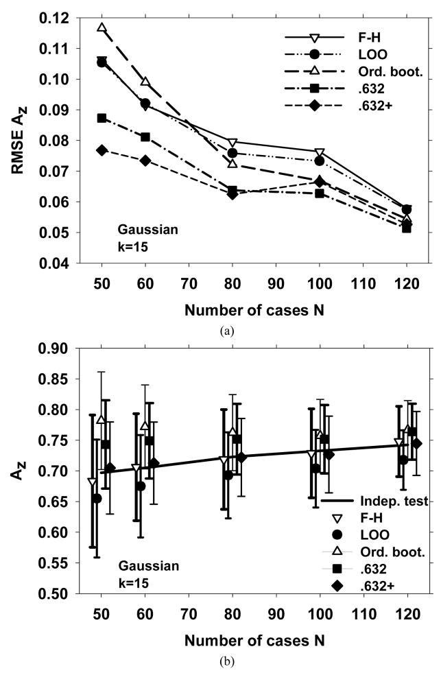
Figure 2 shows the results obtained with the five different resampling methods and five sample sizes (N=50, 60, 80, 100, and 120) for Gaussian class distributions and k=15. The RMSE, and the average performance were plotted in Figures 2(a) and 2(b), respectively. Fig. 2(b) shows that the F-H method has a low bias for this condition. However, the .632 and .632+ bootstrap methods perform better than the F-H in terms of the RMSE (Fig. 2(a))..
Fig. 2.
Simulation results for a 15-dimensional Gaussian feature space (a) The root-mean-squared-error (RMSE) of the AUC estimated with the five resampling techniques. (b) The mean of the AUC and ±(standard deviation), shown as error bars. The solid line is the average of the true conditional AUC, the standard deviation of which is not shown for the clarity of the figure. The data points are plotted slightly offset, centered around a given value of N to prevent the marks and error bars from overlapping with each other.
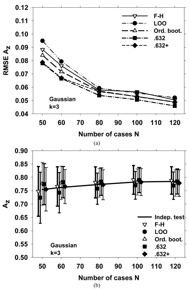
The simulation conditions in Fig. 3 are similar to those in Fig. 2, except that the feature space dimensionality was reduced to three. The differences in the bias for the different resampling schemes are smaller and the RMSE errors are closer to each other for k=3 compared to k=15, although the .632 and .632+ bootstrap methods still have a small advantage over the others for small N.
Fig. 3.
Simulation results for a 3-dimensional Gaussian feature space (a) The RMSE of the AUC, and (b) The mean of the AUC and ±(standard deviation), shown as error bars.
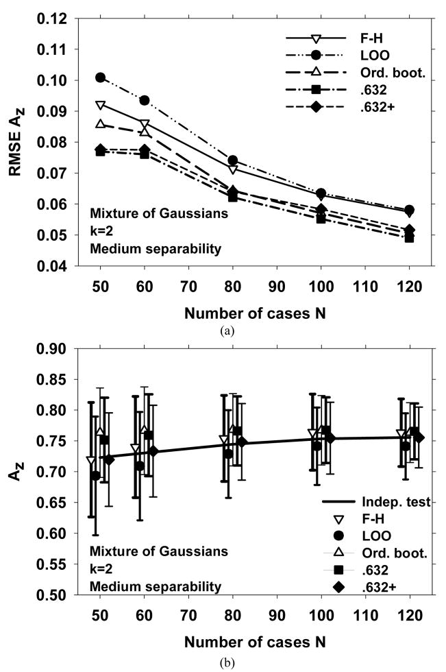
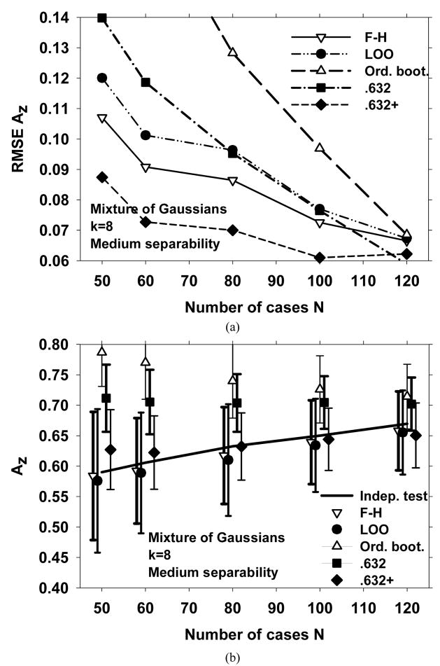
Figures 4 and 5 show the simulation results for a mixture of Gaussians with medium separability, and with k=2 and 8, respectively. The trends in Fig. 4 are similar to those for Fig. 3. At small sample sizes, the average AUC estimated by F-H and .632+ methods are closest to independent testing. The .632 and .632+ methods have the smallest RMSE. However, Fig. 5 shows that when the dimensionality of the feature space is larger, the average AUC estimated by the .632+ method at small sample sizes is no longer unbiased, whereas the bias of the F-H method is still close to zero. The .632 method has a large bias, and as a result, has a higher RMSE than LOO and F-H methods (Fig. 5(b)).
Fig. 4.
Simulation results for a 2-dimensional feature space of mixture of Gaussians with medium separability. (a) The RMSE of the AUC, and (b) The mean of the AUC and ±(standard deviation), shown as error bars.
Fig. 5.
Simulation results for an 8-dimensional feature space of mixture of Gaussians with medium separability. (a) The RMSE of the AUC, and (b) The mean of the AUC and ±(standard deviation), shown as error bars.
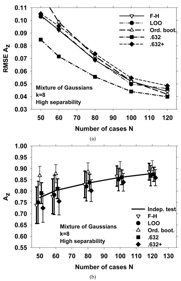
Figure 6 shows the simulation results for a mixture of Gaussians with k=8, and high separability. In contrast to the other conditions discussed above, the .632+ method has the largest RMSE for sample sizes between 80 and 120 under this condition. This is partly explained by observing that the .632+ method has a relatively large negative bias. On the other hand, the .632 method, which had a positive bias for other simulation conditions, seems almost unbiased under this condition, and has the lowest RMSE.
Fig. 6.
Simulation results for an 8-dimensional feature space of mixture of Gaussians with high separability. (a) The RMSE of the AUC, and (b) The mean of the AUC and ±(standard deviation), shown as error bars.
The average true conditional AUC, and the bias, standard deviation, and root-mean-squared error obtained over 250 experiments for different resampling methods and different conditions for the simulated data sets are summarized in Table 1.
Table 1.
The average true conditional AUC, and the bias, standard deviation, and root-mean-squared error obtained over 250 experiments for different resampling methods for each condition A–H. N denotes the total number of training samples drawn in each experiment. The legend for the first column is: G: Gaussian data, MG: Mixture of Gaussian data;
3: 3-dimensional, f15: 15 dimensional, f2: 2-dimensional, f8: 8-dimensional data;
M: Medium separability, MH: Medium-high separability, H: High separability between the two classes.
| N | True AUC |
Fukunaga-Hayes | Leave-one-out | Ordinary bootstrap | .632 bootstrap | .632+ bootstrap | |||||||||||
|---|---|---|---|---|---|---|---|---|---|---|---|---|---|---|---|---|---|
| Bias | Std | RMSE | Bias | Std | RMSE | Bias | Std | RMSE | Bias | Std | RMSE | Bias | Std | RMSE | |||
| A | 50 | 0.754 | −0.007 | 0.093 | 0.088 | −0.031 | 0.096 | 0.095 | 0.022 | 0.080 | 0.084 | 0.020 | 0.077 | 0.078 | 0.001 | 0.081 | 0.079 |
| G | 60 | 0.762 | 0.004 | 0.074 | 0.076 | −0.020 | 0.076 | 0.079 | 0.017 | 0.063 | 0.072 | 0.020 | 0.059 | 0.066 | 0.003 | 0.064 | 0.067 |
| f3 | 80 | 0.774 | 0.008 | 0.058 | 0.058 | −0.016 | 0.059 | 0.059 | 0.007 | 0.054 | 0.057 | 0.010 | 0.051 | 0.054 | −0.001 | 0.056 | 0.057 |
| 100 | 0.783 | 0.008 | 0.054 | 0.057 | −0.013 | 0.052 | 0.056 | 0.000 | 0.049 | 0.053 | 0.007 | 0.047 | 0.051 | −0.001 | 0.051 | 0.053 | |
| 120 | 0.785 | 0.004 | 0.051 | 0.050 | −0.016 | 0.051 | 0.052 | −0.006 | 0.049 | 0.049 | 0.000 | 0.047 | 0.046 | −0.006 | 0.050 | 0.049 | |
|
| |||||||||||||||||
| B | 50 | 0.697 | −0.014 | 0.108 | 0.106 | −0.042 | 0.096 | 0.105 | 0.085 | 0.080 | 0.117 | 0.046 | 0.072 | 0.087 | 0.008 | 0.075 | 0.077 |
| G | 60 | 0.705 | 0.001 | 0.087 | 0.091 | −0.030 | 0.083 | 0.092 | 0.067 | 0.068 | 0.099 | 0.044 | 0.061 | 0.081 | 0.007 | 0.067 | 0.073 |
| f15 | 80 | 0.723 | −0.004 | 0.081 | 0.080 | −0.030 | 0.070 | 0.076 | 0.040 | 0.062 | 0.072 | 0.029 | 0.057 | 0.064 | −0.001 | 0.063 | 0.062 |
| 100 | 0.733 | −0.004 | 0.073 | 0.076 | −0.029 | 0.063 | 0.073 | 0.024 | 0.060 | 0.067 | 0.019 | 0.056 | 0.063 | −0.006 | 0.063 | 0.066 | |
| 120 | 0.742 | 0.005 | 0.057 | 0.058 | −0.025 | 0.049 | 0.057 | 0.024 | 0.048 | 0.054 | 0.021 | 0.046 | 0.051 | 0.002 | 0.052 | 0.053 | |
|
| |||||||||||||||||
| C | 50 | 0.723 | −0.003 | 0.093 | 0.092 | −0.030 | 0.096 | 0.101 | 0.040 | 0.073 | 0.086 | 0.028 | 0.069 | 0.077 | −0.004 | 0.076 | 0.078 |
| MG | 60 | 0.730 | 0.010 | 0.082 | 0.086 | −0.021 | 0.088 | 0.093 | 0.036 | 0.071 | 0.083 | 0.029 | 0.067 | 0.076 | 0.003 | 0.074 | 0.078 |
| f2 | 80 | 0.745 | 0.010 | 0.070 | 0.071 | −0.016 | 0.071 | 0.074 | 0.024 | 0.059 | 0.064 | 0.022 | 0.056 | 0.062 | 0.004 | 0.062 | 0.064 |
| M | 100 | 0.753 | 0.011 | 0.062 | 0.063 | −0.012 | 0.063 | 0.063 | 0.014 | 0.056 | 0.057 | 0.014 | 0.053 | 0.055 | 0.001 | 0.058 | 0.058 |
| 120 | 0.756 | 0.008 | 0.055 | 0.057 | −0.015 | 0.054 | 0.058 | 0.008 | 0.049 | 0.050 | 0.010 | 0.045 | 0.049 | 0.000 | 0.049 | 0.052 | |
|
| |||||||||||||||||
| D | 50 | 0.590 | −0.006 | 0.105 | 0.107 | −0.014 | 0.118 | 0.120 | 0.197 | 0.056 | 0.208 | 0.121 | 0.055 | 0.140 | 0.037 | 0.066 | 0.087 |
| MG | 60 | 0.606 | −0.014 | 0.087 | 0.091 | −0.017 | 0.099 | 0.101 | 0.164 | 0.060 | 0.178 | 0.099 | 0.053 | 0.119 | 0.017 | 0.060 | 0.073 |
| f8 | 80 | 0.633 | −0.015 | 0.080 | 0.086 | −0.023 | 0.092 | 0.096 | 0.107 | 0.061 | 0.128 | 0.071 | 0.047 | 0.095 | 0.000 | 0.055 | 0.070 |
| M | 100 | 0.650 | −0.011 | 0.069 | 0.073 | −0.016 | 0.077 | 0.077 | 0.076 | 0.055 | 0.097 | 0.054 | 0.043 | 0.076 | −0.006 | 0.051 | 0.061 |
| 120 | 0.670 | −0.012 | 0.065 | 0.067 | −0.015 | 0.069 | 0.067 | 0.045 | 0.053 | 0.069 | 0.032 | 0.044 | 0.059 | −0.019 | 0.053 | 0.062 | |
|
| |||||||||||||||||
| E | 50 | 0.844 | −0.009 | 0.061 | 0.066 | −0.022 | 0.072 | 0.079 | 0.026 | 0.055 | 0.066 | 0.013 | 0.053 | 0.060 | −0.005 | 0.061 | 0.066 |
| MG | 60 | 0.850 | 0.001 | 0.058 | 0.062 | −0.014 | 0.065 | 0.069 | 0.024 | 0.053 | 0.062 | 0.013 | 0.051 | 0.057 | 0.000 | 0.058 | 0.061 |
| f2 | 80 | 0.862 | 0.005 | 0.047 | 0.050 | −0.008 | 0.049 | 0.052 | 0.016 | 0.042 | 0.048 | 0.011 | 0.040 | 0.046 | 0.003 | 0.044 | 0.048 |
| MH | 100 | 0.869 | 0.006 | 0.041 | 0.042 | −0.009 | 0.041 | 0.043 | 0.010 | 0.038 | 0.039 | 0.006 | 0.036 | 0.037 | 0.001 | 0.038 | 0.039 |
| 120 | 0.873 | 0.001 | 0.037 | 0.039 | −0.014 | 0.036 | 0.041 | 0.001 | 0.034 | 0.036 | 0.000 | 0.032 | 0.035 | −0.004 | 0.034 | 0.036 | |
|
| |||||||||||||||||
| F | 50 | 0.685 | −0.025 | 0.095 | 0.110 | −0.023 | 0.105 | 0.116 | 0.148 | 0.046 | 0.164 | 0.068 | 0.050 | 0.104 | −0.011 | 0.067 | 0.093 |
| MG | 60 | 0.709 | −0.021 | 0.086 | 0.097 | −0.020 | 0.099 | 0.101 | 0.118 | 0.052 | 0.137 | 0.048 | 0.049 | 0.089 | −0.024 | 0.064 | 0.089 |
| f8 | 80 | 0.746 | −0.012 | 0.076 | 0.085 | −0.013 | 0.078 | 0.082 | 0.073 | 0.054 | 0.098 | 0.027 | 0.044 | 0.071 | −0.029 | 0.056 | 0.081 |
| MH | 100 | 0.777 | −0.004 | 0.060 | 0.065 | −0.013 | 0.064 | 0.063 | 0.046 | 0.047 | 0.067 | 0.014 | 0.039 | 0.052 | −0.026 | 0.049 | 0.064 |
| 120 | 0.799 | 0.000 | 0.053 | 0.058 | −0.014 | 0.059 | 0.059 | 0.025 | 0.047 | 0.053 | 0.003 | 0.040 | 0.049 | −0.027 | 0.049 | 0.064 | |
|
| |||||||||||||||||
| G | 50 | 0.911 | −0.018 | 0.044 | 0.055 | −0.016 | 0.051 | 0.060 | 0.021 | 0.036 | 0.049 | 0.005 | 0.036 | 0.045 | −0.005 | 0.041 | 0.049 |
| MG | 60 | 0.919 | −0.011 | 0.037 | 0.042 | −0.013 | 0.048 | 0.053 | 0.016 | 0.035 | 0.043 | 0.003 | 0.035 | 0.040 | −0.004 | 0.039 | 0.044 |
| f2 | 80 | 0.926 | −0.001 | 0.029 | 0.032 | −0.005 | 0.032 | 0.037 | 0.013 | 0.027 | 0.034 | 0.006 | 0.026 | 0.032 | 0.002 | 0.028 | 0.034 |
|
| |||||||||||||||||
| H | 100 | 0.933 | −0.001 | 0.026 | 0.028 | −0.008 | 0.029 | 0.031 | 0.006 | 0.025 | 0.027 | 0.002 | 0.024 | 0.026 | −0.001 | 0.025 | 0.027 |
| 120 | 0.935 | −0.003 | 0.023 | 0.024 | −0.010 | 0.024 | 0.028 | 0.001 | 0.022 | 0.024 | −0.002 | 0.021 | 0.023 | −0.004 | 0.022 | 0.024 | |
| H | 50 | 0.771 | −0.034 | 0.081 | 0.104 | −0.021 | 0.094 | 0.103 | 0.097 | 0.042 | 0.121 | 0.020 | 0.046 | 0.085 | −0.046 | 0.063 | 0.105 |
| MG | 60 | 0.803 | −0.026 | 0.077 | 0.092 | −0.020 | 0.087 | 0.093 | 0.074 | 0.040 | 0.099 | 0.008 | 0.044 | 0.072 | −0.048 | 0.060 | 0.096 |
| f8 | 80 | 0.836 | −0.006 | 0.059 | 0.069 | −0.015 | 0.064 | 0.069 | 0.050 | 0.039 | 0.072 | 0.002 | 0.037 | 0.056 | −0.034 | 0.048 | 0.074 |
| H | 100 | 0.861 | 0.005 | 0.045 | 0.052 | −0.010 | 0.050 | 0.050 | 0.032 | 0.038 | 0.052 | 0.000 | 0.033 | 0.044 | −0.022 | 0.040 | 0.055 |
| 120 | 0.878 | 0.008 | 0.037 | 0.044 | −0.010 | 0.045 | 0.046 | 0.020 | 0.037 | 0.042 | −0.004 | 0.031 | 0.040 | −0.019 | 0.036 | 0.048 | |
4. Discussion and conclusion
In many applications, one has only a finite sample size to design a classifier and to assess its performance. Since a larger sample is more representative of the population, it is advantageous to design the classifier with all the available cases, and then to assess the accuracy of the designed classifier using a resampling technique. In this study, we compared the performances of five such resampling techniques for backpropagation NN classifiers, using the AUC as the performance index.
The bias of the resampling method is important because the use of a method that consistently provides optimistic estimates may be misleading about the potential of a classification technique, especially in CAD. The ordinary bootstrap method had a relatively large optimistic bias for all the conditions in this study, and we believe that in the form that was used in this investigation, is not suitable for classifier performance estimation. The F-H method had the smallest overall bias among the methods studied, followed by the 0.632+ method (Table 1). However, depending on the feature space distribution and dimensionality, some of these trends may be reversed. For example, for the 8-dimensional mixture of Gaussians with high separability, the 0.632 and LOO methods had lower bias than F-H and 0.632+ at low training sample size (Fig. 6(b)).
The magnitude of the error in performance estimation, measured by the RMSE in this study, may be more important than the bias in many situations. A smaller error magnitude for a resampling method means that, for a given sample, one has a higher chance to get an estimate that is closer to the truth. For the class distributions considered in this study, the difference in the RMSE obtained using different resampling methods can be large, especially when the feature space dimensionality is large and the number of available samples is small. Under most of the conditions studied, the .632 and .632+ bootstrap methods had either lower or similar RMSE compared to other resampling methods. An exception to this was the 8-dimensional mixture of Gaussians with medium separability, for which the .632 technique had considerably higher RMSE than LOO and F-H (Fig. 5(a)).
Both the bias and standard deviation of the resampling method contribute to the RMSE. The relatively large, optimistic bias of the .632 technique for the 8-dimensional mixture of Gaussians with medium separability (Fig. 5(b)) may be the major reason why this technique had higher RMSE than LOO and F-H in Fig. 5(a). However, under most of the other conditions, the standard deviation of the resampling technique may have been the major contributor to the RMSE. When this is the case, one may expect the.632 and .632+ methods to outperform LOO and F-H because, by design, the bootstrap methods have a smaller standard deviation.
The .632+ method was designed primarily to reduce the optimistic bias of the .632 method. Our simulation study indicates that this goal was met particularly well when the two classes were not well-separated in the feature space. However, when the two classes had high or medium-high separation, the .632+ method may result in an over-correction of the .632 method, and provide a pessimistic bias (Fig. 6(b) and conditions F and H in Table 1).
The method used for finding the .632+ AUC estimate in this study is different from that used in (Efron & Tibshirani, 1997) for finding the error rate, and the equations are different from those used in (Yousef, Wagner, & Loew, 2004) and (Efron & Tibshirani, 1997) for AUC, in two aspects. First, our method performs the nonlinear operation given by (9) for each bootstrap replication, whereas (Yousef, Wagner, & Loew, 2004) and (Efron & Tibshirani, 1997) perform an average over all bootstrap replications before applying the nonlinearity. Our experiments with the latter method (not shown) indicated that the difference in the two methods did not result in a major difference in the .632+ AUC estimate. The second difference in our 632+ AUC estimate was the additional condition in (9) related to whether AUC(x*b, x*b (0)) is smaller than the chance (no-information) AUC value of 0.5. Our experiments indicated that without this condition in (9), our .632+ AUC estimate for the medium separability condition may have a larger positive bias. Note that without this condition, the overfitting rate R will have a large discontinuity when it is plotted as a function of AUC(x*b, x*b (0)).
The understanding of bias, variance, and RMSE issues in classifier performance estimation will provide us a useful guide to reduce errors in the assessment of classifier performance.
Acknowledgments
This work was supported in part by the USPHS under grants CA095153 and CA118305. The authors are grateful to Charles E. Metz, Ph.D., for the LABROC program.
Footnotes
Publisher's Disclaimer: This is a PDF file of an unedited manuscript that has been accepted for publication. As a service to our customers we are providing this early version of the manuscript. The manuscript will undergo copyediting, typesetting, and review of the resulting proof before it is published in its final citable form. Please note that during the production process errors may be discovered which could affect the content, and all legal disclaimers that apply to the journal pertain.
References
- Chan HP, Sahiner B, Wagner RF, Petrick N. Classifier design for computer-aided diagnosis: Effects of finite sample size on the mean performance of classical and neural network classifiers. Medical Physics. 1999;26:2654–2668. doi: 10.1118/1.598805. [DOI] [PubMed] [Google Scholar]
- Efron B. Estimating the error rate of a prediction rule: Improvement on cross-validation. Journal of the American Statistical Association. 1983;78:316–331. [Google Scholar]
- Efron B, Tibshirani R. Improvements on cross-validation: The .632+ bootstrap method. Journal of the American Statistical Association. 1997;92:548–560. [Google Scholar]
- Fukunaga K. Introduction to Statistical Pattern Recognition. 2. New York: Academic Press; 1990. [Google Scholar]
- Fukunaga K, Hayes RR. Effects of sample size on classifier design. IEEE Transactions on Pattern Analysis and Machine Intelligence. 1989;11:873–885. [Google Scholar]
- Metz CE, Herman BA, Shen JH. Maximum-likelihood estimation of receiver operating characteristic (ROC) curves from continuously-distributed data. Statistics in Medicine. 1998;17:1033–1053. doi: 10.1002/(sici)1097-0258(19980515)17:9<1033::aid-sim784>3.0.co;2-z. [DOI] [PubMed] [Google Scholar]
- Sahiner B, Chan HP, Hadjiiski L. Classifier performance estimation under the constraint of a finite sample size: Resampling schemes applied to neural network classifiers. Proc. 2007 International Joint Conference on Neural Networks; 2007. pp. 1762–1766. [DOI] [PMC free article] [PubMed] [Google Scholar]
- Sahiner B, Chan HP, Petrick N, Hadjiiski LM, Paquerault S, Gurcan MN. Resampling schemes for estimating the accuracy of a classifier designed with a limited data set. Presented at the Medical Image Perception Conference IX, Airlie Conference Center; Warrenton, VA. 2001. [Google Scholar]
- Yousef WA, Wagner RF, Loew MH. Comparison of non-parametric methods for assessing classifier performance in terms of ROC parameters. Applied Imagery Pattern Recognition Workshop, 33rd; IEEE Computer Society; 2004. pp. 190–195. [Google Scholar]


