A Comparison of Three Perturbation Molecular Dynamics Methods for Modeling Conformational Transitions

Abstract

Targeted, steered, and biased molecular dynamics (MD) are widely used methods for studying transition processes of biomolecules. They share the common feature of adding external perturbations along a conformational progress variable to guide the transition in a predefined direction in conformational space, yet differ in how these perturbations are applied. In the present paper, we report a comparison of these three methods on generating transition paths for two different processes: the unfolding of the B domain of protein A and a conformational transition of the catalytic domain of a Src kinase Lyn. Transition pathways were calculated with different simulation parameters including the choice of progress variable and the simulation length or biasing force constant. A comparison of the generated paths based on structural similarity finds that the three perturbation MD methods generate similar transition paths for a given progress variable in most cases. On the other hand, the path depends more strongly on the choice of progress variable used to move the system between the initial and final states. Potentials of mean force (PMF) were calculated starting from unfolding trajectories to estimate the relative probabilities of the paths. A lower PMF was found for the lowest biasing force constant with BMD.

1 Introduction

Functionally important dynamic processes of proteins, such as folding/unfolding and allosteric conformational transitions, occur on the µs-ms timescale. Molecular dynamics simulation is a useful tool to elucidate the atomistic detail of protein dynamics, however, simulations of all-atom models are limited to the sub-µsec time range. To overcome this timescale problem, methods that utilize the principles of molecular dynamics, with some external perturbations to accelerate the reaction and guide the system toward a target state, have been developed. ^1–6 Here, such methods are collected under the title of “perturbation molecular dynamics”. They aim to identify possible transition pathways as well as energy barriers and metastable intermediates. Such pathways can then be further examined by thermodynamic simulation methods.

The most commonly used perturbation molecular dynamics methods are targeted molecular dynamics (TMD), steered molecular dynamics (SMD) and biased molecular dynamics (BMD). These methods share the common feature of guiding the transition between two end-states through some progress variable (reaction coordinate) though they differ in the way that the progress variable is controlled. As originally introduced by Schlitter, ^1,2 the TMD methodology imposes a time-dependent holonomic constraint on the RMSD to a target structure. SMD simulations were first used by Grubmueller³ and Leech,⁴ and were widely applied shortly after by Schulten et al. ^7–10 SMD is akin to AFM in that a harmonic restraint based on a reference point moves the system toward the target when the reference point is updated. We note that in some later publications ^11–16 the term TMD was associated with the RMSD progress variable with harmonic restraint rather than holonomic constraint. In the present paper, we denote the holonomic constraint as TMD and the harmonic restraint as SMD to distinguish the perturbation form regardless of the progress variable. BMD, also known as the adiabatic bias molecular dynamics, was originally proposed independently by Marchi and Ballone⁵ and Paci and Karplus.⁶ It provides the least perturbation among the three in that the system feels no force if it moves toward the target and the biasing potential is non-zero only if the system moves away from the target.

These three methods are commonly used to study transition processes of biomolecules. ^11–30 They are also used to complement AFM experiments that examine the mechanical properties of macromolecules.^10,31 Given the interest in these perturbation MD methods, an assessment of the effect of the choice of perturbation method, progress variable, and other simulation parameters on the resulting transition paths is of value.

In the present paper, we report a systematic comparison of the conformations and energetics of trajectories generated by the three perturbation molecular dynamics methods for two transition processes. The first example system is the unfolding of the B domain of staphylococcal protein A (BdpA). BdpA is a three-helix-bundle protein for which folding/unfolding has been studied extensively by experiments^32–34 and computer simulations.^35–38 Its unfolding is an example where the progress variable does not define a single target configuration. The second process is the conformational change between active and inactive structures of the kinase catalytic domain (CD) of Lyn, a member of the Src family of protein tyrosine kinases. This transition is an example that has defined target configurations at both end states. For TMD, SMD and BMD paths generated for both systems, we examined the effect of different simulation conditions, including the choice of progress variable and perturbation strength. Our results suggest that, for the most part, the three perturbation MD methods generate similar transition paths for a given progress variable even though the time dependence of the progress variables differs substantially. On the other hand, the path depends strongly on the choice of the progress variable.

2 Methods

2.1 Three perturbation MD Methods

Targeted molecular dynamics (TMD) introduces the most constrained perturbation among the three methods. While the other two methods add restraining potentials to guide the system, TMD imposes a holonomic constraint onto the dynamics of the system: ²

$$\varphi (\rho (x(t)),{\rho }_0(t))=0,$$ (1)

where ρ(x) is the progress variable defined as a function of the coordinate, x, ρ₀(t) is the reference value of ρ at time t, and ϕ is a function of ρ and ρ₀ which equals zero when ρ =ρ₀, for example:

$$\varphi (x)=\rho -{\rho }_0.$$ (2)

The constraint adds onto the system a constraining force

$$F^C=\lambda {\nabla }_x\varphi ,$$ (3)

which keeps the progress variable ρ following the reference value ρ₀(t) exactly. Here λ is a Lagrange parameter determined according to Equation (1), and the reference value ρ₀(t) moves at a constant rate ν toward the target value:

$${\rho }_0(t)={\rho }_0(t_0)+\nu (t-t_0).$$ (4)

Steered molecular dynamics (SMD) corresponds closely to micro-manipulation by AFM³⁹ when it uses a single inter-atomic distance as the progress variable. Computationally, it adds a full harmonic potential to restrain the progress variable around a reference value, which is moved to the target value at a constant rate ν:

$$H(\rho )=\frac{\alpha }{2}{(\rho -{\rho }_0)}^2,$$ (5)

$${\rho }_0(t)={\rho }_0(t_0)+\nu (t-t_0),$$ (6)

where H is the biasing potential, α the force constant, ρ the progress variable and ρ₀ the reference point.

Biased molecular dynamics (BMD) guides the change of the progress variable by penalizing a move in the undesired direction through a one-sided harmonic potential. At each time step, the reference point is updated to the previously sampled value that is closest to the target. The method is defined by the following equations assuming the system is moved in the direction in which the progress variable ρ increases:

$$H(\rho )=\{\begin{array}{ll}\frac{\alpha }{2}{(\rho -{\rho }_0)}^2\hfill & (\rho <{\rho }_0)\hfill \\ 0\hfill & (\rho \ge {\rho }_0)\hfill \end{array},$$ (7)

$${\rho }_0(t)=\{\begin{array}{ll}{\rho }_0(t-\Delta t)\hfill & (\rho <{\rho }_0)\hfill \\ \rho (t)\hfill & (\rho \ge {\rho }_0)\hfill \end{array},$$ (8)

where Δt is the simulation timestep. Among the three methods, BMD provides the least restrained perturbation to the molecular system in that progress in the direction toward the target occurs without external perturbation.

2.2 Molecular Systems

The molecular system of BdpA was derived from the NMR structure (1BDD.pdb).⁴⁰ The C- and N-terminal loops were removed and residues 10–55 were kept. A 2-ns equilibrium MD simulation was calculated with the CHARMM22 force field and the GBSW implicit solvent model⁴¹ in CHARMM.⁴² Four configurations from the equilibrium run separated by 500 ps were saved and used as initial structures of the perturbation MD runs. The CHARMM22 force field and GBSW solvation model were used in all perturbation MD runs for BdpA unfolding.

For the Lyn CD, the active and inactive coordinates were obtained by homology modeling based on crystallographic structures of the Lck kinase (PDB id: 3LCK)⁴³ and Hck kinase (PDB id: 1QCF),⁴⁴ respectively. Both structures were equilibrated with the CHARMM22 force field with approximately 9400 TIP3P waters in a periodic rhombic dodecahedral box at 298 K for 300–400 ps, as previously reported.²³ The CHARMM22 force field with explicit TIP3P water were also used in all perturbation MD runs for the Lyn CD conformational transition.

2.3 Progress Variables

For BdpA unfolding, the three perturbation MD methods were examined with two progress variables, either the end-to-end distance between the two terminal C_α atoms (ρ = h) or the radius of gyration based on all heavy atoms (ρ = R_g), which is defined as:

$$R_g=\sqrt{\frac{1}{N}{\displaystyle \sum _i^N|r_i}-\frac{1}{N}{\displaystyle \sum _j^N{r}_j{|}^2}},$$ (9)

where r_i is the Cartesian coordinate of the ith heavy atom and N equals the total number of heavy atoms. Each combination of method and progress variable was used with three different perturbation strengths as reflected by the simulation lengths: 0.5 ns, 2 ns and 10 ns. With TMD or SMD, the simulation length was controlled directly by the rate for updating the reference point, while in BMD, in which no such parameter is available, it was controlled by tuning the force constant so that the unfolding process happens in roughly the specified time. For each set of simulation conditions (perturbation method, progress variable and simulation length), two to four (see Table I for detail) trajectories were calculated with different initial coordinates and velocities.

Table I.

Summary of BdpA Unfolding Trajectories

Progress Variable	Method	Length (ns)	Force Constant (kcal/(mol Å2))	Rate (Å/ps)	#a	Code
h	TMD	0.5	-	0.1	2	hT1
		2	-	0.025	2	hT2
		10	-	0.005	2	hT3
	SMD	0.5	50	0.1	2	hS1
		2	50	0.025	2	hS2
		10	50	0.005	2	hS3
	BMD	0.5	50	-	2	hB1
		2	20	-	2	hB2
		10	8	-	2	hB3
Rg	TMD	0.5	-	0.05	2	RT1
		2	-	0.0125	2	RT2
		10	-	0.0025	4	RT3
	SMD	0.5	5000	0.05	2	RS1
		2	5000	0.0125	2	RS2
		10	5000	0.0025	4	RS3
	BMD	0.5	5000	-	2	RB1
		2	400	-	2	RB2
		10	110	-	4	RB3

^aNumber of independent trajectories that were calculated

The Lyn CD conformational transition for both activation (inactive to active CD) and deactivation (active to inactive) was simulated by all three perturbation MD methods with the progress variable mean square internal deviation (ρ =MSID) defined in terms of internal distances:

$$\text{MSID}=\frac{2}{N(N-1)}{\displaystyle \sum _{i=1}^N{\displaystyle \sum _{j>i}^N{(d_{\mathit{\text{ij}}}-d_{\mathit{\text{ij}}}^0)}^2,}}$$ (10)

where d_ij and $d_{\mathit{\text{ij}}}^0$ are distances between heavy atom i and j in the current and target structures, respectively, and N is the number of atoms. This progress variable was originally used to investigate partially unfolded protein in combination with BMD by Paci et al., ⁴⁵ and later applied to Src kinase activation.²³ A similar progress variable defined upon internal distances was used by Markwick et al. together with a mass weighting.⁴⁶

A second progress variable, root mean square deviation (ρ =RMSD) was examined with only the TMD method, and is defined as:

$$\text{RMSD}=\sqrt{\frac{1}{N}{\displaystyle \sum _{i=1}^N|r_i-r_i^0{|}^2}},$$ (11)

where r_i and $r_i^0$ are Cartesian coordinates of the ith heavy atom in the superimposed current and target structures, respectively, and N is the total number of heavy atoms. The combination of RMSD as the progress variable and the holonomic constraint as the perturbation method coincides with the original TMD method used by Schlitter et al. ^1,2 For each combination of method, progress variable and direction, two to four (see Table II for detail) trajectories were calculated with different updating rates, ν, of the progress variable (TMD, SMD) or force constants, α (BMD).

Table II.

Summary of Lyn CD Activation/Deactivation Trajectories

Progress Variable	Method	Directiona	Length (ns)	Force Constant (kcal/(mol·Å4))	Rate (Å/ps)	Colorb
MSID	TMD	A→I	0.16	-	0.1	black
			1.0	-	0.016	red
		I→A	0.16	-	0.1	green
			1.0	-	0.016	blue
	SMD	A→I	0.16	1000	0.1	black
			1.0	1000	0.016	red
		I→A	0.16	1000	0.1	green
			1.0	1000	0.016	blue
	BMD	A→I	1.9	1000	-	black
			1.5	2000	-	red
			1.5	3000	-	yellow
			1.3	5000	-	brown
		I→A	1.9	1000	-	green
			1.9	2000	-	blue
			1.7	3000	-	gray
			1.0	5000	-	purple
RMSD	TMD	A→I	0.2	-	0.03	black
			1.0	-	0.006	red
		I→A	0.2	-	0.03	green
			1.0	-	0.006	blue

^aA=active state; I=inactive state.

^bColoring for Figure Figure 8(a)

2.4 Trajectory Averaged RMSD

The structural similarity of the BdpA unfolding trajectories was evaluated from a trajectory averaged RMSD calculated to measure the pairwise similarity between different trajectories. For each unfolding trajectory with either h or R_g as the progress variable, snapshots were binned according to R_g into 0.5 Å-wide bins. An average configuration ¯X_k was calculated for each bin k to represent the snapshots within that bin. Snapshots within each bin have similar structures, as indicated by the average RMS fluctuation of 2.0 Å, 2.0 Å and 1.6 Å for TMD, SMD and BMD 10 ns trajectories, respectively. The within-bin variance for shorter trajectories are expected to be even lower. Between trajectory i and j, the trajectory averaged RMSD is defined as

$${\overline{\text{RMSD}}}_{\mathit{\text{ij}}}=\frac{1}{M}{\displaystyle \sum _{k=1}^M\text{RMSD}({\bar{X}}_k^i,{\bar{X}}_k^j),}$$ (12)

where M is the number of bins and RMSD is calculated after superimposing all heavy atoms. This single value provides a metric for the overall similarity between two trajectories. Because the RMSD between two extended structures is always small, we ignored snapshots with R_g greater than 17 Å in this calculation.

2.5 Potential of Mean Force Calculation

The potential of mean force (PMF) was calculated with an initial path defined by a R_g-perturbed BdpA unfolding trajectory by using umbrella sampling⁴⁷ and the weighted histogram analysis method (WHAM).⁴⁸ For each trajectory, 41 snapshots were taken as the initial coordinates for umbrella sampling by choosing coordinates with R_g values closest to an equally spaced R_g series ranging from 9.75 Å to 15.75 Å in increments of 0.15 Å. Each of the 41 umbrella windows was simulated for 400 ps using a harmonic umbrella potential with force constant 10 kcal/(mol·Å²) to restrain R_g around the initial value. The last 200 ps of the sampling were analyzed by WHAM to reconstruct the PMF profile with respect to R_g. The effect of initial-coordinate bias for a given trajectory was examined by choosing a different set of initial coordinates with a shifted R_g series ranging from 9.83 Å to 15.83 Å with 0.15 Å increments for the PMF calculations. Results for two trajectories showed that very similar PMF curves are obtained for each trajectory, indicating that the calculated PMF curve characterizes a trajectory rather than the specific selection of snapshots (data not shown).

3 Results

Table I and Table II summarize the perturbation MD simulations carried out for the two transition systems. All simulations and analyses were carried out with the molecular dynamics program CHARMM.⁴²

3.1 BdpA Unfolding

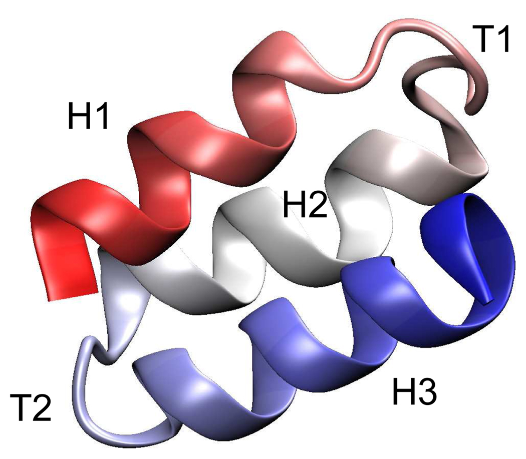
BdpA is a three-helix-bundle protein with a highly symmetrical topology. The three helices (H1, H2 and H3) of comparable length are joined by two turns (T1 and T2) in an antiparallel alignment to form two helix-turn-helix motifs (See Figure 1).

Figure 1.

The native structure of BdpA⁴⁰ shown in cartoon representation. Helix 1, 2 and 3 are colored in red, white and blue respectively. This figure was generated with Visual Molecular Dynamics (VMD).⁴⁹

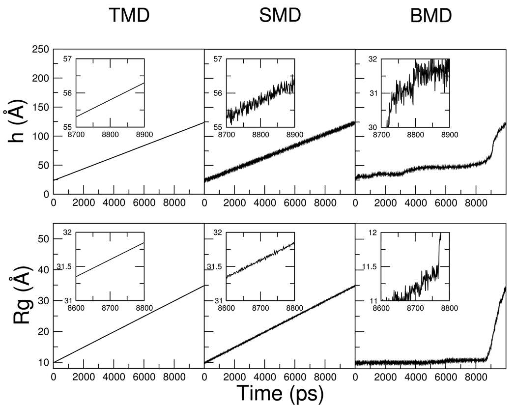
As listed in Table I, a total of 42 unfolding trajectories of BdpA were generated with three perturbation MD methods (BMD/SMD/TMD), two progress variables (end-to-end distance h/radius of gyration R_g), and three different simulation lengths (0.5ns/2ns/10ns). Figure 2 shows the time profiles of the progress variables for representative trajectories generated by the three methods. With TMD, the progress variables scale linearly with time as expected from the holonomic constraint. SMD also generated nearly linear progression curves due to the linear updating of the reference point, but the actual progress variables fluctuate about the linear line. With BMD, the dynamics of the progress variables appear more similar to natural fluctuation in the sense that their values change non-linearly over time. For example in the R_g-perturbed BMD simulation (right bottom panel), the progress variable R_g increases slowly for the first 8 ns until it reaches ~11.5 Å after which it rises with a much steeper slope. This non-linear progression can be utilized to identify possible free energy barriers, because a barrier impedes spontaneous fluctuations along the progress variable and thus longer sampling time is needed to cross it. ^20,21

Figure 2.

The progress variable as a function of time in representative BdpA unfolding trajectories generated by TMD, SMD and BMD. The perturbed progress variable is the end-to-end distance (h) in the top panels and the radius of gyration (R_g) in the bottom panels. Insets show close-ups of a small portion of the progression curves.

The effect of perturbation methods and progress variable on determining path

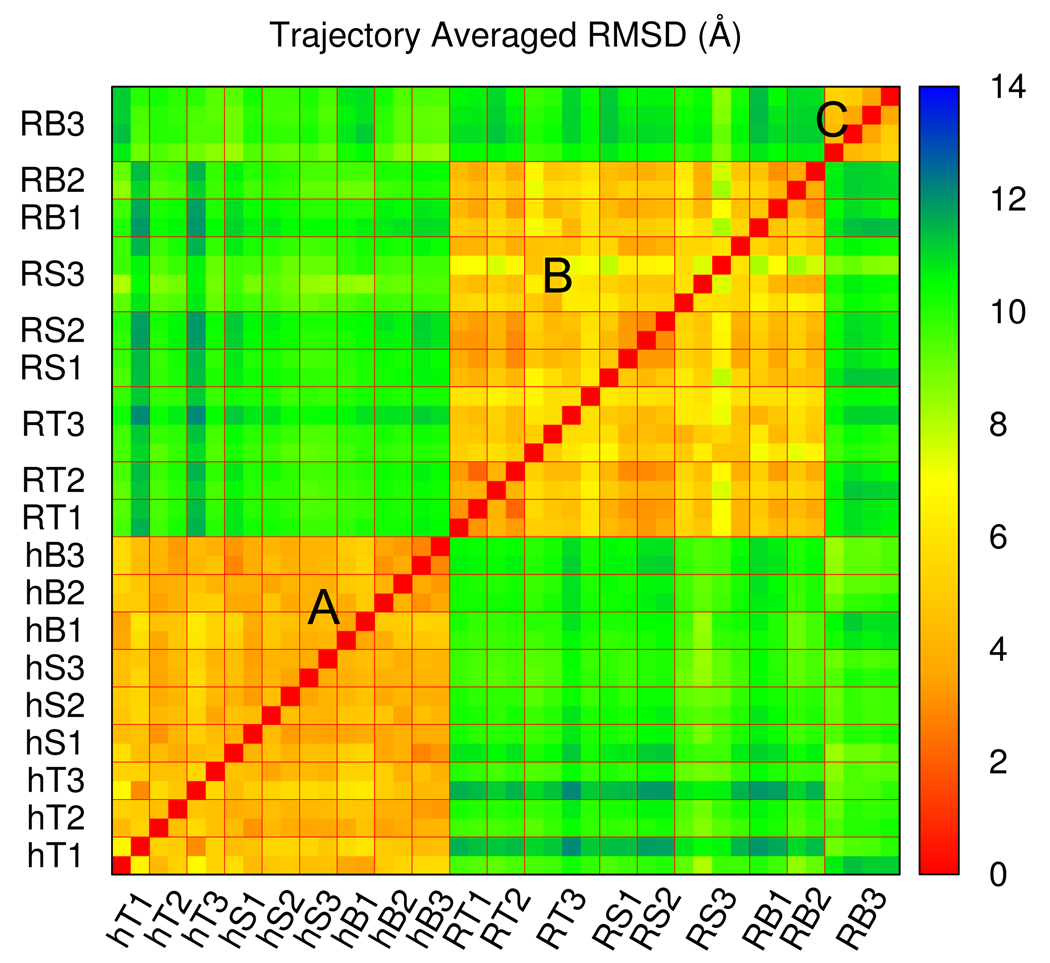
R_g and h were used to guide the unfolding transition of BdpA. Unfolding trajectories, from TMD, SMD and BMD, were compared by the trajectory averaged RMSD values $({\overline{\text{RMSD}}}_{\mathit{\text{ij}}})$, for which the snapshots from each trajectory were binned according to their R_g values. The calculated unfolding trajectories were thus examined as paths connecting conformations in space rather than time evolution of the system. To compare two trajectories, the RMSD was calculated between average structures from each R_g bin, and the RMSD values were averaged over all bins (see Methods for detail). The resulting ${\overline{\text{RMSD}}}_{\mathit{\text{ij}}}$ value measures the overall spatial similarity between two trajectories and the all-against-all evaluation is plotted in the matrix in Figure 3 according to the code shown in Table I. This pairwise similarity matrix shows that, the 42 trajectories naturally fall into three clusters. Interestingly, all h-perturbed trajectories fall into Cluster A, all R_g-perturbed trajectories except RB3 fall into Cluster B, and all R_g-perturbed, RB3 trajectories fall into Cluster C. The groups of trajectories are clearly distinct from each other: The ${\overline{\text{RMSD}}}_{\mathit{\text{ij}}}$ value within any cluster is around 4 Å while that between two different clusters averages near 11 Å.

Figure 3.

The pairwise trajectory averaged RMSD matrix for all BdpA unfolding trajectories. Each color square (pixel) shows the ${\overline{\text{RMSD}}}_{\mathit{\text{ij}}}$ value between a pair of unfolding trajectories. Trajectories are arranged in the same order on both axes so that the matrix is symmetric. Multiple trajectories with the same simulation condition are grouped together by thin lines in red and the coding of simulation conditions is as in Table I. Three clusters can be identified as: Cluster A, all h-perturbed trajectories; Cluster B, all R_g-perturbed trajectories except BMD, 10 ns ones; Cluster C, R_g-perturbed, BMD, 10 ns trajectories

It is apparent from the distinct clustering in Figure 3 that, for the case of BdpA unfolding, the global geometry of the transition path is largely determined by the progress variable being h or R_g, and not by the perturbation method. Comparison of trajectories within a cluster provides no evidence that trajectories generated by either TMD, SMD or BMD differ. The ${\overline{\text{RMSD}}}_{\mathit{\text{ij}}}$ values calculated between unfolding trajectories generated with different perturbation methods are equivalent to values obtained by comparing multiple runs by the same method and simulation length.

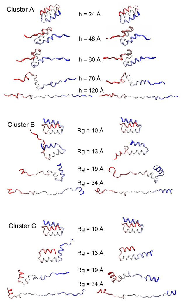
Inspecting all trajectories with the visualization program VMD⁴⁹ identified the global features shared by all members from the same cluster. These common features are shown in Figure 4 by two representative trajectories for unfolding from each cluster. In Cluster A trajectories, the protein unfolds by first extending and unwinding H1 and H3 from the ends. Breaking of the H1–H2 and H2–H3 interhelical contacts follows as a result of the stretching at the ends by perturbing h. The protein then extends into a linear chain. In Cluster B trajectories, the H1–H2 hairpin always opens up with a flipping of H1 at an early stage of unfolding. The opening up of H2–H3 hairpin occurs later. In contrast, these two events happen in the opposite order in Cluster C, where H3 flips to lose contact with H2 earlier than the separation of H1 and H2.

Figure 4.

Snapshots unfolded to different extents are shown for representative trajectories from each cluster. Helix 1, 2 and 3 are shown in red, white and blue, respectively. These ribbon graphs show the sequence of key events involved in the unfolding, including the unwinding of individual helices and the interruption of different tertiary contacts. Two trajectories are shown for each cluster to exemplify variations within a cluster.

The stronger dependence of the transition path on the progress variable than the method is evident from a similarity shared by Cluster B and C paths regardless of the big RMSD between them. In these two clusters, the opening up of one of the two hairpins (H1–H2 in B and H2–H3 in C) happens as the first step of unfolding. This common feature is consistent with the external forces imposed by R_g perturbation in that the opening up of a hairpin will result in a big increase in R_g. In contrast, in all Cluster A trajectories the unwinding of H1 and H3 from the ends precedes the breaking of the hairpin structure. This alternative pathway is also consistent with the pulling forces at the ends imposed by the end-to-end distance, h, perturbation.

Trajectories from the same cluster follow a common global trend but still display variability in structural details. One example of this variability is that H2 breaks in the middle (Figure 4 top, right, h=60 Å) and reforms (h=76 Å) before it is unwound in some but not all Cluster A trajectories. Another example is that the unwinding of H1 accompanies H1–H2 separation in some but not all Cluster B trajectories (Figure 4 middle, left). Similar differences are also observed in Cluster C trajectories (Figure 4 bottom). These local differences are not specific to a certain perturbation method. However, in general, the variability of R_g trajectories is greater than that of h trajectories in two aspects. First, R_g perturbation resulted in two distinct clusters (B and C) whereas h perturbation resulted in a single one (A). Second, R_g-perturbed trajectories have higher intra-cluster ${\overline{\text{RMSD}}}_{\mathit{\text{ij}}}$ values, as shown by more yellow-green elements in the similarity matrix in Cluster B than in A. This greater variability produced by the R_g bias is consistent with the more divergent nature of its corresponding forces.

BMD 10 ns R_g-perturbed trajectories form a distinct cluster

Within R_g-perturbed trajectories, the RB3 trajectories generated by BMD in 10 ns (the longest time, with the smallest force constant) form a distinct group Cluster C. As mentioned earlier, they differ from other R_g-perturbed trajectories in first opening up hairpin H2–H3 instead of H1–H2. In the three-helix-bundle structure of BdpA, both H1 and H3 form antiparallel interhelical tertiary interactions with H2, resulting in a nearly symmetrical topology. The interruption of one of these two tertiary interactions during unfolding can be considered as a breaking of symmetry. ³⁸ Assuming this symmetry to be perfect, its disruption should occur randomly at H1–H2 or H2–H3 as a result of the chaotic nature of molecular dynamics. However, here we observe H2–H3 breaking only in RB3 trajectories. This observation suggests an underlying picture in which both the protein’s internal interactions and the external perturbation forces are slightly asymmetric and favor different symmetry breaking positions, and the balance between the two asymmetric factors determines which contact breaks first. With short simulation lengths, the perturbation strength was high and all perturbation methods generated H1–H2 breaking trajectories only. As the simulation time increased, the perturbation strengths for all three methods were decreased, which would potentially cause a change of the balance between the external perturbation and internal interaction. Interestingly, in the longest simulation time (10 ns), only BMD sampled the alternative pathway, suggesting that BMD gives a smaller effective perturbation in the same simulation time. This smaller effective perturbation can be explained by the nonlinear sampling of BMD. With BMD, a larger portion of the total sampling time is spent before barrier-crossing events. Because barrier crossing events are the critical events in determining which path to follow, BMD renders a weaker perturbation during these important events and thus sampled the alternative pathway in the longest simulation time.

Cluster C has lower PMF values than Cluster B

The TMD, SMD and BMD perturbation methods were further examined for their ability to generate physically relevant transition paths by an assessment of the energetics of the unfolding trajectories. Because instantaneous energies are sensitive to local structural changes and contain high level of noise, they were not used to compare the energetics of the trajectories. Instead, a potential of mean force (PMF) curve was calculated for a trajectory by using umbrella sampling and WHAM with snapshots taken from the trajectory as initial coordinates. The PMF curves aim to characterize the path obtained from trajectories generated for set conditions of perturbation method and length of simulation. It is recognized that there is variation among the curves because of limited sampling in the energy averaging on a rugged conformational landscape. Nonetheless, the PMF curves were found to be useful for comparative purposes.

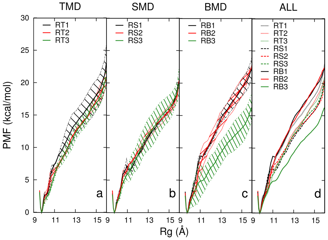
The PMF with respect to R_g were calculated for all R_g-perturbed trajectories (Cluster B and C) over the R_g range of 9.5 Å to 16.0 Å (see Methods for details). Figure 5 shows the average PMF and its variance as a function of R_g for each simulation condition. The average and variance were calculated from multiple (two to four) independent trajectories for each simulation condition and shown in Figure 5(a–c). Only the averaged PMF is shown in Figure 5(d) for clarity. All PMF curves share the same overall shape. There is a minimum at R_g=9.8 Å, which is the R_g of the native structure. There are no other minima along the curves, a behavior also observed in BMD unfolding of the Fn3 domain.⁶

Figure 5.

The potential of mean force (PMF) as a function of R_g for R_g-perturbed BdpA unfolding paths. The first three panels show the PMF curves, labeled by the codes shown in Table I, for each time length for (a) TMD, (b) SMD and (c) BMD. An average curve is calculated from PMF profiles of multiple trajectories (two to four) with the same simulation condition, and the shaded area shows the variance. (d) Average PMF curves.

Paths generated by RB3 trajectories (Cluster C) have the lowest PMF for R_g values > 11 Å, indicating an energetically more favorable unfolding path. Nevertheless, a comparison of shorter (0.5 ns and 2 ns) trajectories reveals that those generated by BMD are not more energetically favorable than SMD or TMD generated trajectories. Interestingly, the structural difference between RB3 and other R_g-perturbed trajectories for Rg > 11 Å is the breaking of H2–H3 contact or that of H1–H2. It is likely that the difference in PMF between RB3 and other trajectories is a reflection of the two different unfolding pathways described earlier. The fact that RB3 paths have lower PMF curves is also consistent with the earlier discussed notion that BMD renders a smaller effective perturbation in the same simulation time, thus samples an alternative, lower free energy pathway.

3.2 Lyn Activation/Deactivation

The second example system on which the three perturbation methods were tested is the conformational transition of the Lyn kinase CD. This process is a transition between two end states with well defined structures, in contrast to the unfolding of BdpA.

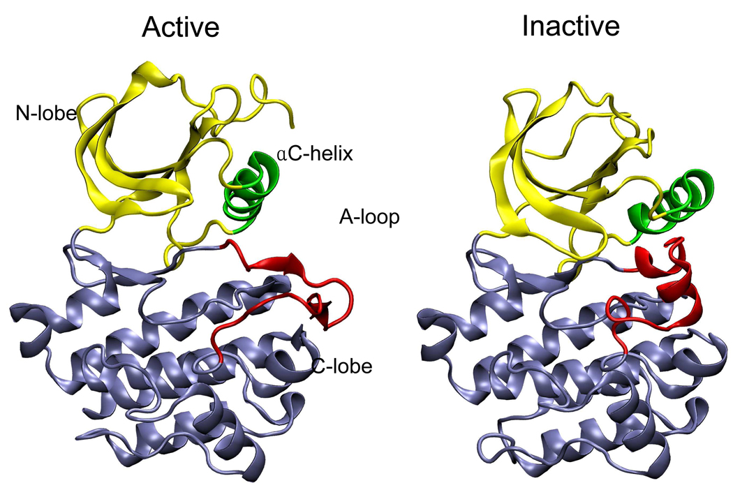
The catalytic domain of Src-family kinases, such as Lyn CD, adopts different conformations in the active and inactive states shown in Figure 6. Major conformational changes of the CD upon activation are the opening of the cleft between the N- and C-terminal lobes (N-lobe and C-lobe), the rotation and translation of the αC helix, and rearrangement of the activation loop (A-loop). The 20-residue long A-loop undergoes the most complex rearrangement. It adopts an extended conformation in the active state, whereas in the inactive state, it folds back into the catalytic cleft, forming two short α helices.

Figure 6.

A comparison of the catalytic domain conformations of a Src kinase Lyn in the active (left) and inactive (right) states. The structures are from equilibrium molecular dynamics simulations²³ initiated with coordinates obtained by homology modeling with Lck⁴³ and Hck⁴⁴ crystal structures. Upon activation, the N-lobe (yellow) and C-lobe (blue) move apart, the helix C (green) moves and rotates inward, and the A-loop (red) deforms from two short helices to extended structure.

Both activation and deactivation transition paths were calculated for the Lyn CD using the three perturbation MD methods. The two target structures were obtained by equilibrium MD with explicit water molecules initiated from homology modeled coordinates (see Methods). All three perturbation methods were applied with the MSID progress variable (see Methods for definition) to guide the transition to the target structure. Trajectories perturbing the root mean square deviation (RMSD) were also calculated with TMD. Details about the simulations are listed in Table II.

Path completeness

Unlike unfolding, the conformational transition process modeled in this example has a defined target configuration. By definition, TMD guarantees that the target configuration will be reached, while SMD only restrains the system to the target value with a defined force constant. With BMD, even the final reference point ρ₀ is not guaranteed to be the target value in a certain amount of time because it depends on spontaneous fluctuations of the system.

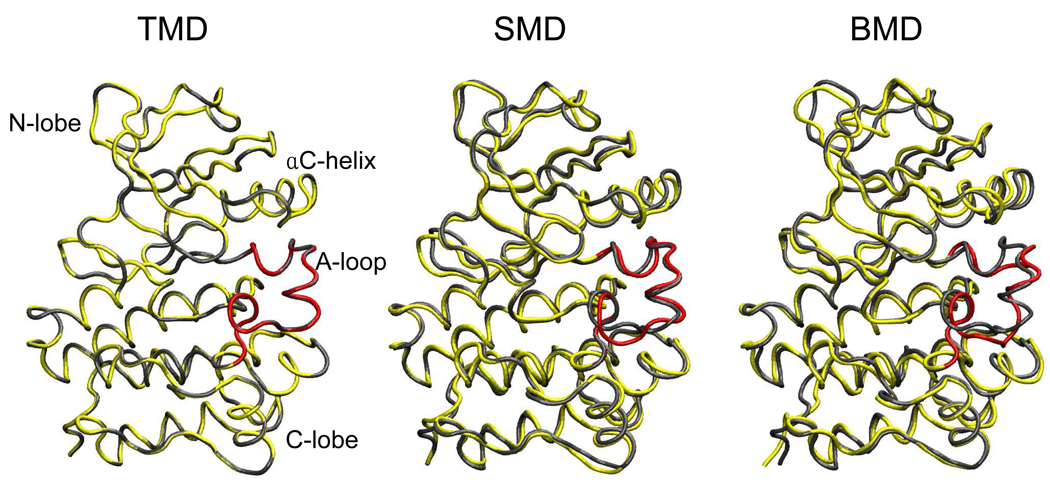
The final states of Lyn generated by the three methods are in accord with the above expectations. Figure 7 shows a superposition based on all heavy atoms of the target structure and the structure at the end of the perturbation MD run for representative deactivation simulations. TMD guided the transition to the exact target. With SMD, the final structure and the target configuration differ slightly (overall RMSD = 1.2 Å and A-loop RMSD = 2.8 Å), with differences in several backbone torsion angles in the C-terminal region of the A-loop. The final structure generated by BMD has the largest deviation (overall RMSD = 1.9 Å, A-loop RMSD = 3.4 Å) from the target of the three perturbation methods. The major deviation is again in the A-loop region but also involves differences at the secondary structure level. Specifically, the two short A-loop helices do not form.

Figure 7.

Final structures of Lyn CD deactivation trajectories generated by TMD, SMD and BMD. These calculated final structures are shown in yellow except for the A-loop colored in red, whereas the native inactive structure, i.e. the target configuration is shown in gray.

The effect of perturbation methods and progress variable on determining path

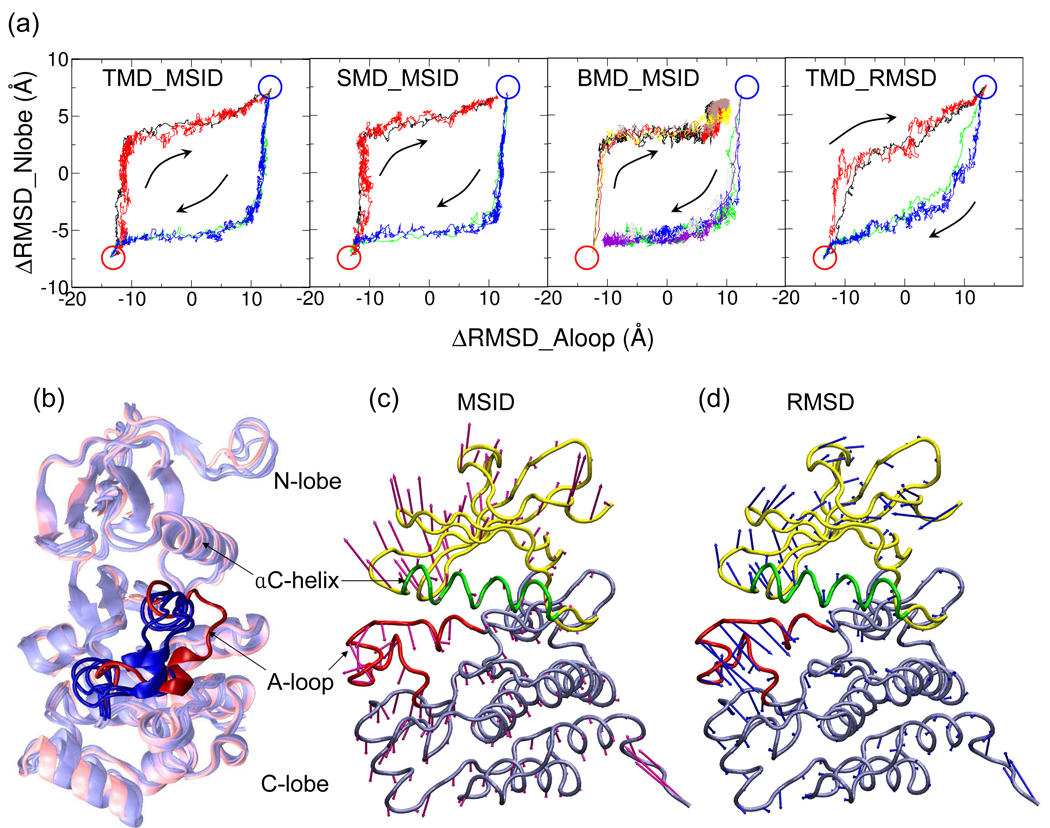
Figure 8(a) shows the projection of all 20 trajectories onto two coordinates: ΔRMSD of the A-loop and ΔRMSD of the N-lobe. ΔRMSD_Aloop and ΔRMSD_Nlobe of a configuration is defined as the difference between the RMSD of this configuration to the active structure and the RMSD to the inactive structure for the heavy atoms of the A-loop (residues 406 to 526, c-Src numbering) and the N-lobe (residues 261 to 301 and 317 to 341), respectively, with the C-lobe superimposed.

Figure 8.

(a) Lyn CD activation/deactivation trajectories projected on the plane of ΔRMSD of the N-lobe and ΔRMSD of the A-loop. For each panel, multiple trajectories are shown in different colors. See Table II for color coding. ΔRMSD = RMSD(to active)−RMSD(to inactive), super-imposing the C-lobe of the protein. The active and inactive configurations are labeled by red and blue circles respectively, and the transition directions are indicated by arrows. (b) Four snapshots with the N-lobe opened to the same extent from four Lyn CD activation trajectories generated by TMD-MSID, SMD-MSID, BMD-MSID and TMD-RMSD. For each trajectory, the first snapshot that reaches ΔRMSD_Nlobe = −5 Å is shown. The three snapshots with MSID as the progress variable are colored in blue whereas the one with MSID as the progress variable is colored in red. The A-loop region is shown in solid cartoon representation while the rest of the protein is shown as transparent. (c–d) External forces acting on Lyn CD at the beginning of activation by perturbing MSID (c) or RMSD (d). The forces are averaged for each residue and scaled so that their average magnitude are the same in both cases. RMSD induces relatively greater forces on the A-loop region compared to that MSID does.

Trajectories generated with the same progress variable, MSID, using three perturbation methods are similar on the two-dimensional ΔRMSD surface, as shown in the first three panels of Figure 8(a). These trajectories follow two different major paths depending on their direction being activation or deactivation. The two motions take place in two distinct steps that follow each other, as indicated by a sudden change in slope once one change is completed. For either direction, the lobe-lobe motion occurs before the rearrangement of the A-loop and the forward path is not the opposite of the reverse path. This behavior indicates that the energy barrier for the hinge-like lobe-lobe motion is lower than that for A-loop rearrangement which involves a change in secondary structure, and suggests that the global geometry of a transition path is dependent not only on the perturbation force, but also on the ease of the motions induced by the perturbation force. The observation of globally similar paths for all MSID-perturbed trajectories suggests that the dependence of the path on the perturbation method is minor, even though BMD generated deactivation paths that slightly differ from those generated by TMD and SMD at the end (Figure 8(a), panel 3) due to a delayed motion of the αC helix.

The fourth combination of perturbation method and progress variable, TMD with the RMSD progress variable, generated paths globally different from all MSID paths. On the two-dimensional surface, these paths progress more linearly rather than stepwise, which suggests that the N-lobe and the A-loop move toward the target structure with a higher degree of cooperativity. This result is again in accord with the notion that the global path is largely determined by the choice of the progress variable.

The difference in the linearity between paths generated with MSID and RMSD as the progress variable can be seen structurally in snapshots from representative activation trajectories. Figure 8(b) shows an overlay of four snapshots from activation trajectories generated by the four combinations of perturbation method and progress variable. Upon activation, both the N-lobe and the A-loop open up from a closed conformation, and the four snapshots were chosen so that their N-lobes are opened to the same extent: ΔRMSD_Nlobe = −5Å. Figure 8(b) shows that in the snapshot generated by perturbing RMSD (red), the A-loop motion has progressed further toward the active conformation while A-loops of the other snapshots generated by perturbing MSID (blue) remain close to the inactive state. It is worth noting that both MSID and RMSD are global measurements of the distance between two structures, and therefore as progress variables they are less distinct than h and R_g. Nonetheless, the subtle distinction does result in visible differences between generated paths again showing the sensitivity of the perturbation MD methods to the choice of progress variable.

To examine the reason for the generation of different paths with the two progress variables, the forces imposed by perturbation on MSID or RMSD on each residue at the beginning of the activation are shown in Figure 8(c,d). The magnitudes of the forces are scaled so that their average magnitude for the molecule is the same. It can be seen in the visualization that RMSD induces relatively greater initial forces on the A-loop region compared to the forces imposed by MSID. The variation and difference in direction in the force vectors explains the observed differences between the paths. Simulations perturbing the RMSD progress variable were not carried out with BMD and SMD, but results similar to that observed by TMD are expected.

4 Conclusions and Discussion

In the present study, we compared TMD, SMD and BMD methods for guiding conformational transitions with external perturbation. Two distinct transition systems were explored: the unfolding of BdpA with implicit solvation and a heterogeneous end state, and the activation of Lyn CD in explicit water with two well-defined end states. Results from the three perturbation methods with two choices of progress variable and varying simulation length or biasing force constant showed that the perturbation methods generate similar transition paths for a given progress variable, as defined by global structural features. On the other hand, the path was strongly dependent on the choice of progress variable. Specifically, choosing to perturb R_g or h for unfolding BdpA determines whether the protein unfolds by stretching from the ends or by opening up one of the two inter-helical contacts. Also, choosing to perturb MSID or RMSD to guide the conformational change of Lyn CD affects the cooperativity of the movements of its N-lobe and A-loop.

The path dependence on the progress variable was observed to be related to the direction and relative magnitude of the perturbation force, and these were the dominant influence regardless of the perturbation method. The alternative forces induce different motions of the molecule in certain directions, and together with the intrinsic ease of these motions, determine the transition path. In most cases, it is not clear that a priori knowledge can be used to decide which progress variable is a good reaction coordinate.

Although the three methods generated similar paths in terms of the global structural features for a given progress variable in most cases, the RB3 BdpA unfolding simulations generated by BMD with the lowest force constant, identified an alternative class of paths, whereas longer SMD and TMD simulations generated similar paths to those generated by shorter simulations. The fact that this alternative class of paths is more energetically favorable is likely due to the softer and nonlinear perturbation rendered by BMD. BMD realizes a nonlinear updating scheme for moving along the progress variable, and thus the perturbation strength varies along a trajectory. In simulations of the same total length, BMD spends a greater amount of time going up a barrier than going down a slope. Thus the perturbation strength is comparatively low with BMD when the system searches for an easy route to overcome a free energy barrier. It should be noted that this nonlinear updating scheme of BMD would not guarantee the sampling of globally lower free energy paths, because an effectively lower perturbation strength only helps find an easy route to cross a local free energy barrier, which may or may not be a part of the global optimal path. In fact, the blindness to global features of the free energy surface is a common problem shared by all three perturbation methods.

In the conformational transition of Lyn CD, the backward paths are not the reverse copies of the forward paths with all three perturbation methods. This apparent violation of the microscopic reversibility suggests that the nonequilibrium results obtained with the perturbation MD methods do not approach the equilibrium results at the time lengths examined in our simulations. With the perturbation methods in the nonequilibrium scenario, the sequence of events along a path is determined by a combined effect of the perturbation and the internal ease of certain motions. Under the perturbation, the parts that feel the strongest perturbation and the weakest hindrance move toward the target first. Due to this lack of reversibility, caution should be taken when interpreting perturbation MD results to infer features such as sequence of events. Nevertheless, some insight on the ease of a certain motion can be obtained with these perturbation methods.

Global and/or local structural properties of the proteins should be considered when choosing a perturbation MD method. As our simulations on the conformational transition of Lyn CD show, BMD trajectories can be trapped in local minima in the presence of significant energy barriers (such as the A-loop rearrangement), preventing the system from arriving at the target conformation. TMD and, for the most part, SMD ensure the completeness of the transition, although the likelihood of the path followed by TMD has not been assessed here. SMD closely resembles the AFM experiment, and is preferred when direct analogy is desired. Further use of SMD allows the application of the Jarzynski’s equality to calculate equilibrium free energy differences. ⁵⁰ The Jarzynski’s equality requires the external perturbation to be a component of the Hamiltonian as an explicit function of time, a condition satisfied by the perturbation form of SMD but by neither TMD nor BMD.⁵¹

Abbreviations and Symbols

BMD

Biased Molecular Dynamics

TMD

targeted molecular dynamics

SMD

Steered Molecular Dynamics

ρ

progress variable

h

end-to-end distance

R_g

radius of gyration

RMSD

Root Mean Square Deviation

MSID

Mean Square Internal Deviation.

References

- 1.Schlitter J, Engels M, Kruger P, Jacoby E, Wollmer A. Mol. Simul. 1993;10:291–308. [Google Scholar]
- 2.Schlitter J, Engels M, Kruger P. J. Mol. Graph. 1994;12:84–89. doi: 10.1016/0263-7855(94)80072-3. [DOI] [PubMed] [Google Scholar]
- 3.Grubmueller H, Heymann B, Tavan P. Science. 1996;271:997–999. doi: 10.1126/science.271.5251.997. [DOI] [PubMed] [Google Scholar]
- 4.Leech J, Prins J, Hermans J. IEEE Comp. Sci. Eng. 1996;3:38–45. [Google Scholar]
- 5.Marchi M, Ballone P. J. Chem. Phys. 1999;110:3697–3702. [Google Scholar]
- 6.Paci E, Karplus M. J. Mol. Biol. 1999;288:441–459. doi: 10.1006/jmbi.1999.2670. [DOI] [PubMed] [Google Scholar]
- 7.Izrailev S, Stepaniants S, Balsera M, Oono Y, Schulten K. Biophys. J. 1997;72:1568–1581. doi: 10.1016/S0006-3495(97)78804-0. [DOI] [PMC free article] [PubMed] [Google Scholar]
- 8.Lu H, Isralewitz B, Krammer A, Vogel V, Schulten K. Biophys. J. 1998;75:662–671. doi: 10.1016/S0006-3495(98)77556-3. [DOI] [PMC free article] [PubMed] [Google Scholar]
- 9.Krammer A, Lu H, Isralewitz B, Schulten K, Vogel V. Proc. Natl. Acad. Sci. U. S. A. 1999;96:1351–1356. doi: 10.1073/pnas.96.4.1351. [DOI] [PMC free article] [PubMed] [Google Scholar]
- 10.Marszalek PE, Lu H, Li HB, Carrion-Vazquez M, Oberhauser AF, Schulten K, Fernandez JM. Nature. 1999;402:100–103. doi: 10.1038/47083. [DOI] [PubMed] [Google Scholar]
- 11.Law RJ, Munson K, Sachs G, Lightstone FC. Biophys. J. 2008;95:2739–2749. doi: 10.1529/biophysj.107.128025. [DOI] [PMC free article] [PubMed] [Google Scholar]
- 12.Swift RV, McCammon JA. Biochemistry. 2008;47:4102–4111. doi: 10.1021/bi8000209. [DOI] [PubMed] [Google Scholar]
- 13.Zou J, Wang Y-D, Ma F-X, Xiang M-L, Shi B, Wei Y-Q, Yang S-Y. Proteins: Struct. Funct. Bioinf. 2008;72:323–332. doi: 10.1002/prot.21928. [DOI] [PubMed] [Google Scholar]
- 14.Apostolakis J, Ferrara P, Caflisch A. J. Chem. Phys. 1999;110:2099–2108. [Google Scholar]
- 15.Bui JM, McCammon JA. Proc. Natl. Acad. Sci. U. S. A. 2006;103:15451–15456. doi: 10.1073/pnas.0605355103. [DOI] [PMC free article] [PubMed] [Google Scholar]
- 16.Ferrara P, Apostolakis J, Caflisch A. J. Phys. Chem. B. 2000;104:4511–4518. [Google Scholar]
- 17.Ma J, Karplus M. Proc. Natl. Acad. Sci. U. S. A. 1997;94:11905–11910. doi: 10.1073/pnas.94.22.11905. [DOI] [PMC free article] [PubMed] [Google Scholar]
- 18.Ferrara P, Apostolakis J, Caflisch A. Proteins: Struct. Funct. Genet. 2000;39:252–260. doi: 10.1002/(sici)1097-0134(20000515)39:3<252::aid-prot80>3.0.co;2-3. [DOI] [PubMed] [Google Scholar]
- 19.Paci E, Caflisch A, Pluckthun A, Karplus M. J. Mol. Biol. 2001;314:589–605. doi: 10.1006/jmbi.2001.5103. [DOI] [PubMed] [Google Scholar]
- 20.Morra G, Hodoscek M, Knapp EW. Proteins: Struct. Funct. Genet. 2003;53:597–606. doi: 10.1002/prot.10344. [DOI] [PubMed] [Google Scholar]
- 21.Li Y, Zhou Z, Post CB. Proc. Natl. Acad. Sci. U. S. A. 2005;102:7529–7534. doi: 10.1073/pnas.0408749102. [DOI] [PMC free article] [PubMed] [Google Scholar]
- 22.Stultz CM. Protein Sci. 2006;15:2166–2177. doi: 10.1110/ps.062124606. [DOI] [PMC free article] [PubMed] [Google Scholar]
- 23.Ozkirimli E, Post CB. Protein Sci. 2006;15:1051–1062. doi: 10.1110/ps.051999206. [DOI] [PMC free article] [PubMed] [Google Scholar]
- 24.Levinson NM, Kuchment O, Shen K, Young MA, Koldobskiy M, Karplus M, Cole PA, Kuriyan J. PLoS Biol. 2006;4:e144. doi: 10.1371/journal.pbio.0040144. [DOI] [PMC free article] [PubMed] [Google Scholar]
- 25.Kastenholz MA, Schwartz TU, Hünenberger PH. Biophys. J. 2006;91:2976–2990. doi: 10.1529/biophysj.106.083667. [DOI] [PMC free article] [PubMed] [Google Scholar]
- 26.Perdih A, Kotnik M, Hodoscek M, Solmajer T. Proteins: Struct. Funct. Bioinf. 2007;68:243–254. doi: 10.1002/prot.21374. [DOI] [PubMed] [Google Scholar]
- 27.Ozkirimli E, Yadav SS, Miller WT, Post CB. Protein Sci. 2008;17:1871–1880. doi: 10.1110/ps.037457.108. [DOI] [PMC free article] [PubMed] [Google Scholar]
- 28.Tikhonova IG, Best RB, Engel S, Gershengorn MC, Hummer G, Costanzi S. J. Am. Chem. Soc. 2008;130:10141–10149. doi: 10.1021/ja0765520. [DOI] [PMC free article] [PubMed] [Google Scholar]
- 29.Zhong W, Guo W, Ma S. FEBS Lett. 2008;582:3320–3324. doi: 10.1016/j.febslet.2008.08.020. [DOI] [PubMed] [Google Scholar]
- 30.Matrai J, Jonckheer A, Joris E, Kruger P, Carpenter E, Tuszynski J, Maeyer MD, Engelborghs Y. Eur. Biophys. J. 2008;38:13–23. doi: 10.1007/s00249-008-0348-2. [DOI] [PubMed] [Google Scholar]
- 31.Carrion-Vazquez M, Li H, Lu H, Marszalek PE, Oberhauser AF, Fernandez JM. Nat. Struct. Biol. 2003;10:738–743. doi: 10.1038/nsb965. [DOI] [PubMed] [Google Scholar]
- 32.Sato S, Religa TL, Fersht AR. J. Mol. Biol. 2006;360:850–864. doi: 10.1016/j.jmb.2006.05.051. [DOI] [PubMed] [Google Scholar]
- 33.Vu DM, Myers JK, Oas TG, Dyer RB. Biochemistry. 2004;43:3582–3589. doi: 10.1021/bi036203s. [DOI] [PubMed] [Google Scholar]
- 34.Myers JK, Oas TG. Nat. Struct. Biol. 2001;8:552–558. doi: 10.1038/88626. [DOI] [PubMed] [Google Scholar]
- 35.Guo Z, Brooks CL, Boczko EM. Proc. Natl. Acad. Sci. U. S. A. 1997;94:10161–10166. doi: 10.1073/pnas.94.19.10161. [DOI] [PMC free article] [PubMed] [Google Scholar]
- 36.Garcia AE, Onuchic JN. Proc. Natl. Acad. Sci. U. S. A. 2003;100:13898–13903. doi: 10.1073/pnas.2335541100. [DOI] [PMC free article] [PubMed] [Google Scholar]
- 37.Cheng S, Yang Y, Wang W, Liu H. J. Phys. Chem. B. 2005;109:23645–23654. doi: 10.1021/jp0517798. [DOI] [PubMed] [Google Scholar]
- 38.Itoh K, Sasai M. Proc. Natl. Acad. Sci. U. S. A. 2006;103:7298–7303. doi: 10.1073/pnas.0510324103. [DOI] [PMC free article] [PubMed] [Google Scholar]
- 39.Binnig G, Quate CF, Gerber C. Phys. Rev. Lett. 1986;56:930–933. doi: 10.1103/PhysRevLett.56.930. [DOI] [PubMed] [Google Scholar]
- 40.Gouda H, Torigoe H, Saito A, Sato M, Arata Y, Shimada I. Biochemistry. 1992;31:9665–9672. doi: 10.1021/bi00155a020. [DOI] [PubMed] [Google Scholar]
- 41.Im W, Lee MS, Brooks CL. J. Comput. Chem. 2003;24:1691–1702. doi: 10.1002/jcc.10321. [DOI] [PubMed] [Google Scholar]
- 42.Brooks BR, Bruccoleri RE, Olafson BD, States DJ, Swaminathan S, Karplus M. J. Comput. Chem. 1983;4:187–217. [Google Scholar]
- 43.Yamaguchi H, Hendrickson WA. Nature. 1996;384:484–489. doi: 10.1038/384484a0. [DOI] [PubMed] [Google Scholar]
- 44.Schindler T, Sicheri F, Pico A, Gazit A, Levitzki A, Kuriyan J. Mol. Cell. 1999;3:639–648. doi: 10.1016/s1097-2765(00)80357-3. [DOI] [PubMed] [Google Scholar]
- 45.Paci E, Smith LJ, Dobson CM, Karplus M. J. Mol. Biol. 2001;306:329–347. doi: 10.1006/jmbi.2000.4337. [DOI] [PubMed] [Google Scholar]
- 46.Markwick PRL, Doltsinis NL, Schlitter J. J. Chem. Phys. 2007;126:045104. doi: 10.1063/1.2431177. [DOI] [PubMed] [Google Scholar]
- 47.Torrie GM, Valleau JP. J. Comp. Phys. 1977;23:187–199. [Google Scholar]
- 48.Ferrenberg AM, Swendsen RH. Phys. Rev. Lett. 1989;63:1195–1198. doi: 10.1103/PhysRevLett.63.1195. [DOI] [PubMed] [Google Scholar]
- 49.Humphrey W, Dalke A, Schulten K. J. Mol. Graph. 1996;14:33–38. 27–28. doi: 10.1016/0263-7855(96)00018-5. [DOI] [PubMed] [Google Scholar]
- 50.West DK, Olmsted PD, Paci E. J. Chem. Phys. 2006;125:204909. doi: 10.1063/1.2393232. [DOI] [PubMed] [Google Scholar]
- 51.Jarzynski C. Phys. Rev. Lett. 1997;78:2690. [Google Scholar]