Correlations in spiking neuronal networks with distance dependent connections

Abstract

Can the topology of a recurrent spiking network be inferred from observed activity dynamics? Which statistical parameters of network connectivity can be extracted from firing rates, correlations and related measurable quantities? To approach these questions, we analyze distance dependent correlations of the activity in small-world networks of neurons with current-based synapses derived from a simple ring topology. We find that in particular the distribution of correlation coefficients of subthreshold activity can tell apart random networks from networks with distance dependent connectivity. Such distributions can be estimated by sampling from random pairs. We also demonstrate the crucial role of the weight distribution, most notably the compliance with Dales principle, for the activity dynamics in recurrent networks of different types.

Introduction

The collective dynamics of balanced random networks was extensively studied, assuming different neuron models as constituting dynamical units (van Vreeswijk and Sompolinsky 1996, 1998; Brunel and Hakim 1999; Brunel 2000; Mattia and Del Guidice 2002; Timme et al. 2002; Mattia and Del Guidice 2004; Kumar et al. 2008b; Jahnke et al. 2008; Kriener et al. 2008).

Some of these models have in common that they assume random network topologies with a sparse connectivity ϵ ≈ 0.1 for a local, but large neuronal network, embedded into an “external” population that supplies unspecific white noise drive to the local network. These systems are considered as minimal models for cortical networks of about 1 mm³ volume, because they can display activity states similar to those observed invivo, such as asynchronous irregular spiking. Yet, as recently reported (Song et al. 2005; Yoshimura et al. 2005; Yoshimura and Callaway 2005), local cortical networks are characterized by a circuitry, which is specific and hence, non-random even on a small spatial scale. Since it is still impossible to experimentally uncover the whole coupling structure of a neuronal network, it is necessary to infer some of its features from its activity dynamics. Timme (2007) e.g. studied networks of N coupled phase oscillators in a stationary phase locked state. In these networks it is possible to reconstruct details of the network coupling matrix (i.e. topology and weights) by slightly perturbing the stationary state with different driving conditions and analyzing the network response. Here, we focus on both network structure and activity dynamics in spiking neuronal networks on a statistical level. We consider several abstract model networks that range from strict distance dependent connectivity to random topologies, and examine their activity dynamics by means of numerical simulation and quantitative analysis. We focus on integrate-and-fire neurons arranged on regular rings, random networks, and so-called small-world networks (Watts and Strogatz 1998). Small-world structures seem to be optimal brain architectures for fast and efficient inter-areal information transmission with potentially low metabolic consumption and wiring costs due to a low characteristic path length ℓ (Chklovskii et al. 2002), while at the same time they may provide redundancy and error tolerance by highly recurrent computation (high clustering coefficient , for the general definitions of ℓ and , cf. e.g. Watts and Strogatz (1998), Albert and Barabasi (2002)). Also on an intra-areal level cortical networks may have pronounced small-world features as was shown in simulations by Sporns and Zwi (2004), who assumed a local Gaussian connection probability and a uniform long-range connection probability for local cortical networks, assumptions that are in line with experimental observations (Hellwig 2000; Stepanyants et al. 2007). Network topology is just one aspect of neuronal network coupling, though. Here, we also demonstrate the crucial role of the weight distribution, especially with regard to the notion that all inhibitory neurons project only hyperpolarizing synapses onto their postsynaptic targets, and excitatory neurons only project depolarizing synapses. This assumption is sometimes referred to as Dale′s principle (Li and Dayan 1999; Dayan and Abbott 2001; Hoppensteadt and Izhikevich 1997). Strikingly, this has strong implications for the dynamical states of random networks already (Kriener et al. 2008). Yet, the main focus of the present study is put on the distance dependence and overall distribution of correlation coefficients. Especially the joint statistics of subthreshold activity, i.e. correlations and coherences between the incoming currents that neurons integrate, has been shown to contain elusive information about network parameters, e.g. the mean connectivity in random networks (Tetzlaff et al. 2007).

The paper is structured as follows: In Section 2 we give a short description of the details of the neuron model and the simulation parameters used throughout the paper. In Section 3 we introduce the notion of small-world networks and in Section 4 we discuss features of the activity dynamics in dependence of the topology. In ring and small-world networks groups of neighboring neurons tend to spike highly synchronously, while the population dynamics in random networks is asynchronous-irregular. To understand the source of this differences in the population dynamics, we analyze the correlations of the inputs of neurons in dependence of the network topology. Section 5 is devoted to the theoretical framework we apply to calculate the input correlations in dependence of the pairwise distance in sparse ring (Section 5.1) and small-world networks (Section 5.2). In Section 6 we finally derive the full distribution of correlation coefficients for ring and random networks. Random networks have rather narrow distributions centered around the mean correlation coefficient, while sparse ring and small-world networks have distributions with heavy tails. This is due to the high probability to share a common input partner if the neurons are topological neighbors, and very low probability if they are far apart, yielding distributions with a few high correlation coefficients and many small ones. This offers a way to potentially distinguish random topologies from topologies with small-world features by their subthreshold activity dynamics on a statistical level.

Neuronal dynamics and synaptic input

The neurons in the network of size N are modeled as leaky integrate-and-fire point neurons with current-based synapses. The membrane potential dynamics V_k(t), k ∈ {1,...,N} of the neurons is given by

1

with membrane resistance R and membrane time constant . Whenever V_k(t) reaches the threshold θ, a spike is emitted, V_k(t) is reset to , and the neuron stays refractory for a period . Synaptic inputs

2

from the local network are modeled as δ-currents. Whenever a presynaptic neuron i fires an action potential at time t_il, it evokes an exponential postsynaptic potential (PSP) of amplitude

3

after a transmission delay Δ that is the same for all synapses. Note that multiple connections between two neurons and self-connections are excluded in this framework. In addition to the local input, each neuron receives an external Poisson current mimicking inputs from other cortical areas or subcortical regions. The total input is thus given by

4

Parameters

The neuron parameters are set to ms, R = 80 MΩ, J = 0.1 mV, and Δ = 2 ms. The firing threshold θ is 20 mV and the reset potential mV. After a spike event, the neurons stay refractory for ms. If not stated otherwise, all simulations are performed for networks of size N = 12,500, with and . We set the fraction of excitatory neurons in the network to . The connectivity is set to ϵ = 0.1, such that each neuron receives exactly κ = ϵN inputs. For g = 4 inhibition hence balances excitation in the local network, while for g > 4 the local network is dominated by a net inhibition. Here, we choose g = 6. External inputs are modeled as independent Poissonian sources with frequencies . All network simulations were performed using the NEST simulation tool (Gewaltig and Diesmann 2007) with a temporal resolution of h = 0.1 ms. For details of the simulation technique see Morrison et al. (2005).

Structural properties of small-world networks

Many real world networks, including cortical networks (Watts and Strogatz 1998; Strogatz 2001; Sporns 2003; Sporns and Zwi 2004), possess so-called small-world features. In the framework originally studied by Watts and Strogatz (1998), small-world networks are constructed from a ring graph of size N, where all nodes are connected to their κ ≪ N nearest neighbors (“boxcar footprint”), by random rewiring of connections with probability (cf. Fig. 1(a), (b)). Watts and Strogatz (1998) characterized the small-world regime by two graph-theoretical measures, a high clustering coefficient and a low characteristic pathlength ℓ (cf. Fig. 1(c)). The clustering coefficient measures the transitivity of the connectivity, i.e. how likely it is, that, given there is a connection between nodes i and j, and between nodes j and k, there is also a connection between nodes i and k. The characteristic path length ℓ on the other hand quantifies how many steps on average suffice to get from some node in the network to any other node. In the following we will analyze small-world networks of spiking neurons. Networks can be represented by the adjacency matrix A with A_ki = 1, if node i is connected to k and A_ki = 0 otherwise. We neglect self-connections, i.e. A_kk = 0 for all k ∈ {1,...,N}. In the original paper by Watts and Strogatz (1998) undirected networks were studied. Connections between neurons, i.e. synapses are however generically directed. We define the clustering coefficient for directed networks1 here as

5

with

6

In this definition, measures the likelihood of having a connection between two neurons, given they have a common input neuron, and it is hence directly related to the amount of shared input between neighboring neurons l and k, where W_ki are the weighted connections from neuron i to neuron k (cf. Section 2), i.e.

7

The characteristic path length ℓ of the network graph is given by

8

where ℓ_ij is the shortest path between neurons i and j, i.e. (Albert and Barabasi 2002). The clustering coefficient is a local property of a graph, while the characteristic path length is a global quantity. This leads to the relative stability of the clustering coefficient during gradual rewiring of connections, because the local properties are hardly affected, whereas the introduction of random shortcuts decreases the average shortest path length dramatically (cf. Fig. 1(c)).

Fig. 1.

A sketch of (a) the ring and (b) a small-world network with the neuron distribution we use throughout the paper for the Dale-conform networks (gray triangle: excitatory neuron, black square: inhibitory neuron, ratio excitation/inhibition ). The footprint κ of the ring in this particular example is 4, i.e. each neuron is connected to its κ = 4 nearest neighbors, irrespective of the identity. To derive the small-world network we rewire connections randomly with probability . Note, that in the actual studied networks all connections are directed. (c) The small-world regime is characterized by a high relative clustering coefficient and a low characteristic path length (here N = 2,000, κ = 200, averaged over 10 network realizations)

Activity dynamics in spiking small-world networks

In a ring graph directly neighboring neurons receive basically the same input, as can be seen from the high clustering coefficient 2 which is the same as in undirected ring networks (Albert and Barabasi 2002). This leads to high input correlations and synchronous spiking of groups of neighboring neurons (Fig. 2(a)). As more and more connections are rewired, the local synchrony is attenuated and we observe a transition to a rather asynchronous global activity (Fig. 2(b), (c)). The clustering coefficient of the corresponding random graph equals (here ϵ = 0.1), because the probability to be connected is always ϵ for any two neurons, independent of the adjacency of the neurons (Albert and Barabasi 2002). This corresponds to the strength of the input correlations observed in these networks (Kriener et al. 2008). However, the population activity still shows pronounced fluctuations around ∼1/4Δ (with the transmission delay Δ = 2 ms, cf. Section 2) even when the network is random (, Fig. 2(c)). These fluctuations decrease dramatically, if we violate Dale′sprinciple, i.e. the constraint that any neuron can either only depolarize or hyperpolarize all its postsynaptic targets, but not both at the same time. We refer to the latter as the hybrid scenario in which neurons project both excitatory and inhibitory synapses (Kriener et al. 2008). Ren et al. (2007) suggest that about 30% of pyramidal cell pairs in layer 2/3 mouse visual cortex have effectively strongly reliable, short latency inhibitory couplings via axo-axonic glutamate receptor mediated excitation of the nerve endings of inhibitory interneurons, thus bypassing dendrites, soma, and axonal trunk of the involved interneuron. These can be interpreted as hybrid-like couplings in real neural tissue.

Fig. 2.

Activity dynamics for (a) a ring network, (b) a small-world network () and (c) a random network that all comply with Dale′sprinciple. (d) shows activity in a ring network with hybrid neurons. In the Dale-conform ring network (a) we observe synchronous spiking of large groups of neighboring neurons. This is due to the high amount of shared input: neurons next to each other have basically the same presynaptic input neurons. This local synchrony is slightly attenuated in small-world networks (b). In random networks the activity is close to asynchronous-irregular (AI), apart from network fluctuations due to the finite size of the network (c). Networks made of hybrid neurons have a perfect AI activity, even if the underlying connectivity is a ring graph (d). The simulation parameters were N = 12,500, κ = 1,250, g = 6, J = 0.1 mV, with equidistantly distributed inhibitory neurons and independent Poisson inputs per neuron of strength Hz each (cf. Section 2)

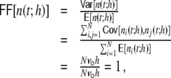
The average rate in all four networks is hardly affected by the underlying topology or weight distribution of the networks (cf. Table 1), while the variances of the population activity are very different. This is reflected in the respective Fano factors of population spike counts per time bin h = 0.1 ms, where is the number of spikes emitted by neuron i at time points s_l within the interval [t,t + h) (cf. Appendix A). If the population spike count n(t;h) is a compound process of independent stationary Poisson random variables n_i(t;h) with parameter , we have

9

because the covariances are zero for all i ≠ j and the variance of the sum equals the sum of the variances. If it is larger than one this indicates positive correlations between the spiking activities of the individual neurons (cf. Appendix A) (Papoulis 1991; Nawrot et al. 2008; Kriener et al. 2008). We see (cf. Table 1) that indeed it is largest for the Dale-conform ring network, still manifestly larger than one for the Dale-conform random network, and about one for the hybrid networks for both the ring and the random case. The quantitative differences of the Fano factors in all four cases can be explained by the different amount of pairwise spike train correlations (cf. Appendix A, Section 6). This demonstrates how a violation of Dale’s principle stabilizes and actually enables asynchronous irregular activity, even in networks whose adjacency, i.e. the mere unweighted connectivity, suggests highly correlated activity, as it is the case for Dale-conform ring (Fig. 2(a)) and small-world networks (Fig. 2(b)).

Table 1.

Mean population rates ν_o and Fano factors FF of population spike count n(t;h) per time bin h (10 s of population activity, N = 12,500, bin size h = 0.1 ms) for the random Dale and hybrid networks and the corresponding ring networks

Network type	Mean rate νo	Fano factor FF
Random, Dale	12.9 Hz	9.27
Random, Hybrid	12.8 Hz	1.25
Ring, Dale	13.5 Hz	26.4
Ring, Hybrid	13.1 Hz	1.13

If all spike trains contributing to the population spike count were uncorrelated Poissonian, the FF would equal 1. A FF larger than 1 indicates correlated activity (cf. Appendix A)

To understand the origin of the different correlation strengths in the various network types, and hence the different spiking dynamics and population activities in dependence on both the weight distribution and the rewiring probability, we will extend our analysis introduced in Kriener et al. (2008) to ring and small-world networks in the following sections.

Distance dependent correlations in a shot-noise framework

We assume that all incoming spike trains S_i(t) = ∑ _lδ(t − t_il) are realizations of point processes corresponding to stationary correlated Poisson processes, such that

10

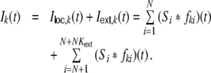
with spike train correlations c_ij ∈ [ − 1,1], and mean rates ν_i, ν_j (cf. however Fig. 4(d)). The spike trains can either stem from the pool of local neurons i ∈ {1,...,N} or from external neurons , where we assume that each neuron receives external inputs from neurons, which are different for all N local neurons. We describe the total synaptic input I_k(t) of a model neuron k as a sum of linearly filtered presynaptic spike trains (i.e. the spike trains are convolved with filter-kernels f_ki(t)), also called shot noise (Papoulis 1991; Kriener et al. 2008):

11

I_k(t) could represent e.g. the weighted input current, the synaptic input current (f_ki(t) = unit postsynaptic current, PSC), or the free membrane potential (f_ki(t) = unit postsynaptic potential, PSP). All synapses are identical in their kinetics and differ only in strength W_ki, hence we can write

12

With s_i(t): = (S_i ∗ f)(t), Eq. (11) is then rewritten as

13

The covariance function of the inputs I_k, I_l is given by

14

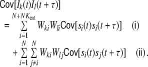
This sum can be split into

15

The first sum Eq. (15) (i) contains contributions of the auto-covariance functions of the filtered input spike trains, i.e. the spike trains that stem from common input neurons i ∈ {1,...,N} (W_kiW_li ≠ 0, including ). The second sum Eq. (15) (ii) contains all contributions of the cross-covariance functions of filtered spike trains that stem from presynaptic neurons i ≠ j, i,j ∈ {1,...,N}, where we already have taken into account that the external spike sources are uncorrelated, and hence for all . It is apparent that the high degree of shared input, as present in ring and small-world topologies, should show up in the spatial structure of input correlations between neurons. The closer two neurons k,l are located on the ring, the more common presynaptic neurons i they share. This will lead to a dominance of the first sum, unless the general strength of spike train covariances, accounted for in the second sum, is too high, and the second sum dominates the structural amplifications, because it contributes quadratically in neuron number. If the input covariances due to the structural overlap of presynaptic pools is however dominant, a fraction of this input correlation should also be present at the output side of the neurons, i.e. the spike train covariances c_ij should be a function of the interneuronal distance as well. This is indeed the case as we will see in the following.

Fig. 4.

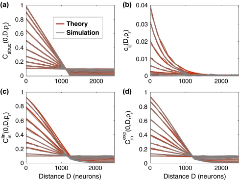
Input current (a, b, e) and spike train (c, f) correlation coefficients as a function of the pairwise interneuronal distance D for a ring network of size N = 12,500, κ = 1,250, g = 6, J = 0.1 mV with βN equidistantly distributed inhibitory neurons and external Poisson inputs per neuron of strength Hz each. (a) depicts the input correlation coefficients Eq. (18) derived with the assumption that the spike train correlation coefficients c_ij(D,0) go linearly like , cf. Eq. (30), and (b) fitted as a decaying exponential function (red). The gray curves show the input correlations estimated from simulations. (c) shows the spike train correlation coefficients estimated from simulations (gray), and both the linear (black) and exponential fit (red) used to obtain the theoretical predictions for the input correlation coefficients in (a) and (b). (d) shows the measured spike train cross-correlation functions ψ_ij(τ,D,0) for four different distances D = {1, 325, 625, 1250}. (e) shows the average input correlation coefficients (averaged over 50 neuron pairs per distance) and (f) the average spike train correlation coefficients measured in a hybrid ring network (for the full distribution cf. Fig. 7(c)). Note, that the average input correlations in (e) are even smaller than the spike train correlations in (c). For each network realization, we simulated the dynamics during 30 s. We then always averaged over 50 pairs for the input current correlations and 1,000 pairs for the spike train correlations with selected distances D ∈ {1, 10, 20,...,100, 200,..., 6,000}

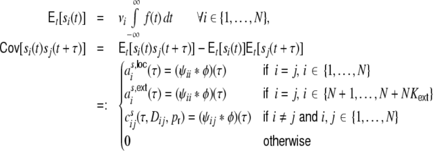
We will hence assume that all incoming spike train correlations c_ij are in general dependent on the pairwise distance D_ij = |i − j| of neurons i,j (neuron labeling across the ring in clockwise manner), and the rewiring probability . With Campbell’s theorem for shot noise (Papoulis 1991; Kriener et al. 2008) we can write

16

with

Here, represents the auto-correlation of the filter kernel f(t).

We now want to derive the zero time-lag input covariances, i.e. the auto-covariance and cross-covariance of I_k,I_l, defined as

17

in dependence of the auto- and cross-covariances , of the individual filtered input spike trains to obtain the input correlation coefficient

18

With the definitions Eq. (16) the input auto-covariance function at zero time lag , i.e. the variance of the input I_k, explicitly equals

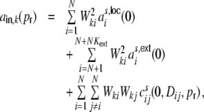19

while the cross-covariance of the input currents is given by

20

To assess the zero-lag shot noise covariances and we derive with Eqs. (10), (16)

21

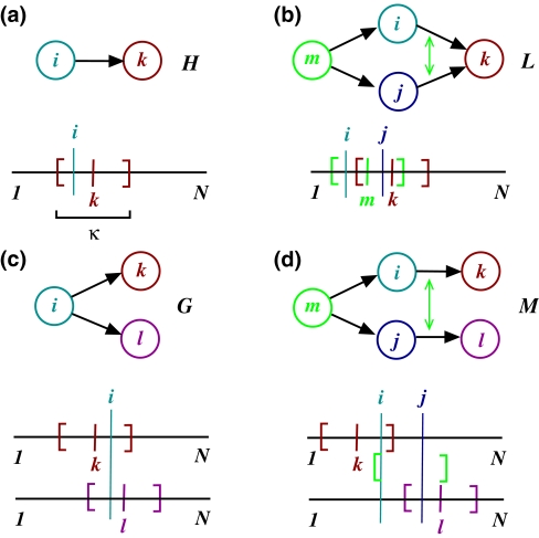
We assume for all i ∈ {1,...,N}, with denoting the average stationary rate of the network neurons, and for all , with denoting the rate of the external neurons. Hence, , and are the same for all neurons i ∈ {1,...,N}, and , respectively. For the cross-covariance function we analogously have . We define H_k as the contribution of the shot noise variances a^s to the variance of the inputs (cf. Fig. 3(a))

22

G_kl as the contribution of the shot noise variances a^s to the cross-covariance of the inputs (cf. Fig. 3(c))

23

L_k as the contribution of the shot noise cross-covariances c^s to the auto-covariance of the inputs (cf. Fig. 3(b))

24

and M_kl as the contribution of the shot noise cross-covariances c^s to the cross-covariance of the inputs (cf. Fig. 3(d))

25

Finally, if we assume input structure homogeneity, i.e. that the expected values of these individual contributions do not depend on k and l, but only on the relative distance D_kl and the rewiring probability , we can rewrite Eq. (18) as

26

The next two sections are devoted to the calculation of these expressions for ring and small-world networks.

Fig. 3.

Sketch of the different contributions to the input correlation coefficient , cf. Eq. (26) for the ring graph. The variance , Eq. (17) of the input to a neuron k is given by the sum of the variances H (panel (a)), Eq. (22) and the sum of the covariances L(0) (panel (b)), Eq. (24) of the incoming filtered spike trains s_i from neurons i ≠ j with W_kiW_kj ≠ 0. The cross-covariance , Eq. (17) is given by the sum of the variances of the commonly seen spike trains s_i with W_kiW_li ≠ 0, G(D_kl,0) (panel (c)), Eq. (23) and the sum of the covariances of the spike trains s_i from non-common input neurons i ≠ j with W_kiW_lj ≠ 0, M(D_kl,0), Eq. (25). We always assume that the only source of spike train correlations c_ij(D_ij,0) stems from presynaptic neurons sharing a common presynaptic neuron m (green)

Ring graphs

First we consider the case of Dale-conform ring networks, i.e. . A fraction of βκ of the presynaptic neurons i within the local input pool of neuron k is excitatory and depolarizes the postsynaptic neuron by W_ki = J with each spike, while (1 − β) κ presynaptic neurons are inhibitory and hyperpolarize the target neuron k by W_ki = − gJ per spike (cf. Section 2). Moreover, each neuron receives excitatory inputs from the external neuron pool with W_ki = J. Hence, for all neurons k ∈ {1,...,N} we obtain for the input variance H_k = H, Eq. (22), Fig. 3(a)

27

Because of the boxcar footprint, the contribution of the auto-covariances a^s(0) of the individual filtered spike trains to the input cross-covariance G_kl(D_kl,0), Eq. (23), is basically the same as H, only scaled by the respective overlap of the two presynaptic neuron pools of neurons k and l. This overlap only depends on the distance D_kl between k and l, cf. Fig. 3(c). Hence, for all k,l ∈ {1,...,N}

28

with minor modulations because of the exclusion of self-couplings and the relative position of the inhibitory neurons with respect to the boxcar footprint, but for large κ these corrections are negligible. Θ[x] is the Heaviside stepfunction that equals 1 if x ≥ 0, and 0 if x < 0. If all incoming spike trains from local neurons are uncorrelated and Poissonian, and the external drive is a direct current, the complete input covariance stems from the structural (i.e. common input) correlation coefficient alone, that can then be written as

29

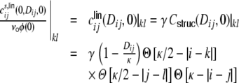
The spike train correlations c_ij(D_ij,0) show however a pronounced distance dependent decay and reach non-negligible amplitudes up to c_ij(1,0) ≈ 0.04 (cf. Fig. 4(c)). In the following we will use two approximations of the distance dependence of c_ij(D_ij,0), a linear relation and an exponential relation. We start by assuming a linear decay on the interval (0,κ] (cf. Fig. 4(c), black). This choice is motivated by two assumptions. First, we assume that the main source of spike correlations stems from the structural input correlations , Eq. (29), of the input neurons i,j alone, i.e. the strength of the correlations between two input spike trains S_i and S_j depends on the overlap of their presynaptic input pools, determined by their interneuronal distance D_ij. Analogous to the reasoning that lead to the common input correlations G(D_kl,0)/H, Eq. (29), before, the output spike train correlation between neurons i and j will hence be zero if D_ij ≥ κ. Moreover, the neurons i and j will only be contributing to the input currents of k and l, if they are within a distance κ/2, that is D_ki < κ/2 and D_lj < κ/2. Hence, for the correlations of two input spike trains S_i, S_j, i ≠ j to contribute to the input covariance of neurons k and l, these must be within a range κ + 2 κ/2 = 2κ. Additionally, we assume that the common input correlations are transmitted linearly with the same transmission gain to the output side of i and j. We hence make the following ansatz for the distance dependent correlations between the filtered input spike trains from neuron i to k and from neuron j to l (we always indicate the dependence on k and l by |_kl):

30

For the third sum in Eq. (19) this yields for all k ∈ {1,...,N} (cf. Appendix B for details of the derivation)

31

For the second term in Eq. (20) we have

32

which again only depends on the distance, so we dropped the sub-script of M. It is derived in Appendix B and explicitly given by Eq. (67). After calculation of and with the ansatz Eq. (30), we can plot as a function of distance and get a curve as shown in Fig. 4(a). It is obvious (Fig. 4(c)) that the linear fit overestimates the spike train correlations as a function of distance, the correlation transmission decreases with interneuronal distance, i.e. strength of input correlation , non-linearly (De la Rocha et al. 2007; Shea-Brown et al. 2008). This leads to an overestimation of the total input correlations for distances D_kl ≥ κ (Fig. 4(a)). If we instead fit the distance dependence of the spike train correlations of neuron i and j by a decaying exponential function with a cut-off at D_ij = κ,

33

and fit the corresponding parameters γ and η to the values estimated from the simulations, the sums in Eqs. (31) and (32) can still be reduced to simple terms (cf. Eqs. (69), (70)) and the correspondence with the observed input correlations becomes very good over the whole range of distances (Fig. 4(b)). We conclude that the strong common input correlations of neighboring neurons due to the structural properties of Dale-conform ring networks predominantly cause the spatio-temporally correlated spiking of neuron groups of size ∼κ.

However, we saw (cf. Fig. 2(d)) that the spiking activity in ring networks becomes highly asynchronous irregular, if we relax Dale’s principle and consider hybrid neurons instead. Since the number of excitatory, inhibitory and external synapses is the same for all neurons, we get the same expressions for H, and for hybrid neurons as well, but the common input correlations become (the expectation value is with regard to network realizations)

34

The ratio of and G hence corresponds to the one reported for random networks (Kriener et al. 2008) and equals 0.02 for the parameters used here. This is in line with the average input correlations in the hybrid ring network (Fig. 4(e)). They are hence only about half the correlation of the spike trains in the Dale-conform ring network (Fig. 4(c)). If we assume the correlation transmission for the highest possible input correlation to be the same as in the Dale case (γ ≈ 0.04), we estimate spike train correlations of the order of . The measured average values from simulations give indeed correlations of that range (Fig. 4(f)) and are, hence, of the same order as in hybrid random networks (Kriener et al. 2008). As we will show in Section 6, the distribution of input correlation coefficients is centered close to zero with a high peak at zero and both negative and positive contributions. In the Dale-conform ring network, however, we only observe positive correlation coefficients with values up to nearly one (it can only reach , if we apply identical external input to all neurons).

This transfers to the spike generation process and hence explains the dramatically different global spiking behavior, as well as the different Fano factors of the population spike counts (cf. Table 1, Appendix A) in both network types due to the decorrelation of common inputs in hybrid networks.

Small-world networks

As we stated before, the clustering coefficient (cf. Eq. (5)) is directly related to the amount of shared input between two neurons l and k, and hence to the strength of distance dependent correlations. When it gets close to the random graph value, as it is the case for , also the input correlations become similar to that of the corresponding balanced random network (cf. Fig. 5). If we randomize the network gradually by rewiring a fraction of connections, the input variance H is not affected. However, the input covariances due to common input do not only depend on the distance, but also on . The boxcar footprints of the ring network get diluted during rewiring, so a distance D_kl < κ does not imply anymore that all neurons within the overlap (κ − D_kl) of the two boxcars project to both or any of the neurons k,l (cf. Appendix B, Fig. 8(b)). At the same time the probability to receive inputs from neurons outside the boxcar increases during rewiring. These contributions are independent of the pairwise distance. Still, the probability for two neurons k,l with D_kl < κ to receive input from common neurons within the overlap of the (diluted) boxcars is always higher than the probability to get synapses from common neurons in the rest of the network, as long as : those input synapses that were not chosen for rewiring adhere to the boxcar footprint, and at the same time the boxcar regains a fraction of its synapses during the random rewiring. So, if D_kl < κ there are three different sources for common input to two neurons k and l that we have to account for: neurons within the overlap of input boxcars, that still have or re-established their synapses to k and l (possible in region ‘a’ in Fig. 8(b)), those that had not have any synapse to either k or l, but project to both k and l after rewiring (possible in region ‘c’ in Fig. 8(b)), and those that are in the boxcar footprint of one neuron k and got randomly rewired to another neuron outside of l’s boxcar footprint (possible in region ‘b’ in Fig. 8(b)). This implies that after rewiring neurons can be correlated due to common input in the regions ‘b’ and ‘c’, even if they are further apart than κ. These correlations due to the random rewiring alone are then independent of the distance between k and l. The probabilities for all these contributions to the total common input covariance are derived in detail in Appendix B. Ignoring the minor corrections due to the exclusion of self-couplings, we obtain for all k,l ∈ {1,...,N}

35

with (cf. Appendix B)

36

and

37

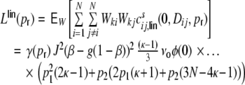
Since we always assume that the spike train correlations are caused solely by common input correlations transmitted to the output, i.e. that they are some function of , we also have to take this into account in the ansatz for the functional form of . Again, these spike train correlations lead to contributions to the cross-covariances of inputs I_k,I_l if D_kl < 2κ. With the linear distance dependence assumption we obtain (cf. Appendix B)

38

and for all k,l ∈ {1,...,N}

39

where we assumed that the rates, and the auto- and cross-covariances of the spike trains are the same for all neurons and neuron pairs, respectively. can be for evaluated as before. The same procedure as in the case hence gives the respective distance dependent input correlations (cf. Appendix B for details) for . The correspondence with the observed curves is good (Fig. 6). If we on the other hand apply cut-off exponential fits

40

of the distance dependent part of the spike train covariance functions, the shot noise covariance becomes

41

With this ansatz the correspondence of the predicted and measured input correlations is nearly perfect, as it was the case for the ring graphs (Fig. 6). For the random network the spike correlations c_ij(D_ij,1) are independent of distance and are proportional to the network connectivity ϵ (cf. also Kriener et al. (2008)), i.e. c_ij(D_ij,1) = ϵγ(1). This is indeed the case with the linear ansatz, as one can easily check with p₁(1) = p₂(1) = κ/N, cf. Eqs. (36), (37).

Fig. 5.

Clustering coefficient (black) versus the normalized input correlation coefficient (gray) estimated from simulations and evaluated at its maximum at distance D = 1 in a semi-log plot. decays slightly faster with than the clustering coefficient, but the overall shape is very similar. This shows how the topological properties translate to the joint second order statistics of neuronal inputs

Fig. 8.

Sketch how to derive the different contributions a, b, and c to the covariances in Eqs. (35), (39), (68), omitting the correction due to the non-existence of self-couplings. The ring is flattened-out and the left and right ends of each row are connected ((N + 1) = 1. (a) The ring network case : the neurons are in the center of their respective boxcar-neighborhoods of size κ marked in black. Black indicates a connection probability of 1, white indicates connection probability 0. The two neurons k and l > k are within a distance D_kl = |k − l| < κ from each other, hence they share common input from (κ − D_kl) neurons. The neurons k and l′, however, are farther apart than κ and do not have any common input neurons. (b) After rewiring, : The boxcar-neighborhood is diluted (dark-patterned) and the neurons have a certain probability to get input from outside the boxcar (light-patterned). Common input can now come in three different varieties: ‘a’, ‘b’ and ‘c’. If two neurons k, l are closer together than κ, the contribution of variety ‘a’ is proportional to the probability that a neuron within range still projects to both k and l after rewiring (cf. Eq. (61)). The contributions of variety ‘b’ are from neurons that projected to only one of both k or l before rewiring, but do now project to both k and l (cf. Eq. (62)). The contributions of the third variety ‘c’ are due to the number of common inputs proportional to the probability that neurons projected to neither k nor l in the original ring network, but do project to both after rewiring (cf. Eq. (63)). If two neurons k and l′ are farther apart than κ, they can have common input neurons after rewiring of varieties ‘b’ and ‘c’ only

Fig. 6.

Structural (a), spike train (b), and input (c, d) correlation coefficients as a function of the rewiring probability and the pairwise interneuronal distance D for a ring network of size N = 12,500, κ = 1,250, g = 6, J = 0.1 mV with βN equidistantly distributed inhibitory neurons and external Poisson inputs per neuron of strength Hz each. (a) The structural correlation coefficients . For they are close to one for D = 1 and tend to zero for D = 1,250. These would be the expected input correlation coefficients, if the spike train correlations were zero and the external input was DC. (b) shows the spike train correlations as estimated from simulations (gray) and the exponential fits (red) we used to calculate as shown in panel (d). (c) shows the input correlation coefficients (gray) estimated from simulations and the theoretical prediction (red) using linear fits of the respective . (d) shows the same as (c), but with fitted as decaying exponentials as shown in panel (c). For each network realization, we simulated the dynamics for 30 s. We then always averaged over 50 pairs for the input current correlations and 1,000 pairs for the spike train correlations with selected distances D ∈ {1, 10, 20,...,100, 200,..., 6000} and rewiring probabilities , always shown from top to bottom

With the spike train correlations fitted by an exponential, the correlation length actually diverges for , and Eq. (41) gives the wrong limit for D_kl < 2κ. As one can see in Fig. 6(b), the distance dependence of the spike correlations approaches a linear relation as the networks leave the small-world regime (), and the linear model becomes more adequate Eq. (30).

Distribution of correlation coefficients in ring and random networks

After derivation of the distance dependent correlation coefficients of the inputs in different neuronal network types, we can now ask for the distribution of correlation coefficients. In the following, we restrict the quantitative analysis to correlations of weighted input currents, but the qualitative results also hold for different linear synaptic filter kernels f_ki(t), cf. Section 5. Note that the mean structural input correlation coefficient is independent of ring or random topology, both in the Dale and the hybrid case, while the distributions differ dramatically (Fig. 7).

Fig. 7.

Estimated (gray) and predicted (red) input correlation coefficient probability density function (pdf) for a Dale-conform (a) ring and (b) random network, and for a hybrid (c) ring and (d) random network. (N = 12,500, κ = ϵN = 1,250, g = 6, estimation window size 0.005). The estimated data (gray) stem from 10s of simulated network activity and are compared with the structural input correlation probability mass functions in (b), (c), and (d) as derived in Eq. (46), Eq. (73), and Appendix D (red, binned with the same window as the simulated data), and compared to the full theory including spike correlations in (a, red). In (b), (c), and (d) the spike correlations are very small and hence close to the distributions predicted from the structural correlation (red). For the ring network, however, the real distribution differs substantially, due to the pronounced distance dependent spike train correlations. To obtain the full distribution in (a) and (c), we recorded from 6,250 subsequent neurons. Both have their maxima close to zero, we clipped the peaks to emphasize the less trivial parts of the distributions (the maximum of the pdf in (a) is 142 in theory and 136 in the estimated distribution; the maximum of the pdf in (b) is 160 in theory and 156 in the estimated distribution). For the random networks (b, d), we computed all pairwise input correlations of a random sample of 50 neurons. The oscillations of the analytically derived pdf in (b, red) are due to the specific discrete nature of the problem, cf. Eq. (46)

Ring networks

42

with the distribution of pairwise distances ,3 and

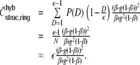43

Random networks (Kriener et al. 2008)

44

and

45

where (1 − β) and β are the fractions of inhibitory and excitatory inputs per neuron (each the same for all neurons).

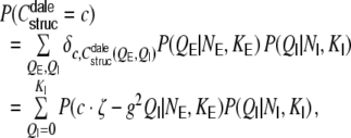
The distribution of structural correlation coefficients in the random Dale network is given by

46

where , is the number of common inhibitory inputs and that of excitatory ones,

47

and

48

Note that for non-integer . The correlation coefficient distribution for the random hybrid network is derived in Appendix D.

For a ring graph the structural correlation coefficient distribution has the probability mass at the origin, in the discrete open interval (0,1), and at 1, if we include the variance for distance D = 0. However, due to the non-negligible spike train correlations c_ij(D,0), the actually measured input correlations have a considerably different distribution that has less mass at 0 due to the positive input correlations up to a distance ∼2κ. They are very well described by the full theory with an exponential ansatz for the spike train correlations as described in Section 5.1, Eq. (41). These two limiting cases emphasize that the distribution of input (subthreshold) correlations may give valuable information about whether there is a high degree of locally shared input (heavy tail probability distribution ) or if it is rather what is to be expected from random connectivity in a Dale-conform network.

Discussion

We analyzed the activity dynamics in sparse neuronal networks with ring, small-world and random topologies. In networks with a high clustering coefficient such as ring and small-world networks, neighboring neurons tend to fire highly synchronously. With increasing randomness, governed by the rewiring probability , activity becomes more asynchronous, but even in random networks we observe a high Fano factor FF of the population spike counts, indicating its residual synchrony.4 As shown by Kriener et al. (2008) these fluctuations become strongly attenuated for hybrid neurons which have both excitatory and inhibitory synaptic projections.

Here, we demonstrated that the introduction of hybrid neurons leads to highly asynchronous (FF ≈ 1) population activity even in networks with ring topology. Recent experimental data suggest, that there are abundant fast and reliable couplings between pyramidal cells, which are effectively inhibitory (Ren et al. 2007) and which might be intepreted as hybrid-like couplings. However, the hybrid concept contradicts the general paradigm that pyramidal cells depolarize all their postsynaptic targets while inhibitory interneurons hyperpolarize them, a paradigm known as Dale′sprinciple (Li and Dayan 1999; Dayan and Abbott 2001; Hoppensteadt and Izhikevich 1997). As we showed here, a severe violation of Dale’s principle turns the specifics of network topology meaningless, and might even impede functionally potentially important processes, as for example pattern formation or line attractors in ring networks (see e.g. Ben-Yishai et al. 1995; Ermentrout and Cowan 1979), or propagation of synchronous activity in recurrent cortical networks (Kumar et al. 2008a).

We demonstrated that the difference of the amplitude of population activity fluctuations in Dale-conform and hybrid networks can be understood from the differences in the input correlation structure in both network types. We extended the ansatz presented in Kriener et al. (2008) to networks with ring and small-world topology and derived the input correlations in dependence of the pairwise distance of neurons and the rewiring probability. Because of the strong overlap of the input pools of neighboring neurons in ring and small-world networks, the assumption that the spike trains of different neurons are uncorrelated, an assumption justified in sparse balanced random networks, is no longer valid. We fitted the distance dependent instantaneous spike train correlations and took them adequately into account. This lead to a highly accurate prediction of input correlations.

A fully self-consistent treatment of correlations is however beyond the scope of the analysis presented here. As we saw in Section 5.1, in Dale-conform ring graphs neurons cover basically the whole spectrum of positive input correlation strengths between almost one (depending on the level of variance of the uncorrelated external input) and zero as a function of pairwise distance D. If we look at the ratio between input and output correlation strength, we see that it is not constant, but that stronger correlations have a higher gain. The exact mechanisms of this non-linear correlation transmission needs further analysis. Recent analysis of correlation transfer in integrate-and-fire neurons by De la Rocha et al. (2007) and Shea-Brown et al. (2008) showed that the spike train correlations can be written as a linear function of the input correlations, given they are small . For larger (De la Rocha et al. 2007; Shea-Brown et al. 2008), however, report supralinear correlation transmission. Such correlation transmission properties were also observed and analytically derived for arbitrary input correlation strength in an alternative approach that makes use of correlated Gauss processes (Tchumatchenko et al. 2008). These results are all in line with the non-linear dependence of spike train correlations on the strength of input correlations that we observed and fitted by an exponential decay with interneuronal distance.

We saw that correlations are weakened as they are transferred to the output side of the neurons, but, as is to be expected, they are much higher for neighboring neurons in ring networks as it is the case in the homogeneously correlated random networks that receive more or less uncorrelated external inputs. The assumption that the spike train covariance functions are delta-shaped is certainly an over-simplification, especially in the Dale-conform ring networks (cf. the examples of spike train cross-correlation functions ψ_ij(τ,D,0), Fig. 4(d)). The temporal width of the covariance functions leads to an increase in the estimation of spike train correlations if the spike count bin-size h is increased. In Dale-conform ring graphs we found c_ij(1,0) ≤ 0.041 for time bins h = 0.1 ms (cf. Fig. 4(c), (d)). For h = 10 ms, a time window of the order of the membrane time constant , we observed c_ij(1,0) ≤ 0.25 (not shown). This covers the spectrum of correlations reported in experimental studies, which range from 0.01 to approximately 0.3 (Zohary et al. 1994; Vaadia et al. 1995; Shadlen and Newsome 1998; Bair et al. 2001). For hybrid networks, however, the pairwise correlations have a narrow distribution around zero, irrespective of the topology. This explains the highly asynchronous dynamics in hybrid neuronal networks.

Finally, we suggest that the distribution of pairwise correlation coefficients of randomly chosen intracellularly recorded neurons may provide a means to distinguish different neuronal network topologies. Real neurons, however, have conductance-based synapses, and their filtering is strongly dependent on the membrane depolarization (Destexhe et al. 2003; Kuhn et al. 2004). Moreover, spikes are temporally extended events, usually with different synaptic time scales, and transmission delays are distributed and likely dependent on the distance between neurons. These effects, amongst others, might distort the results presented here. Still, though intracellular recordings are technically more involved than extracellular recordings, they are basically analog signals, and hence much shorter periods of recording time are necessary to get a sufficiently good statistics, as compared to estimation of pairwise spike train correlations from low rate spiking neurons (Lee et al. 2006). So, bell-shaped distributions of membrane potential correlations may hint towards an underlying random network structure, while heavy-tail distributions should be observed for networks with locally confined neighborhoods. Naturally, the distribution will depend on the relation between the sampled region and the footprint of the neuron-type one is interested in. This is true for both the model as well as for real neuronal tissue. Some idea about the potential input footprint, e.g. from reconstructions of the axonal and dendritic arbors (Hellwig 2000; Stepanyants et al. 2007), can help to estimate the spatial distance that must be covered. It also is a matter of the spatial scale that one is interested in: if one is mostly interested in very small, local networks < 200 μm, where the connection probability might be considered approximately homogeneous (Hellwig 2000; Stepanyants et al. 2007), the correlation coefficient distribution will be akin to that of a random topology. If one, however, samples several millimeter, the distribution may tend more to a heavy-tail shape, due to the increase of the relative number of weakly correlated neuron pairs. At this scale radial inhomogeneities, as for example due to axonal patches (Lund et al. 2003), in two dimensions or different connection probabilities within and between cortical layers (Binzegger et al. 2004) in three dimensions must be taken into account as well, as they will distort the over-simplified assumption of the connectivity made here. In conclusion, we think that a further extension of the line of research presented here might provide a way to access structural features of neuronal networks by the analysis of their input statistics. This could eventually prove helpful in separating correlations that arise due to the specifics of the network structure from those that arise due to correlated input from other areas, e.g. sensory inputs, and provide insight into the relation between structure and function.

Appendix A: Fano factor

In this appendix we want to quantitatively formulate the Fano factor FF[n(t;h)] of spike counts n(t;h) per time bin h. We assume that the compound spike train, i.e. the population activity is an ensemble of Poisson point processes. The population spike count with regard to a certain time bin h is then a sum of random variables (Papoulis 1991) defined by

49

The expectation value is given by (exploiting the linearity of the expectation value):

50

is generally given by (Papoulis 1991; Nawrot et al. 2008)

51

For stationary Poisson processes with intensity ν, we have mean and variance

52

Hence , provided all processes are independent. If we have homogeneously correlated Poisson processes (cf. Eq. (10)), such that for all i,j ∈ {1,...,N} , the variance of the population count is given by

53

For the Fano factor we hence obtain . For homogeneously correlated networks like random networks this estimate is indeed very close to the actually measured FF (Kriener et al. 2008). For the ring and small-world networks we have in Eq. (53), since the spike count estimation is a linear filtering and hence Campbell’s theorem Eq. (16) can be applied. For the Dale-conform ring network , yielding a . The FF estimated from simulations is indeed of that order, cf. Table 1.

Appendix B: Distance dependent correlations—linear fit

To estimate the contributions to the covariances in Eqs. (35), (39), (68) in detail for we first calculate the distribution of non-zero entries in each matrix row in dependence of . If we remove exactly (incoming) synapses from the boxcar neighborhood of a neuron and randomly redraw them (without establishing multiple and self-connections) from the possible presynaptic neurons, the distribution for reestablishing q connections that were there before is given by

54

and that of establishing r new connections is

55

In expectation we hence have

56

connections from within the ring boxcar neighborhood κ, and

57

new connections from outside the boxcar neighborhood.5 We then define the probability of a neuron within the boxcar neighborhood and the probability of a neuron outside the boxcar neighborhood to project to a neuron k, k ∈ {1,...,N} by

58

and

59

With the notation from Fig. 8 we get the expected number

60

of common inputs Q to neuron k and neuron l in dependence of D_kl and with

61

62

and

63

For two neurons k and l we assumed (cf. Eq. (38)) the spike train correlations between input neuron i of k and input neuron j of l to be given by

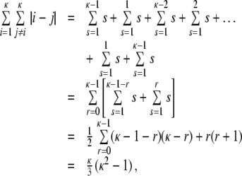
The double-sum over all pairwise distances D_ij = |i − j| can be expressed by a simple summation formula:

64

and hence we can evaluate with Defs. (61), (62), (63) and :

65

We assume k ≠ l and, without loss of generality, k > l. We set D_kl = |k − l| = (k − l): = d and we always omit the explicit modulo-notation due to periodic boundary conditions. For we calculate

66

We define the alias

and obtain:

We can evaluate the Heaviside step-functions and rewrite the sums as

where the cases occur due to the negligence of k,l in the summation and we need to subtract the over- counted terms i = j. A shift of the summation indices yields:

Now we perform a similar, but more involved resorting as in Eq. (64) and split the sum into various contributions that correspond to the same boundary conditions:

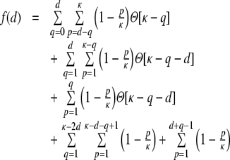We have to keep in mind that d ∈ {1,...,2κ}. Hence, e.g. the first term in the latter identity

has two distance-regimes, one where κ ≥ d and the stepfunction is always one, and the second, where κ < d ≤ 2κ, and the stepfunction truncates all summands with q > κ. This has to be taken into account when calculating the summation formula:

where in the first identity we used the stepfunction, and have to keep in mind that all summands in the inner sum with a lower summation index exceeding the upper one are zero, hence , i.e. . In the second identity we performed a simple index shift operation. After we evaluated the stepfunctions, it is straightforward to find the corresponding summation formulae (Bronstein and Semendjajew 1987):

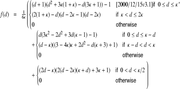67

(*) The minus one contribution comes about by correcting for the omission of neurons k and l during summation over the κ neighbors.

In general we numerically evaluated:

68

Appendix C: Distance dependent correlations—exponential fit

With the ansatz Eq. (38)

we obtain analogously to the linear case Appendix B, Eq. (39)

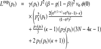69

and for :

70

We once more omit the explicit modulo-notation due to periodic boundary conditions and obtain analogously to the linear case, Appendix B:

71

(*) The minus contribution comes about by correcting for the omission of neurons k and l during summation over the κ neighbors.

In general we numerically evaluated:

72

Appendix D: Distribution of correlation coefficients in the hybrid ring and random network

In the hybrid random network case we get a distribution

73

for the distribution of the number of total common inputs Q. κ is the total number of input synapses per neuron. Given that common input pool of size Q, we then ask for the probability to have n_i + incoming excitatory synapses to neuron N_i and n_j + incoming excitatory synapses to neuron N_j. We have

74

If we, moreover, know n_+ +, i.e. the number of incoming synapses from Q that are excitatory for both N_i and N_j, we know the residual possible combinations of signs (cf. Fig. 9). n_+ + follows the probability distribution

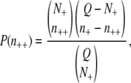75

with and . We get

76

Fig. 9.

Sketch how to derive n_− +, n_+ − and n_− −, given n_i +, n_j + and n_+ +

Hence, the correlation coefficient given n_i +, n_j + and n_+ + yields ()

77

The probability distribution is then given by

78

The hybrid ring case is obtained analogously by taking into account that all nontrivial overlaps Q ∈ {1,...,κ − 1} occur exactly twice, hence the probability P(Q) for all possible non-trivial Q is 2/(N − 1). Additionally, there are (N − 2κ − 1) possible neuron pairs drawn with probability 1/(N − 1) that do not share common input and are hence zero.

References

- Albert, R., & Barabasi, A. (2002). Statistical mechanics of complex networks. Reviews of Modern Physics, 74, 47–97. [DOI]
- Bair, W., Zohary, E., & Newsome, W. (2001). Correlated firing in Macaque visual area MT: Time scales and relationship to behavior. Journal of Neuroscience, 21(5), 1676–1697. [DOI] [PMC free article] [PubMed]
- Ben-Yishai, R., Bar-Or, R., & Sompolinsky, H. (1995). Theory of orientation tuning in visual cortex. Proceedings of the National Academy of Sciences of the United States of America, 92, 3844. [DOI] [PMC free article] [PubMed]
- Binzegger, T., Douglas, R. J., & Martin, K. A. C. (2004). A quantitative map of the circuit of cat primary visual cortex. Journal of Neuroscience, 39(24), 8441–8453. [DOI] [PMC free article] [PubMed]
- Bronstein, I. N., & Semendjajew, K. A. (1987). Taschenbuch der Mathematik (23rd ed.). Thun und Frankfurt/Main: Verlag Harri Deutsch.
- Brunel, N. (2000). Dynamics of sparsely connected networks of excitatory and inhibitory spiking neurons. Journal of Computational Neuroscience, 8(3), 183–208. [DOI] [PubMed]
- Brunel, N., & Hakim, V. (1999). Fast global oscillations in networks of integrate-and-fire neurons with low firing rates. Neural Computation, 11(7), 1621–1671. [DOI] [PubMed]
- Chklovskii, D. B., Schikorski, T., & Stevens, C. F. (2002). Wiring optimization in cortical circuits. Neuron, 34, 341–347. [DOI] [PubMed]
- Dayan, P., & Abbott, L. F. (2001). Theoretical neuroscience. Cambridge: MIT.
- De la Rocha, J., Doiron, B., Shea-Brown, E., Kresimir, J., & Reyes, A. (2007). Correlation between neural spike trains increases with firing rate. Nature, 448(16), 802–807. [DOI] [PubMed]
- Destexhe, A., Rudolph, M., & Pare, D. (2003). The high-conductance state of neocortical neurons in vivo. Nature Reviews. Neuroscience, 4, 739–751. [DOI] [PubMed]
- Ermentrout, G. B., & Cowan, J. D. (1979). A mathematical theory of visual hallucination patterns. Biological Cybernetics, 34, 137–150. [DOI] [PubMed]
- Gewaltig, M.-O., & Diesmann, M. (2007). NEST (Neural simulation tool). Scholarpedia, 2(4), 1430.
- Hellwig, B. (2000). A quantitative analysis of the local connectivity between pyramidal neurons in layers 2/3 of the rat visual cortex. Biological Cybernetics, 2(82), 111–121. [DOI] [PubMed]
- Hoppensteadt, F. C., & Izhikevich, E. M. (1997). Weakly connected neural networks. New York: Springer.
- Jahnke, S., Memmesheimer, R., & Timme, M. (2008). Stable irregular dynamics in complex neural networks. Physical Review Letters, 100, 048102. [DOI] [PubMed]
- Kriener, B., Tetzlaff, T., Aertsen, A., Diesmann, M., & Rotter, S. (2008). Correlations and population dynamics in cortical networks. Neural Computation, 20, 2185–2226. [DOI] [PubMed]
- Kuhn, A., Aertsen, A., & Rotter, S. (2004). Neuronal integration of synaptic input in the fluctuation-driven regime. Journal of Neuroscience, 24(10), 2345–2356. [DOI] [PMC free article] [PubMed]
- Kumar, A., Rotter, S., & Aertsen, A. (2008a). Conditions for propagating synchronous spiking and asynchronous firing rates in a cortical network model. Journal of Neuroscience, 28(20), 5268–5280. [DOI] [PMC free article] [PubMed]
- Kumar, A., Schrader, S., Aertsen, A., & Rotter, S. (2008b). The high-conductance state of cortical networks. Neural Computation, 20(1), 1–43. [DOI] [PubMed]
- Lee, A., Manns, I., Sakmann, B., & Brecht, M. (2006). Whole-cell recordings in freely moving rats. Neuron, 51, 399–407. [DOI] [PubMed]
- Li, Z., & Dayan, P. (1999). Computational differences between asymmetrical and symmetrical networks. Network: Computing Neural Systems, 10, 59–77. [DOI] [PubMed]
- Lund, J. S., Angelucci, A., & Bressloff, P. C. (2003). Anatomical substrates for functional columns in macaque monkey primary visual cortex. Cerebral Cortex, 12, 15–24. [DOI] [PubMed]
- Mattia, M., & Del Guidice, P. (2002). Population dynamics of interacting spiking neurons. Physical Review E, 66, 051917. [DOI] [PubMed]
- Mattia, M., & Del Guidice, P. (2004). Finite-size dynamics of inhibitory and excitatory interacting spiking neurons. Physical Review E, 70, 052903. [DOI] [PubMed]
- Morrison, A., Mehring, C., Geisel, T., Aertsen, A., & Diesmann, M. (2005). Advancing the boundaries of high connectivity network simulation with distributed computing. Neural Computation, 17(8), 1776–1801. [DOI] [PubMed]
- Nawrot, M. P., Boucsein, C., Rodriguez Molina, V., Riehle, A., Aertsen, A., & Rotter, S. (2008). Measurement of variability dynamics in cortical spike trains. Journal of Neuroscience Methods, 169, 374–390. [DOI] [PubMed]
- Papoulis, A. (1991). Probability, random variables, and stochastic processes (3rd ed.). Boston: McGraw-Hill.
- Ren, M., Yoshimura, Y., Takada, N., Horibe, S., & Komatsu, Y. (2007). Specialized inhibitory synaptic actions between nearby neocortical pyramidal neurons. Science, 316, 758–761. [DOI] [PubMed]
- Shadlen, M. N., & Newsome, W. T. (1998). The variable discharge of cortical neurons: Implications for connectivity, computation, and information coding. Journal of Neuroscience, 18(10), 3870–3896. [DOI] [PMC free article] [PubMed]
- Shea-Brown, E., Josic, K., de la Rocha, J., & Doiron, B. (2008). Correlation and synchrony transfer in integrate-and-fire neurons: Basic properties and consequences for coding. Physical Review Letters, 100, 108102. [DOI] [PubMed]
- Song, S., Per, S., Reigl, M., Nelson, S., & Chklovskii, D. (2005). Highly nonrandom features of synaptic connectivity in local cortical circuits. Public Library of Science, Biology, 3(3), 0507–0519. [DOI] [PMC free article] [PubMed]
- Sporns, O. (2003). Network analysis, complexity and brain function. Complexity, 8(1), 56–60. [DOI]
- Sporns, O., & Zwi, D. Z. (2004). The small world of the cerebral cortex. Neuroinformatics, 2, 145–162. [DOI] [PubMed]
- Stepanyants, A., Hirsch, J., Martinez, L. M., Kisvarday, Z. F., Ferecsko, A. S., & Chklovskii, D. B. (2007). Local potential connectivity in cat primary visual cortex. Cerebral Cortex, 18(1), 13–28. [DOI] [PubMed]
- Strogatz, S. H. (2001). Exploring complex networks. Nature, 410, 268–276. [DOI] [PubMed]
- Tchumatchenko, T., Malyshev, A., Geisel, T., Volgushev, M., & Wolf, F. (2008). Correlations and synchrony in threshold neuron models. http://arxiv.org/pdf/0810.2901. [DOI] [PubMed]
- Tetzlaff, T., Rotter, S., Stark, E., Abeles, M., Aertsen, A., & Diesmann, M. (2007). Dependence of neuronal correlations on filter characteristics and marginal spike-train statistics. Neural Computation, 20, 2133–2184. [DOI] [PubMed]
- Timme, M. (2007). Revealing network connectivity from response dynamics. Physical Review Letters, 98, 224101. [DOI] [PubMed]
- Timme, M., Wolf, F., & Geisel, T. (2002). Coexistence of regular and irregular dynamics in complex networks of pulse-coupled oscillators. Physical Review Letters, 89(25), 258701. [DOI] [PubMed]
- Vaadia, E., Haalman, I., Abeles, M., Bergman, H., Prut, Y., Slovin, H., & Aertsen, A. (1995). Dynamics of neuronal interactions in monkey cortex in relation to behavioural events. Nature, 373(6514), 515–518. [DOI] [PubMed]
- van Vreeswijk, C., & Sompolinsky, H. (1996). Chaos in neuronal networks with balanced excitatory and inhibitory activity. Science, 274, 1724–1726. [DOI] [PubMed]
- van Vreeswijk, C., & Sompolinsky, H. (1998). Chaotic balanced state in a model of cortical circuits. Neural Computation, 10, 1321–1371. [DOI] [PubMed]
- Watts, D. J., & Strogatz, S. H. (1998). Collective dynamics of small-world networks. Nature, 393, 440–442. [DOI] [PubMed]
- Yoshimura, Y., & Callaway, E. (2005). Fine-scale specificity of cortical networks depends on inhibitory cell type and connectivity. Nature Neuroscience, 8(11), 1552–1559. [DOI] [PubMed]
- Yoshimura, Y., Dantzker, J., & Callaway, E. (2005). Excitatory cortical neurons form fine-scale functional networks. Nature, 433(24), 868–873. [DOI] [PubMed]
- Zohary, E., Shadlen, M. N., & Newsome, W. T. (1994). Correlated neuronal discharge rate and its implications for psychophysical performance. Nature, 370, 140–143. [DOI] [PubMed]