

Abstract
As the use of effective connectivity as become more popular, it is important to understand how the results from different analyses compare with each other, as the results from studies employing differing methods for determining connectivity may not reach the same conclusion. Simulated fMRI time series data were used to compare the results from four of the more commonly used computational methods, structural equation modeling, autoregressive analysis, Granger causality, and dynamic causal modeling to determine which may be better suited to the task. The results show that all three methods are able to detect changes in system dynamics. Structural equation modeling appeared to be the least sensitive to changes in TR or source of variance, and Granger causality the most sensitive. The results also suggest that improved reporting on data analyses is necessary, and employing an effect statistic to depict results may remove some of the ambiguity in comparing results across studies using differing methods to determine connectivity.
Keywords: Keywords Effective connectivity, Structural equation modeling, Autoregressive analysis, Granger causality, Dynamic causal modeling, Sources of variance
Introduction
The use of effective connectivity has become more popular, with no single method being used to the exclusion of others. This poses problems when attempting to compare results across studies, as the multiple ways in which connectivity can be determined will not necessarily lead to the same conclusion about whether two or more neural units are strongly interacting or not (Horwitz 2003). Several different models including structural equation modeling (McIntosh and Gonzalez-Lima 1994; Buchel and Friston 1997), nonlinear system identification techniques (Friston and Buchel 2000), autoregressive techniques (Harrison et al. 2003; Goebel et al. 2003; Roebroeck et al. 2005), and dynamic causal modeling (Friston et al. 2003) have been introduced as valid methods for estimating effective connectivity from fMRI time series data. Additionally, several methods for correlating the data have been introduced including across (Bullmore et al. 2000) or within (Hampson et al. 2002) conditions, across (Bokde et al. 2001) or within (Goncalves et al. 2001) subjects, or some combination of these. As these computational methods and data modeling techniques can be combined in many ways, it is important to understand how the results from these different pairings compare with each other and if any of the pairings may be better suited to calculating effective connectivity from fMRI data than the others.
Structural equation modeling (SEM) has been applied to fMRI data from a wide variety of neural systems (Buchel and Friston 1997; Grafton et al. 1994; Maguire 2001; McIntosh and Gonzalez-Lima 1994; Zhuang et al. 2005). However, several papers have outlined drawbacks of applying SEM to fMRI data (Buchel and Friston 1997; Penny et al. 2004; Harrison et al. 2003; Yamashita 2005; Ramnani 2004), with two of the more commonly cited being its requirement of an a priori anatomical model of regions and directed paths and its assumption of instantaneous connections. Autoregressive analysis (AR) has been proposed as an alternative method for calculating effective connectivity, as it does not share the same drawbacks as SEM (Harrison et al. 2003). Namely, it does not require an a priori anatomical model, and it is able to take in account the rich temporal information inherent in fMRI data. More recently, Granger causality has been used as a summary measure of the results obtained from AR analyses, growing in popularity in part because it allows the results to be mapped on to the brain much like fMRI results (Goebel et al. 2003; Roebroeck et al. 2005). One potential drawback of Granger causality may be that the temporal resolution of the standard fMRI experiment may be too low for it to provide a complete picture of the dynamics of the neural system of interest. While the use of Granger causality is increasing, neither it nor AR analysis have enjoyed the same popularity as SEM, having been applied to only a handful of neural systems (Harrison et al. 2003; Goebel et al. 2003; Roebroeck et al. 2005).
Dynamic causal modeling (DCM) can be distinguished from the three methods described above in that it was designed specifically to accommodate fMRI time series data. DCM aims to treat the brain as a deterministic nonlinear system that is subject to inputs and produces outputs. Connectivity is described in terms of the coupling among unobserved brain states, or the neuronal activity within different brain regions. Connectivity can be determined by perturbing the system, such as through the presentation of a stimulus, and measuring the response. In addition to its inclusion of the Balloon model, DCM can be distinguished from the above three computational methods by accommodating the nonlinear and dynamic aspects of neuronal interactions, as well as allowing the estimation process to include experimentally designed inputs (Friston et al. 2003).
Structural equation modeling (SEM) (McIntosh and Gonzalez-Lima 1994), autoregressive analysis (AR) (Harrison et al. 2003), Granger causality (Goebel et al. 2003; Roebroeck et al. 2005), and dynamic causal modeling (DCM) (Friston et al. 2003) have emerged as four of the more popular methods from which to calculate effective connectivity from fMRI time series data. The common feature among these four methods is their estimation of correlation and covariance matrices, meaning the results will, in part, depend on the sources of variance used (Caclin and Fonlupt 2006; Horwitz et al. 2005). For fMRI-based experiments, this underlying variance is more often temporal in nature—a function of the deviation of a repeated measurement with a subject across time. This temporal variance, additionally, can be task-related or intrinsic in nature (Rogers et al. 2007).
For a standard block-design involving more than one experimental condition, within-subject task-related variance takes into account the complete, undoctored time series, assuming that the connectivity is constant across all experimental conditions. The effective connectivity measured, then, is the average connectivity during all conditions. In contrast to task-related variance that takes advantage of changes in the fMRI signal that are directly related to changes in experimental stimuli across acquisitions, intrinsic variance is not the result of any specific stimulus. Rather, fluctuations in the BOLD signal act as the neurophysiological index reflecting common neural activity across different brain regions (Rogers et al. 2007). The ideal method to measure connectivity from the intrinsic variance in the BOLD signal would be to have the task of interest performed in a steady-state manner—performed constantly and consistently throughout the data acquisition window. The use of steady-state task performance attempts to minimize the variance introduced by individual trial-to-trial performance of the task itself. Practically, however, for a standard block design, intrinsic variance may be utilized by either trimming the time series to keep only those volumes scanned during the condition of interest (Honey et al. 2002; Bokde et al. 2001; Homae et al. 2003), to create what will be referred to as a trimmed time series, or by using the entire time series after removing any task-related components by some means such as independent component analysis (Arfanakis et al. 2000) or linear regression (Rogers et al. 2007).
As stated above, Horwitz (2003) pointed out that there is still no consensus as to a single computational method for estimating effective connectivity from fMRI data, posing problems when comparing results across studies using differing computational methods and sources of variance. To this end, the results from the above mentioned methods—structural equation modeling, autoregressive analysis, Granger causality, and dynamic causal modeling—have been compared using simulated fMRI time series data with known, modeled connectivity to determine if any of these methods holds a distinct advantage over the others.
Theory
This section is not meant to be a comprehensive review of the theories underlying the various computational methods being considered in this investigation. Rather, it is meant to provide a brief overview of the equations involved. The authors refer the readers to the respective papers for further discussion of the specific methods.
Structural equation modeling
Structural equation modeling works by extracting information about neural interactions through the decomposition of interregional covariances of activity. The measure of covariance between two neural elements represents the degree to which the activity of these two elements is related to one another, or how they vary together (McIntosh and Gonzalez-Lima 1994). The relationship between brain regions can be described using a simple linear mathematical of the variance of a region as influenced by the variance of another.
| (1) |
In the above equation, Y and X are the regional time series, with the beta term being the path weight. Alpha represents the y-intercept, which can easily be set to zero. Psi is the residual term.
Autoregressive analysis
For linear autoregressive models, given a multivariate system, one can model the current value of a regional time series as a weighted linear sum of the previous value of another regional time series (Harrison et al. 2003).
| (2) |
Y and X represent the regional time series in the above equation. The path weights are contained in the vector A and the residuals in the vector e. Finally, p represents the order of the model.
Granger causality
Granger causality quantifies the usefulness of unique information in one time series in predicting the values of a second time series. Given two time series, X[n] and Y[n], if incorporating past values of X improves the prediction of the current value of Y, then one can say that X Granger causes Y (Goebel et al. 2003; Roebroeck et al. 2005). Geweke (1982, 1984) proposed a measure of linear dependence, which implements Granger causality in terms of vector autoregressive models. In this framework, Geweke defined this measure of linear dependence as
| (3) |
In the above equation, the term to the left of the equal sign is the total linear dependence of regional time series X and Y. The path weight information is contained in the directed linear dependence terms between X and Y, the first two terms to the right of the equal sign. The final term in the above equation represents the instantaneous influence between X and Y and, for the purposes of fMRI-based connectivity studies, contains any linear dependence between the two time series that occurs on a time scale to small for fMRI to measure (Roebroeck et al. 2005).
The dependence measures shown above can be defined using the autocorrelation matrices of the residuals of the following three vector autoregressive models, where the autocorrelation matrices of the residuals are given by Sigma, Tau, and Upsilon.
| (4.A) |
| (4.B) |
| (4.C) |
The residual correlation matrices, in turn, quantify how well one is able to predict current values of regional time series from their past values. From these residual correlation matrices, one can define Geweke’s linear dependence terms as
| (5.A) |
| (5.B) |
| (5.C) |
| (5.D) |
Dynamic causal modeling
Dynamic causal models (Friston et al. 2003) consist of a bilinear model, which includes both neurodynamics and an extended Balloon model (Friston 2002; Buxton et al. 1998). The neurodynamics can be described by a multivariate differential equation.
| (6) |
The variable t indexes continuous time, and the dot denotes a time derivative. The path weights, or effective connectivity, are described by a set of intrinsic connections and contained within the variable A. Modulatory and input connections are specified in Bj and C, respectively.
Methods
Simulated data
Functional MRI time series were simulated using the dynamic causal modeling (DCM) simulation code supplied with SPM2 (Wellcome Department of Cognitive Neurology, London, UK). The DCM simulator was employed as a convenient way to create simulated fMRI time series data with known, modeled connectivity that is, for the purposes of this investigation, unbiased towards three of the methods under consideration. A simple, three-region DCM system with three unidirectional intrinsic connections, as shown in Fig. 1, was modeled. The intrinsic connection between Regions 1 and 2 was varied as I={0.1, 0.2, 0.3, 0.4, 0.5, 0.6, 0.7, 0.8, 0.9}. An fMRI experiment was applied as an extrinsic connection to Region 1 with a constant weight of 0.7. The remaining two connections between Regions 1 and 3 and Regions 3 and 2 were held at a constant value of 0.1.
Fig. 1.
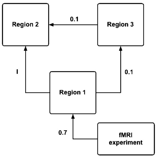
Path model (causal structure) used to guide the time series simulations. The path from Region 1 to Region 2 was varied I={0.1, 0.2, 0.3, 0.4, 0.5, 0.6, 0.7, 0.8, 0.9}. The strengths of the fMRI experiment and the remaining two paths were held constant at the values indicated
In addition to varying the intrinsic path weight, two separate fMRI experiments were used to take into consideration the two sources of variance described in the introduction, task-related and intrinsic. For both the time series simulated to include task-related variance (Fig. 2a) and intrinsic variance for the trimmed case (Fig. 2c), a standard block design consisting of alternating 20-second blocks of ‘rest’ and ‘activity’ was used as the fMRI experiment. The design comprised six ‘rest’ blocks and five ‘activity’ blocks for a total experiment time of 220 s. For the time series simulated to include intrinsic variance for steady-state task performance, the fMRI experiment consisted of a single ‘activity’ block beginning at t=0 s and lasting the entire 220 s. For all intrinsic path weights and sources of variance, the DCM systems were modeled at TR’s of 1 s and 2 s.
Fig. 2.

Sample time series simulated at a TR of 2 s for Region 1 of the causal structure for data modeled to include task related variance (a), intrinsic variance from steady-state performance of the task (b), and intrinsic variance from a trimmed time series (c). For the case of the trimmed time series (c), the sections of the time series corresponding to task performance are highlighted by the solid black line and were concatenated into a single, continuous vector
Examples of the simulated time series for Region 1 for all three variance cases at a TR of 2 s are shown in Fig. 2. For the case of the intrinsic variance derived from a trimmed time series (Fig. 2c), the time points corresponding to the ‘rest’ blocks were trimmed and the remaining time points corresponding to the ‘activity’ blocks (highlighted with solid black line) were concatenated into a single vector prior to estimating the path weights, following the methodology described by Honey et al. (2002). The noise spectrum of the steady-state time series, for this particular simulation, was Gaussian in nature and not designed to mimic actual physiological noise, so no additional filtering was necessary. However, in the case of actual subject fMRI time series data collected for steady-state performance of a task, the use of a low-pass filter to remove contributions from physiological noise should be considered, so that the resulting path weight estimates are based on the correlations of the low frequency BOLD fluctuations, rather than the correlations of higher frequency cardiac and respiratory cycles.
Path weight estimation
A total of nine DCM systems were modeled for each variance case at each TR. Each modeled system was estimated 1,000 times to produce 1,000 separate sets of regional time series, with which path weights were estimated using the three computational connectivity methods under consideration. These path weight estimates were then averaged to yield a single path weight for each of the three paths for each method for each DCM system. All computations were completed using Matlab (The Math-works, Natick, MA, USA).
The SEM path weights were estimated using the linear regression algorithm supplied with the Matlab software. This particular algorithm calculates the least squares solution to a system of linear equations in the presence of known covariance. Pair-wise autoregressive analyses were run using the Matlab-based package, arfit, provided by Neumaier and Schneider (2001). Granger causality linear dependence terms were estimated following the work done by Geweke (1982, 1984) and Goebel et al. (2003). Finally, the DCM path weights were estimated using the DCM estimation module supplied with SPM2.
For the case of the Granger causality linear dependence terms, both the appropriate directional term and the residual term were estimated to determine whether increasing the temporal resolution or changing the source of the variance would decrease the proportion of the linear dependence assigned to this residual term (Goebel et al. 2003; Roebroeck et al. 2005).
Sensitivity and specificity of methods
ROC analyses were performed on each pairing of computational method and data modeling technique for both TR’s to assess the overall performance of the computational methods in detecting system dynamics in the case when they are previously known to exist. The same DCM systems were used, except that path weights were averaged from only two sets of estimated time series, and this was repeated 50 times. This was done to mimic a more realistic experimental set up, where one might enroll 50 subjects and have them each perform a given task twice. Two sided t-tests were performed on each path weight to determine significance from zero (P<0.05), as the paths were modeled to have values greater than zero. Path weight values passing significance were counted as true positives, all others as false positives.
Results
Estimated path weights vs. modeled path weights
Figure 3a–d show graphs of the estimated path weights versus the modeled path weights, I, for structural equation modeling, autoregressive analysis, Granger causality, and dynamic causal modeling, respectively. None of the methods reproduce the modeled path weight values exactly, and each method appears to exist on its own unique scale, with SEM and DCM exhibiting the largest dynamic ranges, Granger causality the smallest, and AR intermediate to these. In all cases except employing DCM with the trimmed time series, increasing the sampling rate by decreasing the TR from 2 s to 1 s does not appear to significantly change the path weight estimates, regardless of the computational method or data modeling technique.
Fig. 3.

Graphs of the estimated path weight values versus modeled path weight values for the path from Region 1 to Region 2 for each pairing of computational method and data modeling technique for each TR (TR= 2 s: solid; TR=1 s: open). Figure a shows the result from SEM; Figure b, autoregressive analysis; Figure c, Granger causality; and Figure d, dynamic causal modeling. Task-related variance is represented by blue squares; steady-state task performance, green circles; and trimmed time series, red triangles. In all cases, reducing the TR from 2 s to 1 s does not significantly change the value of the estimated path weights. Error bars indicate the standard error at 99 %
The SEM results (Fig. 3a) show no significant difference (0.6<P <0.999), regardless of TR or source of variance. The results from the pair-wise autoregression (Fig. 3b), Granger causality (Fig. 3c), and DCM (Fig. 3d) exhibit similar trends, except, in all cases, the estimated path weights from the time series modeled to include intrinsic variance from the trimmed time series are statistically smaller (P<0.3) than the estimates from the other simulated time series for all but the smallest modeled path weights, regardless of TR and data modeling technique. Additionally, the results from the trimmed time series exhibit a much smaller dynamic range than either the un-doctored or steady-state time series.
Both the results from the pair-wise AR and Granger causality appear to exhibit a saturation effect at modeled path weights greater than 0.6. This effect appears to be much more severe in the case of Granger causality, such that there is no apparent difference among the estimated path weights for modeled path weights greater than 0.6. For the case of AR, the path weights estimated from the trimmed time series do not appear to share this saturation effect. A similar observation is difficult to draw for Granger causality, as the path weight estimates from the trimmed time series are not significantly different from zero (P<1×10⁻⁶).
Figure 4a–d show similar graphs to those in Fig. 3a–d, except considering the path from Region 1 to Region 3, to determine if any of the computational method/data modeling technique pairs found changes in connectivity where none were modeled. As can be seen from the results, with the exception of a few outliers (indicated by asterisks for TR=2 s and plus signs for TR=1 s), all of the path weight estimates, regardless of computational method, data modeling technique, or TR, lie within the 95% confidence interval of the median path weight estimate. The results for the path from Region 3 to Region 2 exhibit similar trends to those seen for the two paths described above.
Fig. 4.

Graphs of the estimated path weight values versus modeled path weights for the path from Region 1 to Region 3 for each pairing of computational method and data modeling technique for each TR (TR=2 s: solid; TR=1 s: open). Figure a shows the results from SEM; Figure b, autoregressive analysis; Figure c, Granger causality; and Figure d, dynamic causal modeling. Task-related variance is depicted by blue squares; steady-state task performance, green circles; and trimmed time series, red triangles. Those estimates lying outside the 95% confidence interval of the median estimated path weight value are indicated by either asterisks (**; TR=2 s) or plus signs (++; TR= 1 s). In all cases, none of the pairings indicated system dynamics where none were modeled
One outstanding aspect of employing Granger causality mentioned in the introduction is whether the temporal resolution of the average fMRI experiment is small enough for this computational method to yield the system dynamics in the directional linear dependence term, or whether the bulk of the linear dependence would be assigned to the residual term. Figure 5a–c show graphs of the percentage of total linear dependence that is made up of the directional term and residual term for TR’s of 2 s and 1 s, respectively. For both the time series modeled to include task-related variance and intrinsic variance from a steady-state task, the percentage of linear dependence assigned to the directional term is significantly larger than that assigned to the residual term and improves with the reduced TR of 1 s. For the time series modeled to include intrinsic variance from trimming the time series, the percentage of total linear dependence that is assigned to the residual term is, for all modeled path weight values, greater than that assigned to the directional term for a TR of 2 s. Reducing the TR to 1 s results in only a slight improvement.
Fig. 5.

Graphs of the percentage of total linear dependence estimated by Granger causality contained in the directional term (solid) and residual term (open) for each TR (TR=2 s: triangle; TR=1 s: circle) for the path from Region 1 to Region 2. The results from the data modeled to include task related variance are shown in (a), intrinsic variance from steady-state performance of the task (b), and intrinsic variance from the trimmed time series (c)
ROC curves
Figure 6a–d show the ROC curves for structural equation modeling, autoregressive analysis, Granger causality, and dynamic causal modeling, for each TR and data modeling technique, respectively. For the case of SEM (Fig. 6a), there appears to be an advantage to decreasing the TR from 2 s to 1 s, especially in the cases of task-related variance the intrinsic variance from a steady-state task, despite there being no discernable differences in path weight estimates between the two TR’s (Fig. 3a). Specifically, the use of a time series at a TR of 1 s modeled to include task-related variance appears to strike the best balance between sensitivity and specificity. However, the time series modeled to include intrinsic variance from a steady-state task at a TR of 1 s performs about as well.
Fig. 6.

ROC curves for each pairing of computational method and data modeling technique for each TR (TR=2 s: dashed line; TR=1 s: bold line) for the path from Region 1 to Region 2. Figure a shows the results from SEM; Figure b, autoregressive analysis; Figure c, Granger causality; and Figure d, dynamic causal modeling. Task-related variance is represented by the blue solid lines; steady-state task performance, green dotted lines; and trimmed time series, red dashed lines. The curves suggest that the performance of structural equation modeling, autoregressive analysis, and dynamic causal modeling improves with a reduction of TR, regardless of the source of variance. This improvement in performance is not as apparent for Granger causality
The results from the pair-wise autoregressive analysis (Fig. 6b) are less clear-cut, with no single TR/data modeling technique appearing more advantageous than the others. There appears to be some benefit in decreasing the TR to 1 s, particularly when using a time series modeled to include intrinsic variance, either from through a trimmed time series or steady-state performance of a task.
The Granger causality results (Fig. 6c) are somewhat similar to those for AR, in that for time series modeled to include intrinsic variance, there are clear benefits of reducing the TR to 1 s, as these time series modeled at a TR of 2 s do not appear to perform much better than chance. Employing a time series modeled to include task-related variance at a TR of 2 s appears to strike the best balance between sensitivity and specificity.
The results from using dynamic causal modeling (Fig. 6d) are a mix between what is observed for SEM (Fig. 6a) and autoregressive analysis (Fig. 6b). Employing either task-related variance or intrinsic variance from steady-state performance of a task at a TR 1 yields the best balance between sensitivity and specificity, however the benefit of decreasing the TR from 2 s to 1 s for either of these two data modeling techniques is moderate. Using DCM with the trimmed time series results in performance that is only slightly better than chance.
Discussion
An investigation was done to assess the role of the choice of computational method paired with data modeling technique can have on the results of effective connectivity analyses. The results indicate that all methods considered—structural equation modeling, autoregressive analysis, Granger causality, and dynamic causal modeling—were able to detect the modeled system dynamics, indicating that all are valid methods for calculating effective connectivity from fMRI time series data. However, as described in the results, some pairings of computational methods and data modeling techniques performed better than others.
Our results indicate that SEM has the potential advantage of being relatively immune to the effects of differing TR’s and sources of variance. The results from the ROC analyses, however, suggest that modeling data in to include either task-related variance or intrinsic variance from steady-state performance of a task, particularly at a TR smaller than the standard 2 s, may provide a better balance between the sensitivity and specificity of this computational method. Its large dynamic range also indicates that this method should, additionally, be sensitive to small changes in path weight values.
In contrast, Granger causality appears to be the most sensitive to the choice of both the source of variance and TR. While the estimated path weight values do not significantly improve in terms of increasing the dynamic range or alleviating the observed saturation effect, decreasing the TR provides some improvement in terms of the sensitivity and specificity as well as in a concomitant increase in the value of the directed linear dependence term and decrease in that of the residual linear dependence term. As both Granger causality and autoregressive analysis are both based off of the same autoregression framework, it is not fully clear as to why the results from these two methods were not more equivalent. Clearly, more investigation is warranted in developing more optimal fMRI experimental design, data acquisition methods, and data modeling techniques, if Granger causality is to be used successfully with fMRI data.
There appears to be little value in using Granger causality to estimate effective connectivity from data modeled to include intrinsic variance from a trimmed time series, as none of the path weights estimated from these time series were significantly different from zero. Additionally, for both TR’s the amount of total linear dependence assigned to the residual term was, in most cases, greater than or equal to that assigned to the directional term. The ROC analyses also indicated that when used with data modeled to include intrinsic variance from a trimmed time series, Granger causality performed little better than chance in terms of the sensitivity and specificity. These results, paired with the almost nonexistent dynamic range indicates that effective connectivity estimated using this pairing of variance source and computational method would, in all likelihood, fail to detect any meaningful system dynamics.
As the simulated time series were created using the DCM code supplied with SPM2, and this same code was used to estimate the path weight values for the case of DCM, it was expected that DCM would out perform the other three methods in terms of sensitivity to small changes in path weights and exhibiting the best balance between sensitivity and specificity regardless of TR and data modeling technique. The results from the path weight estimation and ROC analyses suggest that this would be the case when it was employed with either task-related variance or intrinsic variance from the steady-state performance of a task. However, for the case of intrinsic variance from the trimmed time series, DCM did not perform any better than either of the autoregressive-based methods. As the simulated time series used in this particular investigation were biased towards DCM yielding the correct answer, it is unclear whether the benefits of using DCM over the other three methods would be as apparent in investigations using different simulated time series or actual human subject data.
As stated in the introduction, several studies have outlined drawbacks of applying SEM to fMRI data (Buchel and Friston 1997; Penny et al. 2004; Harrison et al. 2003; Yamashita et al. 2005; Ramnani et al. 2004), with two of the more commonly cited being its requirement of an a priori anatomical model of regions and directed paths, or causal structure, along with its assumption of instantaneous connections. In reference to the necessity of a causal structure, Protzner and McIntosh (2006) showed that it is possible to make inferences about changes in effective connectivity using SEM even when the overall model does not fit the data, provided that the causal structure is independent of the data. In cases where SEM results are used to determine the causal structure, the interpretation of individual path weights may be ambiguous for poorly fitting models. Thus, despite its inability to take into account the temporal information inherent in fMRI time series data, in cases where the causal structure is well specified, SEM is a reasonable choice from which to calculate effective connectivity from fMRI data.
Kim et al. (2007) proposed a ‘unified’ SEM approach designed to address both contemporaneous pathways via conventional SEM and longitudinal pathways via MAR, thus providing a way to include the rich temporal information of fMRI data into a conventional SEM analysis. Our results suggest that the source of variance will have a noticeable effect on whether the MAR component of this unified approach will add any significant information to the estimated path weight value, or whether it will be dominated solely by the SEM component. In cases in which the data is modeled to include intrinsic variance, either from steady-state performance of a task or from trimming a standard block-design time series, the results from this investigation seem to indicate the latter.
This investigation is not the first to address the issues with employing differing data modeling techniques. Caclin and Fonlupt (2006) also pointed out the potential difficulties with comparing connectivity results across studies using differing sources of variance. They found, using both simulated and real fMRI data, that large differences between estimated correlations existed. They concluded that clearer descriptions of the initial data modeling are necessary to avoid misinterpretation of the cognitive significance of the results. Our results echo those of Caclin and Fonlupt (2006), in that the choice of the initial data modeling technique can have a significant impact on the results, especially in case of autoregressive analysis, Granger causality, and dynamic causal modeling.
Conclusions
As the results of this investigation have shown, the choice of computational method paired with the choice of data modeling technique can have a significant impact on the value of the estimated path weight. In addition to being aware of the effects of the choice of the source of variance and computational method, paired with better reporting of said choices, we propose that a measure of effect size, such as Cohen’s d (Cohen 1992), be used as a statistical summary measure to report results as it removes some of the potential ambiguity arising from the results of the structural equation modeling, autoregressive analysis, and Granger causality existing on different scales. Effect statistics provide a quantitative measure of the size of experimental effects, regardless of statistical significance. This may be advantageous for connectivity studies, as due to the limitations in enrolling subjects, the connectivity analyses may be performed under low power.
Acknowledgments
The authors wish to thank BPR and JCW for their helpful discussions. STW was supported by the Vilas (William F) Trust Estate: Vilas Life Cycle Professorship and NIH grant 1-R01-CA118365-01.
References
- Arfanakis K, Cordes D, Haughton VM, Moritz CH, Quigley ME, Meyerand ME. Combining independent component analysis and correlation analysis to probe interregional connectivity in fMRI task activation datasets. Magnetic Resonance Imaging. 2000;18:921–930. doi: 10.1016/S0730-725X(00) 00190-9. [DOI] [PubMed] [Google Scholar]
- Bokde AL, Tagamets MA, Friedman RB, Horwitz B. Functional interactions of the inferior frontal cortex during the processing of words and word-like stimuli. Neuron. 2001;30:609–617. doi: 10.1016/S0896-6273(01) 00288-4. [DOI] [PubMed] [Google Scholar]
- Buchel C, Friston KJ. Modulation of connectivity in visual pathways by attention: Cortical interactions evaluated with structural equation modeling and fMRI. Cerebral Cortex (New York, NY) 1997;7:768–778. doi: 10.1093/cercor/7.8.768. [DOI] [PubMed] [Google Scholar]
- Bullmore ET, Horwitz B, Honey G, Brammer M, Williams S, Sharma T. How good is good enough in path analysis of fMRI data? . NeuroImage. 2000;11:289–301. doi: 10.1006/nimg.2000.0544. [DOI] [PubMed] [Google Scholar]
- Buxton RB, Wong EC, Frank LR. Dynamics of blood flow and oxygenation changes during brain activation: The Balloon model. Magnetic Resonance in Medicine. 1998;39:855–864. doi: 10.1002/mrm.1910390602. [DOI] [PubMed] [Google Scholar]
- Caclin A, Fonlupt P. Effect of initial fMRI data modeling on the connectivity reported between brain areas. NeuroImage. 2006;33:515–521. doi: 10.1016/j.neuroimage.2006.07.019. [DOI] [PubMed] [Google Scholar]
- Cohen J. A power primer. Psychological Bulletin. 1992;112:155–159. doi: 10.1037/0033-2909.112.1.155. [DOI] [PubMed] [Google Scholar]
- Friston KJ. Bayesian estimation of dynamical systems: An application to fMRI. NeuroImage. 2002;16:513–530. doi: 10.1006/nimg.2001.1044. [DOI] [PubMed] [Google Scholar]
- Friston KJ, Buchel C. Attentional modulation of effective connectivity from V2 to V5/MT in humans. Proceedings of the National Academy of Sciences of the United States of America. 2000;97:7591–7596. doi: 10.1073/pnas.97.13.7591. [DOI] [PMC free article] [PubMed] [Google Scholar]
- Friston KJ, Harrison L, Penny W. Dynamic causal modeling. NeuroImage. 2003;19:1273–1302. doi: 10.1016/S1053-8119 (03) 00202-7. [DOI] [PubMed] [Google Scholar]
- Geweke J. Measurement of linear dependence and feedback between multiple time series. Journal of the American Statistical Association. 1982;77:304–313. doi: 10.2307/2287238. [DOI] [Google Scholar]
- Geweke J. Measures of conditional linear dependence and feedback between time series. Journal of the American Statistical Association. 1984;79:907–915. doi: 10.2307/2288723. [DOI] [Google Scholar]
- Goebel R, Roebroeck A, Kim DS, Formisano E. Investigating directed cortical interactions in time-resolved fMRI data using vector autoregressive modeling and Granger causality mapping. Magnetic Resonance Imaging. 2003;21:1251–1261. doi: 10.1016/j.mri.2003.08.026. [DOI] [PubMed] [Google Scholar]
- Goncalves MS, Hall DA, Johnsrude IS, Haggard MP. Can meaningful effective connectivities be obtained between auditory cortical regions? . NeuroImage. 2001;14:1353–1360. doi: 10.1006/nimg.2001.0954. [DOI] [PubMed] [Google Scholar]
- Grafton ST, Sutton J, Couldwell W, Lew M, Waters C. Network analysis of motor system connectivity in Parkinson’s disease: Modulation of thalamocortical interactions after pallidotomy. Human Brain Mapping. 1994;2:45–55. doi: 10.1002/hbm.460020106. [DOI] [Google Scholar]
- Hampson M, Peterson BS, Skudlarski P, Gatenby JC, Gore JC. Detection of functional connectivity using temporal correlations in MR images. Human Brain Mapping. 2002;15:247–262. doi: 10.1002/hbm.10022. [DOI] [PMC free article] [PubMed] [Google Scholar]
- Harrison L, Penny WD, Friston K. Multivariate autoregressive modeling of fMRI time series. NeuroImage. 2003;19:1477–1491. doi: 10.1016/S1053-8119(03) 00160-5. [DOI] [PubMed] [Google Scholar]
- Homae F, Yahata N, Sakai KL. Selective enhancement of functional connectivity in the left prefrontal cortex during sentence processing. NeuroImage. 2003;20:578–586. doi: 10.1016/S1053-8119(03) 00272-6. [DOI] [PubMed] [Google Scholar]
- Honey GD, Fu CH, Kim J, Brammer MJ, Croudace TJ, Suckling J, et al. Effects of verbal working memory load on corticocortical connectivity modeled by path analysis of functional magnetic resonance imaging data. NeuroImage. 2002;17:573–582. doi: 10.1016/S1053-8119(02) 91193-6. [DOI] [PubMed] [Google Scholar]
- Horwitz B. The elusive concept of brain connectivity. NeuroImage. 2003;19:466–470. doi: 10.1016/S1053-8119(03) 00112-5. [DOI] [PubMed] [Google Scholar]
- Horwitz B, Warner B, Fitzer J, Tagamets MA, Husain FT, Long TW. Investigating the neural basis for functional and effective connectivity Application to fMRI. Philosophical Transactions of the Royal Society of London. Series B, Biological Sciences. 2005;360:1093–1108. doi: 10.1098/rstb.2005.1647. [DOI] [PMC free article] [PubMed] [Google Scholar]
- Kim J, Zhu W, Chang L, Bentler PM, Ernst T. Unified structural equation modeling approach for the analysis of multisubject, multivariate functional MRI data. Human Brain Mapping. 2007;28:85–93. doi: 10.1002/hbm.20259. [DOI] [PMC free article] [PubMed] [Google Scholar]
- Maguire EA. Neuroimaging, memory and the human hippocampus. Revue Neurologique. 2001;157:791–794. [PubMed] [Google Scholar]
- McIntosh AR, Gonzales-Lima F. Structural equation modeling and its application to network analysis in functional brain imaging. Human Brain Mapping. 1994;2:2–22. doi: 10.1002/hbm.460020104. [DOI] [Google Scholar]
- Neumaier A, Schneider T. Estimations of parameters and eigenmodes of multivariate autoregressive models. ACM Transactions on Mathematical Software. 2001;27:27–57. doi: 10.1145/382043.382304. [DOI] [Google Scholar]
- Penny WD, Stephan KE, Mechelli A, Friskton KJ. Comparing dynamic causal models. NeuroImage. 2004;22:1157–1172. doi: 10.1016/j.neuroimage.2004.03.026. [DOI] [PubMed] [Google Scholar]
- Protzner AB, McIntosh AR. Testing effective connectivity changes with structural equation modeling: What does a bad model tell us? . Human Brain Mapping. 2006;27:935–947. doi: 10.1002/hbm.20233. [DOI] [PMC free article] [PubMed] [Google Scholar]
- Ramnani N, Behrens T, Penny WD, Matthews PM. New approaches for exploring anatomical and functional connectivity in the human brain. Biological Psychiatry. 2004;56:613–619. doi: 10.1016/j.biopsych.2004.02.004. [DOI] [PubMed] [Google Scholar]
- Roebroeck A, Formisano E, Goebel R. Mapping directed influence over the brain using Granger causality and fMRI. NeuroImage. 2005;25:230–242. doi: 10.1016/j.neuroimage.2004.11.017. [DOI] [PubMed] [Google Scholar]
- Rogers BP, Morgan VL, Newton AT, Gore JC. Assessing functional connectivity in the human brain by fMRI. Magnetic Resonance Imaging. 2007;25:1347–1357. doi: 10.1016/j.mri.2007.03.007. [DOI] [PMC free article] [PubMed] [Google Scholar]
- Yamashita O, Sadato N, Okada T, Ozaki T. Evaluating frequency-wise directed connectivity of BOLD signals applying relative power contribution with the linear multivariate time-series models. NeuroImage. 2005;25:478–490. doi: 10.1016/j.neuroimage. 2004.11.042. [DOI] [PubMed] [Google Scholar]
- Zhuang J, LaConte S, Peltier S, Zhang K, Hu X. Connectivity exploration with structural equation modeling: An fMRI study of bimanual motor coordination. NeuroImage. 2005;25:462–470. doi: 10.1016/j.neuroimage.2004.11.007. [DOI] [PubMed] [Google Scholar]